Determining SUSY Particle Masses at LHC

Abstract

Some possible methods to determine at the LHC masses of SUSY particles are discussed.

1 Introduction

If supersymmetry (SUSY) exists at the electroweak scale, it should be easy at the LHC to observe deviations from the Standard Model (SM) such as an excess of events with multiple jets plus missing energy $\hbox to0.0pt{\hbox to7.95831pt{\hfil/\hfil}\hss}E_{T}$ or with like-sign dileptons $\ell^{\pm}\ell^{\pm}$ plus $\hbox to0.0pt{\hbox to7.95831pt{\hfil/\hfil}\hss}E_{T}$ [1, 2, 3]. Determining SUSY masses is more difficult because each SUSY event contains two missing lightest SUSY particles $\tilde{\chi}_{1}^{0}$, and there are not enough kinematic constraints to determine the momenta of these. This note describes two possible approaches to determining SUSY masses, one based on a generic global variable and the other based on constructing particular decay chains.

The ATLAS and CMS Collaborations at the LHC are considering five points in the minimal supergravity (SUGRA) model listed in Table I below [4]. Point 4 is the comparison point extensively discussed elsewhere in these Proceedings. For this point a good strategy at the LHC is to use the decays $\tilde{\chi}_{2}^{0}\rightarrow\tilde{\chi}_{1}^{0}\ell^{+}\ell^{-}$ to determine the mass difference $M(\tilde{\chi}_{2}^{0})-M(\tilde{\chi}_{1}^{0})$ [4]. For higher masses, e.g. Points 1–3, this decay is small, but $\tilde{\chi}_{2}^{0}\rightarrow\tilde{\chi}_{1}^{0}h\rightarrow\tilde{\chi}_{1}^{0}b\bar{b}$, $\tilde{\chi}_{2}^{\pm}\rightarrow\tilde{\chi}_{1}^{0}W^{\pm}\rightarrow\tilde{\chi}_{1}^{0}q\bar{q}$, and $\tilde{\chi}_{2}^{0}\rightarrow\tilde{\ell}\ell\rightarrow\tilde{\chi}_{1}^{0}\ell\ell$ provide alternative starting points for detailed analysis.

Table 1: SUGRA parameters for the five LHC points.

Point	$m_{0}$	$m_{1/2}$	$A_{0}$	$\tan\beta$	$\mathop{\rm sgn}{\mu}$
	(GeV)	(GeV)	(GeV)
1	100	300	300	02.1	$+$
2	400	400	0	02.0	$+$
3	400	400	0	10.0	$+$
4	200	100	0	02.0	$-$
5	800	200	0	10.0	$+$

Figure 1: Point 1 signal and backgrounds. Open circles: signal. Solid circles: $t\bar{t}$. Triangles: $W\rightarrow\ell\nu$, $\tau\nu$. Downward triangles: $Z\rightarrow\nu\bar{\nu}$, $\tau\tau$. Squares: QCD jets. Histogram: all backgrounds.

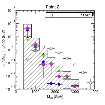
Figure 2: Signal and SM backgrounds for Point 2. See Fig. 1 for symbols.

Figure 3: Signal and SM backgrounds for Point 3. See Fig. 1 for symbols.

Figure 4: Signal and SM backgrounds for Point 4. See Fig. 1 for symbols.

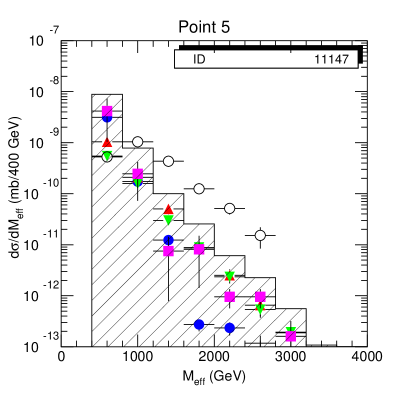
Figure 5: Signal and SM backgrounds for Point 5. See Fig. 1 for symbols.

2 Effective Mass Analysis

The first step after discovering a deviation from the SM is to estimate the mass scale. SUSY production at the LHC is dominated by gluinos and squarks, which decay into jets plus missing energy. The mass scale can be estimated using the effective mass, defined as the scalar sum of the $p_{T}$’s of the four hardest jets and the missing transverse energy $\hbox to0.0pt{\hbox to7.95831pt{\hfil/\hfil}\hss}E_{T}$,

$$M_{\rm eff}=p_{T,1}+p_{T,2}+p_{T,3}+p_{T,4}+\hbox to0.0pt{\hbox to7.95831pt{\hfil/\hfil}\hss}E_{T}\,.$$

ISAJET 7.20 [5] was used to generate samples of 10K events for each signal point, 50K events for each of $t\bar{t}$, $Wj$ with $W\to e\nu,\mu\nu,\tau\nu$, and $Zj$ with $Z\to\nu\bar{\nu},\tau\tau$ in five bins covering $50<p_{T}<1600\,{\rm GeV}$, and 2500K QCD events, i.e., primary $g$, $u$, $d$, $s$, $c$, or $b$ jets, in five bins covering $50<p_{T}<2400\,{\rm GeV}$. The detector response was simulated using a toy calorimeter with

$${\rm EMCAL} 10\%/\sqrt{E}+1\%$$

$${\rm HCAL} 50\%/\sqrt{E}+3\%$$

$${\rm FCAL} 100\%/\sqrt{E}+7\%,\ |\eta|>3\,.$$

Jets were found using a simple fixed-cone algorithm (GETJET) with $R=[(\Delta\eta)^{2}+(\Delta\phi)^{2}]^{1/2}=0.7$. To suppress the SM background, the following cuts were made:

• $\hbox to0.0pt{\hbox to7.95831pt{\hfil/\hfil}\hss}E_{T}>100\,{\rm GeV}$

• $\geq 4$ jets with $p_{T}>50\,{\rm GeV}$ and $p_{T,1}>100\,{\rm GeV}$

• Transverse sphericity $S_{T}>0.2$

• Lepton veto

• $\hbox to0.0pt{\hbox to7.95831pt{\hfil/\hfil}\hss}E_{T}>0.2M_{\rm eff}$

With these cuts and the idealized detector assumed here, the signal is much larger than the SM backgrounds for large $M_{\rm eff}$, as is illustrated in Figs. 1–5.

Table 2: The value of $M_{\rm eff}$ for which $S=B$ compared to $M_{\rm SUSY}$, the lighter of the gluino and squark masses. Note that Point 4 is strongly influenced by the $\hbox to0.0pt{\hbox to7.95831pt{\hfil/\hfil}\hss}E_{T}$ and jet $p_{T}$ cuts.

Point	$M_{\rm eff}\,({\rm GeV})$	$M_{\rm SUSY}\,({\rm GeV})$	Ratio
1	0980	663	1.48
2	1360	926	1.47
3	1420	928	1.53
4	0470	300	1.58
5	0980	586	1.67

The peak of the $M_{\rm eff}$ mass distribution, or alternatively the point at which the signal and background are equal, provides a good first estimate of the SUSY mass scale, which is defined to be

$$M_{\rm SUSY}=\min(M_{\tilde{g}},M_{\tilde{u}_{R}})$$

(The choice of $M_{\tilde{u}_{R}}$ as the typical squark mass is arbitrary.) The ratio of the value $M_{\rm eff}$ for which $S=B$ to $M_{\rm SUSY}$ was calculated by fitting smooth curves to the signal and background and is given in Table II. To see whether the approximate constancy of this ratio might be an accident, 100 SUGRA models were chosen at random with $100<m_{0}<500\,{\rm GeV}$, $100<m_{1/2}<500\,{\rm GeV}$, $-500<A_{0}<500\,{\rm GeV}$, $1.8<\tan\beta<12$, and $\mathop{\rm sgn}\mu=\pm 1$ and compared to the assumed signal, Point 1. The light Higgs was assumed to be known, and all the comparison models were required to have $M_{h}=100.4\pm 3\,{\rm GeV}$. A sample of 1K events was generated for each point, and the peak of the $M_{\rm eff}$ distribution was found by fitting a Gaussian near the peak. Figure 6 shows the resulting scatter plot of $M_{\rm SUSY}$ vs. $M_{\rm eff}$. The ratio is constant within about $\pm 10\%$, as can be seen from Fig. 7. This error is conservative, since there considerable contribution to the scatter from the limited statistics and the rather crude manner in which the peak was found.

Figure 6: Scatter plot of $M_{\rm SUSY}=\min(M_{\tilde{g}},M_{\tilde{u}})$ vs. $M_{\rm eff}$ for randomly chosen SUGRA models having the same light Higgs mass within $\pm 3\,{\rm GeV}$ as Point 1.

Figure 7: Ratio $M_{\rm eff}/M_{\rm SUSY}$ from Fig. 6

3 Selection of $h\rightarrow b\bar{b}$

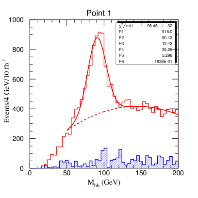
Figure 8: $M(b\bar{b})$ for pairs of $b$ jets for the Point 1 signal (open histogram) and for the sum of all backgrounds (shaded histogram) after cuts described in the text. The smooth curve is a Gaussian plus quadratic fit to the signal. The light Higgs mass is $100.4\,{\rm GeV}$.

For Point 1 the decay chain $\tilde{\chi}_{2}^{0}\rightarrow\tilde{\chi}_{1}^{0}h$, $h\rightarrow b\bar{b}$ has a large branching ratio, as is typical if this decay is kinematically allowed. The decay $h\rightarrow b\bar{b}$ thus provides a handle for identifying events containing $\tilde{\chi}_{2}^{0}$’s [6]. Furthermore, the gluino is heavier than the squarks and so decays into them. The strategy for this analysis is to select events in which one squark decays via

$$\tilde{q}\rightarrow\tilde{\chi}_{2}^{0}q,\ \tilde{\chi}_{2}^{0}\rightarrow\tilde{\chi}_{1}^{0}h,\ h\rightarrow b\bar{b}\,,$$

and the other via

$$\tilde{q}\rightarrow\tilde{\chi}_{1}^{0}q\,,$$

giving two $b$ jets and exactly two additional hard jets.

ISAJET 7.22 [5] was used to generate a sample of 100K events for Point 1, corresponding to about $5.6\,{\rm fb}^{-1}$. Background samples of 250K each for $t\bar{t}$, $Wj$, and $Zj$, and 5000K for QCD jets were also generated, equally divided among five $p_{T}$ bins. The background samples generally represent a small fraction of an LHC year. The detector response was simulated using the toy calorimeter described above. Jets were found using a fixed cone algorithm with $R=0.4$. The following cuts were imposed:

• $\hbox to0.0pt{\hbox to7.95831pt{\hfil/\hfil}\hss}E_{T}>100\,{\rm GeV}$

• $\geq 4$ jets with $p_{T}>50\,{\rm GeV}$ and $p_{T,1}>100\,{\rm GeV}$

• Transverse sphericity $S_{T}>0.2$

• $M_{\rm eff}>800\,{\rm GeV}$

• $\hbox to0.0pt{\hbox to7.95831pt{\hfil/\hfil}\hss}E_{T}>0.2M_{\rm eff}$

Jets were tagged as $b$’s if they contained a $B$ hadron with $p_{T}>5\,{\rm GeV}$ and $\eta<2$; no other tagging inefficiency or $b$ mistagging was included. Figure 8 shows the resulting $b\bar{b}$ mass distributions for the signal and the sum of all SM backgrounds with $p_{T,b}>25\,{\rm GeV}$ together with a Gaussian plus quadratic fit to the signal. At a luminosity of $10^{33}\,{\rm cm}^{-2}{\rm s}^{-1}$, ATLAS will have a $b$-jet tagging efficiency of 70% for a rejection of 100 [1]. Hence, the number of events should be reduced by a factor of about two, but the mistagging background is probably small compared to the real background shown. The Higgs mass peak is shifted downward somewhat; using a larger cone, $R=0.7$, gives a peak which is closer to the true mass but wider.

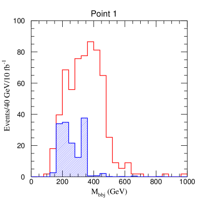
Figure 9: The smaller of the two $b\bar{b}j$ masses for signal and background events with $73<M(b\bar{b})<111\,{\rm GeV}$ in Fig. 8 and with exactly two additional jets $j$ with $p_{T}>75\,{\rm GeV}$. The endpoint of this distribution should be approximately the mass difference between the squark and the $\tilde{\chi}_{1}^{0}$, about $542\,{\rm GeV}$.

Events were then required to have exactly one $b\bar{b}$ pair with $73<M(b\bar{b})<111\,{\rm GeV}$ and exactly two additional jets with $p_{T}>75\,{\rm GeV}$. The invariant mass of each jet with the $b\bar{b}$ pair was calculated. For the desired decay chain, one of these two must come from the decay of a single squark, so the smaller of them must be less than the kinematic limit for single squark decay, $M(\tilde{u}_{R})-M(\tilde{\chi}_{1}^{0})=542\,{\rm GeV}$. The smaller of the two $b\bar{b}j$ masses is plotted in Fig. 9 for the signal and for the sum of all backgrounds and shows the expected edge. The SM background shows fluctuations from the limited Monte Carlo statistics but seems to be small near the edge, at least for the idealized detector considered here. There is some background from the SUSY events above the edge, presumably from other decay modes and/or initial state radiation.

4 Selection of $W\rightarrow q\bar{q}$

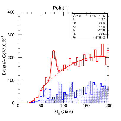
Figure 10: $M_{34}$ for non-$b$ jets in events with two $200\,{\rm GeV}$ jets and two $50\,{\rm GeV}$ jets for the Point 1 signal (open histogram) and the sum of all backgrounds (shaded histogram).

Point 1 also has a large combined branching ratio for one gluino to decay via

$$\tilde{g}\rightarrow\tilde{q}_{L}\bar{q},\ \tilde{q}_{L}\rightarrow\tilde{\chi}_{1}^{\pm}q,\ \tilde{\chi}_{1}^{\pm}\rightarrow\tilde{\chi}_{1}^{0}W^{\pm},\ W^{\pm}\rightarrow q\bar{q}\,,$$

and the other via

$$\tilde{g}\rightarrow\tilde{q}_{R}q,\ \tilde{q}_{R}\rightarrow\tilde{\chi}_{1}^{0}q\,,$$

giving two hard jets and two softer jets from the $W$. The branching ratio for $\tilde{q}_{L}\rightarrow\tilde{\chi}_{1}^{0}q$ is small for Point 1, so the contributions from $\tilde{g}\rightarrow\tilde{q}_{L}\bar{q}$ and from $\tilde{q}_{L}\tilde{q}_{L}$ pair production are suppressed.

The same signal sample was used as in Section III, and jets were again found using a fixed cone algorithm with $R=0.4$. The combinatorial background for this decay chain is much larger than for the previous one, so harder cuts are needed:

• $\hbox to0.0pt{\hbox to7.95831pt{\hfil/\hfil}\hss}E_{T}>100\,{\rm GeV}$

• $\geq 4$ jets with $p_{T1,2}>200\,{\rm GeV}$, $p_{T3,4}>50\,{\rm GeV}$, and $\eta_{3,4}<2$

• Transverse sphericity $S_{T}>0.2$

• $M_{\rm eff}>800\,{\rm GeV}$

• $\hbox to0.0pt{\hbox to7.95831pt{\hfil/\hfil}\hss}E_{T}>0.2M_{\rm eff}$

The same $b$-tagging algorithm was applied to tag the third and fourth jets as not being $b$ jets. Of course, this is not really feasible; instead one should measure the $b$-jet distributions and subtract them.

The mass distribution $M_{34}$ of the third and fourth highest $p_{T}$ jets with these cuts is shown in Fig. 10 for the signal and the sum of all backgrounds. A peak is seen a bit below the $W$ mass with a fitted width surprisingly smaller than that for the $h$ in Fig. 8, note that the $W$ natural width has been neglected in the simulation of the decays. The SM background is more significant here than for $h\to b\bar{b}$. Events from this peak can be combined with another jet as was done for $h\rightarrow b\bar{b}$ in Fig. 9, providing another determination of the squark mass. Figure 10 also provides a starting point for measuring $W$ decays separately from other sources of leptons such as gaugino decays into sleptons.

5 Selection of $\tilde{\chi}_{2}^{0}\rightarrow\tilde{\ell}\ell\rightarrow\tilde{\chi}_{1}^{0}\ell\ell$

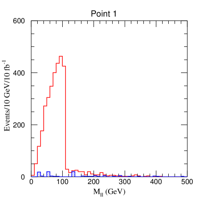
Figure 11: $M_{\ell\ell}$ for the Point 1 signal (open histogram) and the sum of all backgrounds (shaded histogram).

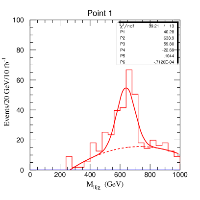
Figure 12: $M_{\ell\ell j\tilde{\chi}_{1}^{0}}$ for events with $86<M_{\ell\ell}<109\,{\rm GeV}$ in Fig. 11, using $\vec{p}_{\tilde{\chi}_{1}^{0}}=M_{\tilde{\chi}_{1}^{0}}/M_{\ell\ell}\vec{p}_{\ell\ell}$ for the Point 1 signal (open histogram) and the SM background (shaded histogram).

Point 1 has relatively light sleptons, which is generically necessary if the $\tilde{\chi}_{1}^{0}$ is to provide acceptable cold dark matter [7]. Hence the two-body decay

$$\tilde{\chi}_{2}^{0}\rightarrow\tilde{\ell}_{R}\ell\rightarrow\tilde{\chi}_{1}^{0}\ell^{+}\ell^{-}$$

is kinematically allowed and competes with the $\tilde{\chi}_{2}^{0}\rightarrow\tilde{\chi}_{1}^{0}h$ decay, producing opposite-sign, like-flavor dileptons. The largest SM background is $t\bar{t}$. To suppress this and other SM backgrounds the following cuts were made on the same signal and SM background samples used in the two previous sections:

• $M_{\rm eff}>800\,{\rm GeV}$

• $\hbox to0.0pt{\hbox to7.95831pt{\hfil/\hfil}\hss}E_{T}>0.2M_{\rm eff}$

• $\geq 1$ $R=0.4$ jet with $p_{T,1}>100\,{\rm GeV}$

• $\ell^{+}\ell^{-}$ pair with $p_{T,\ell}>10\,{\rm GeV}$, $\eta_{\ell}<2.5$

• $\ell$ isolation cut: $E_{T}<10\,{\rm GeV}$ in $R=0.2$

• Transverse sphericity $S_{T}>0.2$

With these cuts very little SM background survives, and the $M_{\ell\ell}$ mass distribution shown in Fig. 11 has an edge near

$$M_{\ell\ell}^{\rm max}=M_{\tilde{\chi}_{2}^{0}}\sqrt{1-{M_{\tilde{\ell}}^{2}\over M_{\tilde{\chi}_{2}^{0}}^{2}}}\sqrt{1-{M_{\tilde{\chi}_{1}^{0}}^{2}\over M_{\tilde{\ell}}^{2}}}\approx 112\,{\rm GeV}\,,$$

If $M_{\ell\ell}$ is near its kinematic limit, then the velocity difference of the $\ell^{+}\ell^{-}$ pair and the $\tilde{\chi}_{1}^{0}$ is minimized. Having both leptons hard requires $M_{\tilde{\ell}}/M_{\tilde{\chi}_{2}^{0}}^{2}\sim M_{\tilde{\chi}_{1}^{0}}/M_{\tilde{\ell}}$. Assuming this and $M_{\tilde{\chi}_{2}^{0}}=2M_{\tilde{\chi}_{1}^{0}}$ implies that the endpoint in Fig. 11 is equal to the $\tilde{\chi}_{1}^{0}$ mass. An improved estimate could be made by detailed fitting of all the kinematic distributions. Events were selected with $M_{\ell\ell}^{\rm max}-10\,{\rm GeV}<M_{\ell\ell}<M_{\ell\ell}^{\rm max}$, and the $\tilde{\chi}_{1}^{0}$ momentum was calculated using this crude $\tilde{\chi}_{1}^{0}$ mass and

$$\vec{p}_{\tilde{\chi}_{1}^{0}}=(M_{\tilde{\chi}_{1}^{0}}/M_{\ell\ell})\,\vec{p}_{\ell\ell}\,.$$

The invariant mass $M_{\ell\ell j\tilde{\chi}_{1}^{0}}$ of the $\ell^{+}\ell^{-}$, the highest $p_{T}$ jet, and the $\tilde{\chi}_{1}^{0}$ was then calculated and is shown in Fig. 12. A peak is seen near the light squark masses, 660–$688\,{\rm GeV}$. More study is needed, but this approach looks promising.

This work would have been impossible without the contributions of my collaborators on ISAJET, H. Baer, S. Protopopescu, and X. Tata. It was supported in part by the United States Department of Energy under contract DE-AC02-76CH00016.

References

- [1] ATLAS Collaboration, Technical Proposal, LHCC/P2 (1994).
- [2] CMS Collaboration, Technical Proposal, LHCC/P1 (1994).
- [3] H. Baer, C.-H. Chen, F. Paige, and X. Tata, Phys. Rev. D52, 2746 (1995); Phys. Rev. D53, 6241 (1996).
- [4] A. Bartl, J. Soderqvist, et al., these proceedings.
- [5] F. Paige and S. Protopopescu, in Supercollider Physics, p. 41, ed. D. Soper (World Scientific, 1986); H. Baer, F. Paige, S. Protopopescu and X. Tata, in Proceedings of the Workshop on Physics at Current Accelerators and Supercolliders, ed. J. Hewett, A. White and D. Zeppenfeld, (Argonne National Laboratory, 1993).
- [6] D. Froidevaux and E. Richter-Was, presentation to ATLAS Collaboration Meeting (June, 1996).
- [7] H. Baer and M. Brhlik, Phys. Rev. D53, 597 (1996).