The structure functions and parton momenta distribution in the hadron rest system

Abstract

The alternative to the standard formulation of QPM in the infinite momentum frame is suggested. The proposed approach does not require any extra assumptions in addition, consistently takes into account the parton transversal momenta and does not prefer any special reference system. The standard approach is involved as a limiting case. In the result the modified relations between the structure and distribution functions are obtained together with some constraint on their shape. The comparison with experimental data offers a speculation about values of effective masses of quarks, which emerge as a free parameter in the approach.

1 Introduction

The deep inelastic scattering (DIS) of leptons on the nucleons and nuclei has been since early seventies the powerful tool for investigation of the nucleon internal structure and simultaneously has served as an crucial test of the related theory - QCD. For recent results in this field see e.g. [1] and citations therein.

The quark-parton model (QPM), motivated by the experimental data, is extraordinarily simple if formulated in the reference system in which the nucleon is fast moving (infinite momentum frame - IMF). Namely in this system the Bjorken scaling variable $x_{B}$ can be approximately identified with the momentum fraction of the nucleon carried by a parton and experimentally measured structure functions can be easily related to the combinations of distribution functions expressed in terms of $x_{B}$. The distribution functions extracted from the experimental data by the global analysis (see e.g. [13]) relying on QPM+QCD represent basic elements of the present picture of nucleons and other hadrons.

In this paper we attempt to cope with the not only aesthetic drawback of QPM which in the standard formulation has a good sense only in the preferred reference system - IMF. The idea of alternatives to the QPM postulated in IMF is not new, the possibility to obtain in some approximation the structure and distribution functions from a definite parton model formulated in the nucleon rest frame has been shown e.g. in [2],[3],[5] and recently [4],[6]. We suggest rather a consistent modification of the general standard formulation which does not adhere necessarily to IMF and simultaneously does not require any special assumptions in addition. The basis of our considerations are only kinematics and mathematics.

The paper is organized as follows. In the following section the basic kinematic quantities related to the DIS are introduced and particularly the meaning of variable $x_{B}$ is discussed. In the Sec.3 we formally apply the standard assumptions of the QPM to the nucleon in its rest system (LAB) and compare the results with those normally related to the IMF. The Sec.4 is devoted to the discussion from more physical point of view together with the glance at experimental data on proton structure function $F_{2}$. The last section shortly summarizes the possible conclusions.

2 Kinematics

First of all let us recall some basic notions used in the description of DIS and the interpretation of the experimental data on the basis of QPM. The process is usually described (see Fig.1) by the variables

$$q^{2}\equiv-Q^{2}=(k-k^{\prime})^{2},\qquad x_{B}=\frac{Q^{2}}{2Pq}$$ (2.1)

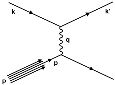
Figure 1: Diagram describing DIS as a one photon exchange between the charged lepton and parton.

As a rule, lepton mass is neglected, i.e. $k^{2}=k^{\prime 2}=0$. Important assumption of QPM is that struck parton remains on-shell, that implies

$$q^{2}+2pq=0$$ (2.2)

Bjorken scaling variable $x_{B}$ can be interpreted as the fraction of the nucleon momentum carried by the parton in the nucleon infinite momentum frame (IMF). The motivation of this statement can be explained as follows. Let us denote

$$p(lab)\equiv(p_{0},p_{1},p_{2},p_{3}),\qquad P(lab)\equiv(M,0,0,0),\qquad q(lab)\equiv(q_{0},q_{1},q_{2},q_{3})$$ (2.3)

fourmometa of the parton, nucleon and exchanged photon in the nucleon rest system (LAB). The Lorentz boost to the IMF (in the direction of collision axis) gives

$$p(\inf)\equiv(p_{0}^{\prime},p_{1}^{\prime},p_{2},p_{3}),\qquad P(\inf)\equiv(P_{0}^{\prime},P_{1}^{\prime},0,0),\qquad q(\inf)\equiv(q_{0}^{\prime},q_{1}^{\prime},q_{2},q_{3})$$ (2.4)

where for $\beta\rightarrow-1$

$$p_{0}^{\prime}=p_{1}^{\prime}=\gamma(p_{0}+p_{1}),\quad P_{0}^{\prime}=P_{1}^{\prime}=\gamma M,\qquad\gamma=1/\sqrt{1-\beta^{2}}$$ (2.5)

If we denote

$$x\equiv\frac{p_{0}^{\prime}}{P_{0}^{\prime}}=\frac{p_{1}^{\prime}}{P_{1}^{\prime}}=\frac{p_{0}+p_{1}}{M}$$ (2.6)

then one can write

$$p(\inf)=xP(\inf)+(0,0,p_{2},p_{3})$$ (2.7)

Now let the lepton has initial momentum $k(lab)\equiv(k_{0},-k_{0},0,0)$. If we denote $\nu\equiv k_{0}-k_{0}^{\prime}$ and $q_{L}\equiv q_{1},$ then $q_{L}<0$ and from Eqs. (2.1), (2.2) it follows

$$x_{B}=\frac{pq}{Pq}=\frac{p_{0}\nu+\mid q_{L}\mid p_{1}}{M\nu}-\frac{\overrightarrow{p_{T}}\overrightarrow{q_{T}}}{M\nu}$$ (2.8)

where $\overrightarrow{p_{T}},\ \,\overrightarrow{q_{T}}$ are the parton and photon transversal momenta . Obviously

$$k^{\prime 2}=(k-q)^{2}=k^{2}+q^{2}-2k_{0}\nu+2k_{0}\mid q_{L}\mid=0$$

$$\frac{\mid q_{L}\mid}{\nu}=1+\frac{Q^{2}}{2k_{0}\nu}=1+\frac{M}{k_{0}}x_{B}$$ (2.9)

Using this relation the Eq.(2.8) can be modified

$$x_{B}=\frac{p_{0}+p_{1}}{M}+\frac{p_{1}}{k_{0}}x_{B}-\frac{\overrightarrow{p_{T}}\overrightarrow{q_{T}}}{M\nu}$$ (2.10)

therefore if the lepton energy is sufficiently high, so $p_{1}/k_{0}\approx 0$, one can write

$$x_{B}=x-\frac{p_{T}\ \,q_{T}}{M\nu}\cos\varphi$$ (2.11)

where $\varphi$ is the angle between the parton and photon momenta in the transversal plane.

So, if parton transversal momenta are neglected, $x_{B}$ really represents fraction of momentum (2.6). In a higher approximation the experimentally measured $x_{B}$ being an integral over $\varphi$ is effectively smeared with respect to the fraction $x-$ which is not correlated with $\varphi.$ An estimation of the second term in the last equation can be done as follows. Because

$$q^{2}=\nu^{2}-\left|\overrightarrow{q}\right|^{2}$$

$$\left(\frac{\overrightarrow{q}}{\nu}\right)^{2}=1+\frac{Q^{2}}{\nu^{2}}=1+\frac{4M^{2}}{Q^{2}}x_{B}^{2}$$ (2.12)

then (2.9), (2.12) give

$$\frac{q_{T}}{\nu}=\sqrt{\left(\frac{\overrightarrow{q}}{\nu}\right)^{2}-\left(\frac{q_{L}}{\nu}\right)^{2}}=\sqrt{\left(\frac{4M^{2}}{Q^{2}}-\frac{M^{2}}{k_{0}^{2}}\right)x_{B}^{2}-\frac{2M}{k_{0}}x_{B}}<\frac{2Mx_{B}}{\sqrt{Q^{2}}}$$ (2.13)

therefore for $M/k_{0}\approx 0$ we obtain

$$\frac{pq}{M\nu}=\frac{p_{0}+p_{1}}{M}-\frac{2p_{T}x_{B}}{\sqrt{Q^{2}}}\cos\varphi$$ (2.14)

and

$$x_{B}=x-\frac{2p_{T}x_{B}}{\sqrt{Q^{2}}}\cos\varphi$$ (2.15)

Therefore $x_{B}$ can be at sufficiently high $Q^{2}$ considered as a good approximation of $x$ (and vice versa), on the end of next section we shall suggest how to treat this correction more accurately.

Let us note, the parameter $x$ (2.6) can be expressed also as

$$x\equiv\frac{p_{0}+p_{1}}{P_{0}+P_{1}}$$ (2.16)

and identified with light cone variable, which can be expressed also in terms of rapidity and transversal mass

$$x\equiv\frac{m_{T}}{M}\exp(y-y_{0}),\qquad m_{T}\equiv\sqrt{p_{T}^{2}+m^{2}},\qquad y\equiv\frac{1}{2}\ln\ \frac{p_{0}+p_{1}}{p_{0}-p_{1}}$$ (2.17)

where $y_{0}$ denotes the proton rapidity. In this form the parameter $x$ is invariant with respect to any Lorentz boost along the collision axis.

Now, if we assume parton phase space is spherical (in LAB) and rather idealized scenario in which the parton has a mass $m^{2}=p_{0}^{2}-p_{1}^{2}-p_{2}^{2}-p_{3}^{2}$, then further relations can be obtained.

1) variable x

From Eq.(2.6) and the condition $x\leq 1$ it can be shown

$$x\geq\frac{m^{2}}{M^{2}}$$ (2.18)

$$\sqrt{p_{1}^{2}+p_{2}^{2}+p_{3}^{2}}\leq p_{m}\equiv\frac{M^{2}-m^{2}}{2M},\qquad p_{T}^{2}\leq M^{2}(x-\frac{m^{2}}{M^{2}})(1-x)$$ (2.19)

Obviously, the highest value of $p_{1}$ is reached if $p_{T}=0$ and

$$x=\frac{\sqrt{p_{1}^{2}+m^{2}}+p_{1}}{M}=1$$ (2.20)

which gives

$$p_{1\max}=p_{m}\equiv\frac{M^{2}-m^{2}}{2M}$$ (2.21)

Then spherical symmetry implies

$$\sqrt{p_{1}^{2}+p_{2}^{2}+p_{3}^{2}}\leq p_{m}$$ (2.22)

i.e. the first relation in (2.19) is proved. Apparently, the minimal value of $x$ is reached for $p_{1}=-p_{m}$ and $p_{T}=0$. After inserting to (2.6) one gets (2.18). Finally, the relation (2.6) implies

$$p_{1}=\frac{M^{2}x^{2}-m^{2}-p_{T}^{2}}{2Mx}$$ (2.23)

which inserted to modified relation (2.22)

$$p_{1}^{2}+p_{T}^{2}\leq\left(\frac{M^{2}-m^{2}}{2M}\right)^{2}$$ (2.24)

after some computation gives the second relation in (2.19).

2) variable $x_{B}$

Let us express $x_{B}$ in the LAB

$$x_{B}=\frac{pq}{Pq}=\frac{p_{0}\nu-\overrightarrow{p}\ \overrightarrow{q}}{M\nu}=\frac{1}{M}\left(\sqrt{m^{2}+\left|\overrightarrow{p}\right|^{2}}-\frac{\overrightarrow{p}\ \overrightarrow{q}}{\nu}\right)$$ (2.25)

and estimate its minimal value. With the use of (2.12) we obtain

$$x_{B}\geq\frac{1}{M}\left(\sqrt{m^{2}+p_{m}^{2}}-p_{m}\sqrt{1+\frac{4M^{2}}{Q^{2}}x_{B}^{2}}\right)$$ (2.26)

Since

$$\sqrt{1+\frac{4M^{2}}{Q^{2}}x_{B}^{2}}\leq 1+\frac{2M^{2}}{Q^{2}}x_{B}^{2}$$ (2.27)

and

$$\frac{1}{M}\left(\sqrt{m^{2}+p_{m}^{2}}-p_{m}\right)=\frac{m^{2}}{M^{2}}$$ (2.28)

relation (2.26) can be rewritten

$$x_{B}\geq\frac{m^{2}}{M^{2}}-\frac{2Mp_{m}}{Q^{2}}x_{B}^{2}\geq\frac{m^{2}}{M^{2}}-\frac{2Mp_{m}}{Q^{2}}\frac{m^{4}}{M^{4}}=\frac{m^{2}}{M^{2}}(1-\frac{2p_{m}}{M}\frac{m^{2}}{Q^{2}})$$ (2.29)

i.e. for $m^{2}\ll Q^{2}$ lower limit of $x_{B}$ coincides with the limit (2.18).

3 Distribution of partons in the nucleon rest system

In this section we imagine partons as a gas (or a mixture of gases) of quasi free particles filling up the nucleon volume. The prefix quasi means that partons bounded inside the nucleon behave at the interaction with external photon probing the nucleon as free particles having the fourmomenta on mass shell. This is standard assumption of QPM, but whereas in the IMF parton masses are ”hidden”, in the description related to the LAB the masses will be present.

In the next section we shall discuss in which extent the results obtained for this idealized picture could be applied for more realistic scenario.

3.1 Deconvolution of the distribution function

Let us suppose $F(x)$ is the distribution function of some sort of partons given in terms of variable $x$ ($\ref{k6})$ and these partons are assumed to have the mass $m$. If the spherical symmetry is assumed in the hadron rest system and $G(p_{0})d^{3}p$ is the number of partons in the element of the phase space, then the distribution function $F(x)$ can be expressed as the convolution

$$F(x)=\int\delta\left(\frac{p_{0}+p_{1}}{M}-x\right)G(p_{0})d^{3}p,\qquad p_{0}=\sqrt{m^{2}+p_{1}^{2}+p_{2}^{2}+p_{3}^{2}}$$ (3.1)

Using the set of integral variables $h,p_{0},\varphi$ instead of $p_{1},p_{2},p_{3}$

$$p_{1}=h,\qquad p_{2}=\sqrt{p_{0}^{2}-m^{2}-h^{2}}\sin\varphi,\qquad p_{3}=\sqrt{p_{0}^{2}-m^{2}-h^{2}}\cos\varphi$$ (3.2)

the integral (3.1) can rewritten

$$F(x)=2\pi\int_{m}^{E_{\max}}\int_{-H}^{+H}\delta\left(\frac{p_{0}+h}{M}-x\right)G(p_{0})p_{0}dhdp_{0},\qquad H=\sqrt{p_{0}^{2}-m^{2}}$$ (3.3)

First of all we calculate inner integral within limits $\pm H$ depending on $p_{0}.$ For given $x$ and $p_{0}$ there contributes only $h$ for which

$$p_{0}+h=Mx$$ (3.4)

but simultaneously $h$ must be inside the limits

$$-\sqrt{p_{0}^{2}-m^{2}}\leq h\leq\sqrt{p_{0}^{2}-m^{2}}$$ (3.5)

which means, that for

$$p_{0}+\sqrt{p_{0}^{2}-m^{2}}<Mx$$ (3.6)

or equivalently for

$$p_{0}<\xi\equiv\frac{Mx}{2}+\frac{m^{2}}{2Mx}$$ (3.7)

considered integral gives zero. For $p_{0}>\xi$, when the both conditions (3.4), (3.5) are compatible for some value $h$ the integral can be evaluated

$$\int_{-H}^{+H}\delta\left(\frac{p_{0}+h}{M}-x\right)G(p_{0})p_{0}dh=MG(p_{0})p_{0}$$ (3.8)

Therefore the integral (3.3) can be expressed

$$F(x)=2\pi M\int_{\xi}^{E_{\max}}G(p_{0})p_{0}dp_{0}$$ (3.9)

Let us note, the equation similar to this appears already in [2] but with the structure function $F_{2}(x)$ instead of the distribution one. We shall deal with the $F_{2}$ in the next subsection, where it will be shown, that the corresponding equation is more complicated. For a comparison see also [5], where on the place of $G(p_{0})$ the statistical distribution characterized by some temperature and chemical potential is used.

Next, from the relation (3.7) we can express $x$ as a function $\xi$

$$x_{\pm}=\frac{\xi\pm\sqrt{\xi^{2}-m^{2}}}{M}$$ (3.10)

Using the relations (2.18), (3.7) one can easily check

$$1\geq x_{+}\geq\frac{m}{M}\geq x_{-}\geq\frac{m^{2}}{M^{2}},\qquad E_{\max}=\frac{M^{2}+m^{2}}{2M}\geq\xi\geq m$$ (3.11)

First let us insert $x_{+}$ into (3.9)

$$F\left(\frac{\xi+\sqrt{\xi^{2}-m^{2}}}{M}\right)=2\pi M\int_{\xi}^{E_{\max}}G(p_{0})p_{0}dp_{0}$$ (3.12)

Differentiation in respect to $\xi$ gives

$$G(\xi)=-\frac{1}{2\pi M^{2}}F^{\prime}\left(\frac{\xi+\sqrt{\xi^{2}-m^{2}}}{M}\right)\left(\frac{1}{\xi}+\frac{1}{\sqrt{\xi^{2}-m^{2}}}\right)$$ (3.13)

Now we integrate the density $G(p_{0})$ over angular variables obtaining

$$P(p_{0})dp_{0}\equiv\int_{\Omega}G(p_{0})d^{3}p=4\pi G(p_{0})p_{0}\sqrt{p_{0}^{2}-m^{2}}dp_{0}$$ (3.14)

and after inserting into (3.13) we get

$$P(p_{0})dp_{0}=-2F^{\prime}\left(\frac{p_{0}+\sqrt{p_{0}^{2}-m^{2}}}{M}\right)\frac{p_{0}+\sqrt{p_{0}^{2}-m^{2}}}{M}\frac{dp_{0}}{M}$$ (3.15)

Second root $x_{-}$ gives very similar result

$$P(p_{0})dp_{0}=+2F^{\prime}\left(\frac{p_{0}-\sqrt{p_{0}^{2}-m^{2}}}{M}\right)\frac{p_{0}-\sqrt{p_{0}^{2}-m^{2}}}{M}\frac{dp_{0}}{M}$$ (3.16)

From the definition

$$x_{\pm}\equiv\frac{p_{0}\pm\sqrt{p_{0}^{2}-m^{2}}}{M}$$ (3.17)

the useful relations easily follow

$$x_{+}x_{-}=\frac{m^{2}}{M^{2}},\qquad x_{+}+x_{-}=\frac{2p_{0}}{M},\qquad x_{+}-x_{-}=\frac{2\sqrt{p_{0}^{2}-m^{2}}}{M}$$ (3.18)

$$\frac{dp_{0}}{M}=\frac{1}{2}(1-\frac{m^{2}}{M^{2}x_{\pm}^{2}})dx_{\pm},\qquad\frac{dx_{+}}{x_{+}}=-\frac{dx_{-}}{x_{-}}$$ (3.19)

Now, the equations (3.15), (3.16) can be joined

$$P(p_{0})=\mp\frac{2}{M}F^{\prime}(x_{\pm})x_{\pm}$$ (3.20)

How to understand the two different partial intervals (3.11) of $x$ give independently the complete distribution $P(p_{0})$ in Eq.(3.20)? It is due to the fact that e.g. $x_{-}$ represents in the integral (3.1) the region

$$\frac{\sqrt{p_{1}^{2}+p_{T}^{2}+m^{2}}+p_{1}}{M}=x_{-}\leq\frac{m}{M}$$ (3.21)

given by the paraboloid

$$p_{T}^{2}\leq 2m\left|p_{1}\right|,\qquad p_{1}\leq 0$$ (3.22)

containing complete information about $G(p_{0})$ which is spherically symmetric. The similar argument is valid for $x_{+}$ representing the rest of sphere. The Eqs.(3.15), (3.16) imply the similarity of $F(x)$ in both intervals

$$\frac{F^{\prime}(x_{+})x_{+}}{F^{\prime}(x_{-})x_{-}}=-1$$ (3.23)

which with the use of second relation (3.19) can be easily shown to be equivalent to

$$F(x_{+})=F(x_{-})$$ (3.24)

The relation (3.20) implies the distribution function $F(x)$ should be increasing for $(m/M)^{2}<x<m/M$ and decreasing for $m/M<x<1$ e.g. as shown in Fig.2. Now let us calculate the following integrals.

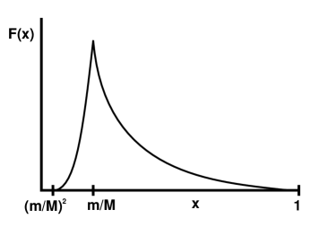
Figure 2: Example of the function obeying Eqs.(3.23), (3.24).

The total number $N$ of partons:

$$N=\int_{m}^{E_{\max}}P(p_{0})dp_{0}=-\int_{m/M}^{1}F^{\prime}(x_{+})(x_{+}-\frac{m^{2}}{M^{2}x_{+}})dx_{+}=$$

$$=-\int_{m/M}^{1}F^{\prime}(x_{+})x_{+}dx_{+}+\int_{m/M}^{1}F^{\prime}(x_{+})x_{-}dx_{+}$$ (3.25)

The last integral can be modified with the use of (3.19), (3.23)

$$\int_{m/M}^{1}F^{\prime}(x_{+})x_{-}dx_{+}=-\int_{m/M}^{1}F^{\prime}(x_{-})x_{-}^{2}\frac{dx_{+}}{x_{+}}=\int_{m/M}^{m^{2}/M^{2}}F^{\prime}(x_{-})x_{-}dx_{-}$$ (3.26)

Then integration by parts gives

$$N=-\int_{m^{2}/M^{2}}^{1}F^{\prime}(x)xdx=\int_{m^{2}/M^{2}}^{1}F(x)dx$$ (3.27)

The total energy $E$ of partons:

$$E=\int_{m}^{E_{\max}}P(p_{0})p_{0}dp_{0}=-\int_{m/M}^{1}F^{\prime}(x_{+})(x_{+}-\frac{m^{2}}{M^{2}x_{+}})\frac{M}{2}(x_{+}+x_{-})dx_{+}=$$

$$=-\frac{M}{2}\int_{m/M}^{1}F^{\prime}(x_{+})(x_{+}^{2}-x_{-}^{2})dx_{+}$$ (3.28)

A similar procedure as for $N$ then gives the result

$$E=-\frac{M}{2}\int_{m^{2}/M^{2}}^{1}F^{\prime}(x)x^{2}dx=M\int_{m^{2}/M^{2}}^{1}F(x)xdx$$ (3.29)

Therefore, the both descriptions based either on IMF variable $x$ or the parton energy $p_{0}$ in the LAB give the consistent results on the total number of partons and the fraction of energy carried by the partons.

3.2 The structure function

An important connection between the structure and distribution functions can be derived by a few (equivalent) ways, see e.g. textbooks [7],[8],[9]. In this paper we confine ourself to the electromagnetic unpolarized structure functions assuming spin 1/2. The general form of cross section for the scattering electron + proton and electron + point like, Dirac particle can be written

$$d\sigma(e^{-}+p)=\frac{e^{4}}{q^{4}}\frac{1}{4\sqrt{(kP)^{2}-m_{e}^{2}M^{2}}}K^{\alpha\beta}W_{\alpha\beta}4\pi M\frac{d^{3}k^{\prime}}{2k_{0}^{\prime}(2\pi)^{3}}$$ (3.30)

$$d\sigma(e^{-}+l)=\frac{e^{4}}{q^{4}}\frac{1}{4\sqrt{(kp)^{2}-m_{e}^{2}m_{l}^{2}}}K^{\alpha\beta}L_{\alpha\beta}2\pi\delta((p+q)^{2}-m^{2})\frac{d^{3}k^{\prime}}{2k_{0}^{\prime}(2\pi)^{3}}$$ (3.31)

where electron tensor has the standard form

$$K^{\alpha\beta}=2(k^{\alpha}k^{\prime\beta}+k^{\prime\alpha}k^{\beta}+g^{\alpha\beta}\frac{q^{2}}{2})$$ (3.32)

and the remaining hadron and lepton tensors $W_{\alpha\beta},$ $L_{\alpha\beta}$ can be written in the ”reduced” shape

$$W_{\alpha\beta}=\frac{P_{\alpha}P_{\beta}}{M^{2}}W_{2}-g_{\alpha\beta}W_{1}$$ (3.33)

$$L_{\alpha\beta}=4p_{\alpha}p_{\beta}-2g_{\alpha\beta}pq$$ (3.34)

General assumption that the scattering on proton is realized via scattering on the partons implies

$$d\sigma(e^{-}+p)=\int F(\xi)d\sigma(e^{-}+l)d\xi$$ (3.35)

where $F(\xi)$ is a function describing distribution of partons according to some parameter(s) $\xi.$ Now, if $F(\xi)$ is substituted by the usual distribution function and we assume

$$p_{\alpha}\approx\xi P_{\alpha}$$ (3.36)

then it is obvious, that Eq.(3.35) will be fulfilled provided that

$$P_{\alpha}P_{\beta}\frac{W_{2}}{M^{2}}-g_{\alpha\beta}W_{1}=\frac{1}{M}\int\frac{F(\xi)}{\xi}(2\xi^{2}P_{\alpha}P_{\beta}-g_{\alpha\beta}\,\xi Pq)\delta((\xi P+q)^{2}-m^{2})d\xi$$ (3.37)

For simplicity in this equation and anywhere in the next the weighting by the parton charges is omitted. In fact the Eq.(3.37) is just a master equation in [7](lesson 27, Eq.(27.4)), from which the known relations are derived

$$2MW_{1}(q^{2},\nu)=\frac{F_{2}(x)}{x},\qquad xF(x)=F_{2}(x)\equiv\nu W_{2}(q^{2},\nu),\qquad x\equiv\frac{-q^{2}}{2M\nu}$$ (3.38)

Here, let us point out, this result is based on the approximation (3.36), which is acceptable in IMF, but in addition only if parton transversal momenta are neglected. Actually, relation (3.36) would be exact only in the (unrealistic) case, when the partons are without any motion inside the nucleon, then the distribution function describes momenta fractions in any reference frame (including IMF), therefore describes also distribution of parton masses $\xi=m/M$.

Before repeating the above procedure for our distribution $G(p_{0})d^{3}p$ in LAB, one has correctly account for the flux factor corresponding to partons moving inside the proton volume. For $k\equiv(k_{0},-k_{0},0,0)$ the flux factor in (3.31)

$$4\sqrt{(kp)^{2}-m_{e}^{2}m_{l}^{2}}=4k_{0}(p_{0}+p_{1})=4k_{0}p_{0}(1+v_{1})$$ (3.39)

corresponds for some fixed $p$ to the subset of partons moving with velocity $\overrightarrow{v}=\overrightarrow{p}/p_{0}$. If this velocity has the opposite direction to the probing electron, then after passing through the whole subset $G(p_{0})d^{3}p$ the electron has not still reached backward boundary of the proton, where meanwhile the new partons appeared. And on contrary, if the velocity of subset has the same direction as the electron, then not all of these partons have the same chance to meet this electron. Namely, the partons close to the backward boundary are excluded from the game sooner than the electron reaches them. Quantitatively, the number of partons limited by the proton volume and having chance to meet the electron (with velocity $\sim 1)$ will be

$$dN=(1+v_{1})G(p_{0})d^{3}p$$ (3.40)

Including this correction to the flux factor (3.39), then instead of Eq.(3.37) we get the tensor equation

$$P_{\alpha}P_{\beta}\frac{W_{2}}{M^{2}}-g_{\alpha\beta}W_{1}+A(P_{\alpha}q_{\beta}+P_{\beta}q_{\alpha})+Bq_{\alpha}q_{\beta}=$$

$$=\frac{P_{0}}{M}\int\frac{G(p_{0})}{p_{0}}(2p_{\alpha}p_{\beta}-g_{\alpha\beta}\,pq)\delta((p+q)^{2}-m^{2})d^{3}p,\qquad p_{0}=\sqrt{m^{2}+p_{1}^{2}+p_{2}^{2}+p_{3}^{2}}$$ (3.41)

for which (3.36) is not required. The terms with the functions $A$ and $B$ do not contribute to the cross section (since $q_{\alpha}K^{\alpha\beta}=q_{\beta}K^{\alpha\beta}=0$), but generally must be included to ensure the equation consistence if the tensors are not gauge invariant. Also let us note, the correction similar to (3.40) was not used in the Eq.(3.37) since due to (3.36) the all partons in the applied approach have the same velocity as the proton.

Now the contracting of (3.41) with tensors $g^{\alpha\beta},q^{\alpha}q^{\beta},P^{\alpha}P^{\beta},P^{\alpha}q^{\beta}$ gives in the result set of four equations

$$W_{2}-4W_{1}+2M\nu(A-xB)=\frac{1}{M\nu}\int\frac{G(p_{0})}{p_{0}}[m^{2}-2Mx\nu]\delta\left(\frac{pq}{M\nu}-x\right)d^{3}p$$ (3.42)

$$\frac{\nu}{2Mx}W_{2}+W_{1}-2M\nu(A-xB)=\frac{1}{M\nu}\int\frac{G(p_{0})}{p_{0}}[Mx\nu]\delta\left(\frac{pq}{M\nu}-x\right)d^{3}p$$ (3.43)

$$W_{2}-W_{1}+\nu(2MA+\nu B)=\frac{1}{M\nu}\int\frac{G(p_{0})}{p_{0}}[p_{0}^{2}-\frac{Mx\nu}{2}]\delta\left(\frac{pq}{M\nu}-x\right)d^{3}p$$ (3.44)

$$W_{2}-W_{1}+(M\nu-2M^{2}x)A-2Mx\nu B=\frac{1}{M\nu}\int\frac{G(p_{0})}{p_{0}}[p_{0}Mx-\frac{Mx\nu}{2}]\delta\left(\frac{pq}{M\nu}-x\right)d^{3}p$$ (3.45)

in which the $\delta-$function from the integral (3.41) is expressed

$$\delta((p+q)^{2}-m^{2})=\delta(2pq+q^{2})=\delta\left(2M\nu\left(\frac{pq}{M\nu}-\frac{Q^{2}}{2M\nu}\right)\right)=\frac{1}{2M\nu}\delta\left(\frac{pq}{M\nu}-x\right)$$ (3.46)

If we define

$$V_{j}(x)\equiv\int G(p_{0})\left(\frac{p_{0}}{M}\right)^{j}\delta\left(\frac{pq}{M\nu}-x\right)d^{3}p,\qquad j=-1,0,1$$ (3.47)

then the solution of the set (3.42)-(3.45) reads

$$\begin{split}2MW_{1}&=\frac{\nu}{2Mx+\nu}\\ &\quad\cdot\left\{V_{-1}(x)\left[x-\frac{M}{\nu}\left(\frac{m^{2}}{M^{2}}-x^{2}\right)-2\frac{m^{2}x}{\nu^{2}}\right]+V_{0}(x)\frac{2Mx}{\nu}+V_{1}(x)\frac{2M^{2}x}{\nu^{2}}\right\}\end{split}$$ (3.48)

$$\begin{split}\nu W_{2}&=x\left(\frac{\nu}{2Mx+\nu}\right)^{2}\\ &\quad\cdot\left\{V_{-1}(x)\left[x-\frac{M}{\nu}\left(\frac{m^{2}}{M^{2}}+x^{2}\right)-2\frac{m^{2}x}{\nu^{2}}\right]+V_{0}(x)\frac{6Mx}{\nu}+V_{1}(x)\frac{6M^{2}x}{\nu^{2}}\right\}\end{split}$$ (3.49)

$$\begin{split}\nu^{2}MA&=-\left(\frac{\nu}{2Mx+\nu}\right)^{2}\\ &\quad\cdot\left\{V_{-1}(x)\left[\frac{1}{2}\left(\frac{m^{2}}{M^{2}}+3x^{2}\right)+\frac{m^{2}x}{M\nu}\right]-V_{0}(x)2x\left(1-\frac{Mx}{\nu}\right)-V_{1}(x)\frac{3Mx}{\nu}\right\}\end{split}$$ (3.50)

$$\begin{split}\nu^{3}B&=\left(\frac{\nu}{2Mx+\nu}\right)^{2}\\ &\quad\cdot\left\{V_{-1}(x)\left[\frac{1}{2}\left(\frac{m^{2}}{M^{2}}+3x^{2}\right)+\frac{m^{2}x}{M\nu}\right]-V_{0}(x)3x+V_{1}(x)\left(1-\frac{Mx}{\nu}\right)\right\}\end{split}$$ (3.51)

For next discussion we assume $\nu\gg M$, then

$$\nu W_{2}\equiv F_{2}(x)=x^{2}V_{-1}(x),\qquad MW_{1}\equiv F_{1}(x)=\frac{x}{2}V_{-1}(x)$$ (3.52)

so it is obvious the Callan-Gross relation $2xF_{1}=F_{2}$ holds in this approximation.

In the next step, following the Eq.(2.14), we accept the approximation

$$\frac{pq}{M\nu}\approx\frac{p_{0}+p_{1}}{M}$$ (3.53)

then the integrals (3.47) can be expressed

$$V_{j}(x)=\int G(p_{0})\left(\frac{p_{0}}{M}\right)^{j}\delta\left(\frac{p_{0}+p_{1}}{M}-x\right)d^{3}p,\qquad j=-1,0,1$$ (3.54)

This relation with the use of (3.1),(3.20) implies

$$\left(\frac{p_{0}}{M}\right)^{j}P(p_{0})=\mp\frac{2}{M}V_{j}^{\prime}(x_{\pm})x_{\pm},\qquad j=-1,0,1$$ (3.55)

where $x_{\pm}$ is defined in (3.17). The relations (3.55) and (3.18) give

$$\frac{V_{j}^{\prime}(x)}{V_{k}^{\prime}(x)}=\left(\frac{p_{0}}{M}\right)^{j-k}=\left(\frac{x_{+}+x_{-}}{2}\right)^{j-k}=\left(\frac{x}{2}+\frac{x_{0}^{2}}{2x}\right)^{j-k},\qquad x_{0}=\frac{m}{M}$$ (3.56)

In the previous section we have shown such functions as (3.54) obey the relation (3.24), which means in particular, that the functions have a maximum at $x_{0}$ and vanish for $x\leq x_{0}^{2}$. Therefore the same statement is valid also for functions $F_{2}/x^{2}$ and $F_{1}/x$ from Eq.(3.52)

$$\frac{F_{2}(x_{+})}{x_{+}^{2}}=\frac{F_{2}(x_{-})}{x_{-}^{2}},\qquad\frac{F_{1}(x_{+})}{x_{+}}=\frac{F_{1}(x_{-})}{x_{-}}$$ (3.57)

This means that the structure functions of our idealized hadron also have the maximum at $x_{0}$ or higher, if the peak of $V_{-1}(x)$ is not rather sharp. Obviously, the peak will be sharp if $P(p_{0})\neq 0$ for $p_{0}=m$. At the same time, it should be kept in mind, that due to (2.15) any function expressed in ”real” variable $x_{B}$ will be slightly smeared in view of this function expressed in $x$. That is just the case of the integrals (3.47) approximated by (3.54). But this smearing should be quite negligible for very low $x_{B}$ and high $Q^{2}$, see end of section 2.

Further, our considerations have started in previous section from the distribution function $F(x)$ for which we have obtained relation (3.20). The combination of this equation with (3.52), (3.55) and (3.18) gives

$$P(p_{0})=-\frac{1}{M}\left(\frac{F_{2}(x)}{x^{2}}\right)^{\prime}(x^{2}+x_{0}^{2}),\qquad x=\frac{p_{0}+\sqrt{p_{0}^{2}-m^{2}}}{M}$$ (3.58)

$$F^{\prime}(x)=\frac{1}{2}\left(\frac{F_{2}(x)}{x^{2}}\right)^{\prime}\left(x+\frac{x_{0}^{2}}{x}\right)$$ (3.59)

How to compare the last equation with the standard relation (3.38) for $F$ and $F_{2}$? As we have already told, the standard approach (3.37) is exact in the case when the partons are static with respect to the nucleon, i.e. when $x=m/M$. The Eq.(3.41) itself is more exact, but the further procedure with it requires the masses of the all partons in the considered subset being equal. Therefore for a comparison let us consider first the extreme scenario when the parton distribution functions $F(x)$ and $P(p_{0})$ are (see Eq.(3.20)) rather narrowly peaked around the points $x_{0}=m/M$ and $p_{0}=m$. Then for $x\approx x_{0}$ Eq.(3.59) gives

$$F^{\prime}(x)=\frac{1}{2}\left(\frac{F_{2}(x)}{x^{2}}\right)^{\prime}\left(x+\frac{x_{0}^{2}}{x}\right)\simeq\frac{1}{2}\frac{F_{2}^{\prime}(x)}{x_{0}^{2}}(x_{0}+x_{0})=\frac{F_{2}^{\prime}(x)}{x_{0}}$$ (3.60)

from which the second relation (3.38) follows as a limiting case of (3.59)

$$x_{0}F(x_{0})\approx F_{2}(x_{0})$$ (3.61)

Now, in the realistic case when the distribution functions are broad, the exact validity of (3.37) again requires static partons, therefore the corresponding distribution function represents also a spectrum of masses. But then obviously the above procedure for a single $m$ can be repeated with spectrum of masses $F(x_{0})$ giving in the result instead of (3.61) the relation

$$\int x_{0}F(x_{0})\delta(x-x_{0})dx_{0}=\int F_{2}(x_{0})\delta(x-x_{0})dx_{0}$$ (3.62)

which implies

$$xF(x)=F_{2}(x)$$ (3.63)

In this sense the approach based on Eq.(3.37) can be understood as a limiting case of that based on Eq.(3.41).

3.3 The high order corrections

The considerations of previous subsection are based on the approximation (3.53) which in the result gives relations (3.58), (3.59). Actually we had to calculate integrals (3.47) instead of (3.54) differing in the argument of $\delta$-function according to Eq.(2.14). The integrals (3.47) cannot be solved analytically according to the recipe for Eq.(3.1), however in principle their solution can by obtained by iterations. For example, first equation (3.52) reads

$$F_{2}(x)=x^{2}\int G(p_{0})\frac{M}{p_{0}}\delta\left(\frac{pq}{M\nu}-x\right)d^{3}p$$ (3.64)

Let us have some $F_{2}$, then algorithm of iterative procedure could be following:

0. step: $G_{0}$ is given by Eq.(3.58), $G$ is related to $P$ by (3.14).

1. step: Insert $G_{0}$ into (3.64), result of integration is some function $f_{1}(x).$ Make the difference $\Delta_{1}F_{2}=F_{2}-f_{1}$ and insert $\Delta_{1}F_{2}$ into (3.58), the relation gives the corresponding correction $\Delta_{1}G$. The result of this iterative step is $G_{1}=G_{0}+\Delta_{1}G.$ Then next steps will follow by analogy, on the end the corrected $G$ should be obtained.

More detailed discussion of considered correction exceeds scope of this paper and requires further study. The correction should be rather small, but let us remark that its evaluation requires some assumption about mass $m$ (or spectrum of masses). Also, let us note this correction together with terms $O(1/\nu)$ in (3.48),(3.49) introduces into the structure functions some $Q^{2}$ dependence having purely kinematic origin (we still assume $G$ being $Q^{2}$ independent). Obviously, all these corrections vanish for $Q^{2}\rightarrow\infty.$

4 Discussion

Are the considerations suggested in previous section compatible with the assumptions and philosophy of QPM and all that, is it legally to speak about distribution function in LAB? First, let us shortly recall standard interpretation of DIS in framework of QPM.

In the classical experiment, e.g. BCDMS [10] muons scatter on proton target at rest in the laboratory system. From measured angles and energies of the scattered muons one determines the invariant cross section as the function of kinematic invariants $x_{B},Q^{2}.$ Next, from this cross section the electromagnetic structure function $F_{2}(x_{B},Q^{2})$ is evaluated. The fact, that for sufficiently big $Q^{2}$ the structure function (approximately) scales $F_{2}(x_{B},Q^{2})\approx F_{2}(x_{B}),$ leads to the conclusion that in the experiment actually the scattering of two point-like particles takes place. This experimental fact is a basic motivation of the QPM in which it is postulated that the nucleon contains point-like electromagnetically active particles (partons), which can be for sufficiently high $Q^{2}$ treated as effectively free and their interaction with the muon is described by Feynman diagram with one photon exchange. That also means the struck partons remain on-mass shell. These assumptions should be fulfilled first of all in the system, where our experiment is done, i.e. in LAB. Of course, another point is, that in this system the picture of partons is in some respect obscured by the fact, that we do not know more about the kinematics of partons, their momenta, energies. The picture is quite clarified, when we change over from LAB to the IMF. Then the masses of partons do not play any role and energy is the same as momentum. Simultaneously, the invariant parameter $x_{B}$ obtains simple physical sense - fraction of proton energy carried by the parton. And only now the quark - parton distribution functions can be introduced and their known connection with the structure function shown.

The difference between this standard approach and that of ours can be well seen by comparing of Eqs.(3.37), (3.41). The general philosophy according to which the scattering of charged lepton on a nucleon in DIS is realized via scattering on point-like charged partons is common for both equations. The actual difference is rather only technical consisting in the choice of integration variables and approximations enabling to evaluate the integrals.

The practical consequence of more simplifying approach based on Eq.(3.37) is that resulting picture has good sense only in IMF where also problem of parton masses is completely separated off, which can be even useful.

On the other hand, the approach based on Eq.(3.41), requiring in addition only assumption about the nucleon spherical symmetry, takes consistently into account parton transversal momenta and is not confined to some preferred system (even though our results are presented in LAB). There is one important consequence, namely in this description the parton masses, or more exactly ratio $m/M$ appeared as a free parameter.

Any speculation about parton mass already goes beyond postulates of QPM, nevertheless look on some experimental data. Before coming to the proton structure function, let us look at the Fig.3,

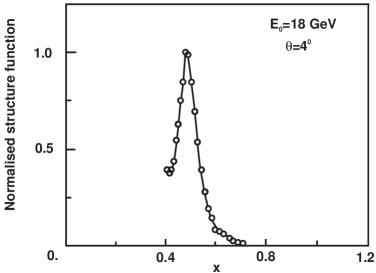
Figure 3: The structure function for quasi-elastic $e^{-}d$ scattering, see text

where the ”structure function” of the deuteron measured in quasi-elastic $e^{-}d$ scattering [11] is shown, clearly proving the presence of two nucleons in the nucleus. The similarity with general picture Fig.2 is well seen. The kinematics of the two nucleons in the deuteron rest system implies

$${\it\sqrt{m^{2}+\left|\overrightarrow{p_{1}}\right|^{2}}+\sqrt{m^{2}+\left|\overrightarrow{p_{2}}\right|^{2}}=M_{D},\qquad\overrightarrow{p_{1}}=-\overrightarrow{p_{2}}}$$ (4.1)

where $m$ should be understood as some effective mass which, due to binding is slightly less then $M_{D}/2$. This difference roughly corresponds to the depth of the potential if non-relativistic approach is used. From (4.1) the kinematically allowed region for corresponding $x$ easily follows

$$0.5-\Delta x\leq x\leq 0.5+\Delta x,\qquad\Delta x\equiv\frac{1}{2}\sqrt{1-\left(\frac{2m}{M_{D}}\right)^{2}}$$ (4.2)

In the case of partons inside the nucleon the situation is much more delicate. The interaction among the quarks and gluons is very strong, partons themselves are mostly in some shortly living virtual state, is it possible to speak about their mass at all? Strictly speaking probably not. The mass in exact sense is well defined only for free particles, whereas the partons are never free by definition. Therefore let us try to speak at least about an effective mass. By this term we roughly mean the mass that a free parton would have to have to interact with the probing lepton equally as our bounded one. Intuitively, this mass should correlate to $Q^{2}$. A lower $Q^{2}$ allows more time and space for struck parton to interact with some others, in the result the energy is transferred to a greater system than the parton itself. On the contrary, the higher $Q^{2}$ should mediate interaction with more ”isolated” parton.

Now let us try the formulae from previous section (with suggested sense of mass $m$) confront with the experimental data. In the Fig.4 recently obtained picture of the proton structure function $F_{2}$ [12] is shown.

Figure 4: The structure function $F_{2}(x,Q^{2})$ taken from [12].

No peak of that sort in Fig.2 or Fig.3 according to Eq.(3.57) is seen. There are two extreme alternatives.

1) The effective mass $m/M$ of quarks can be for given $Q^{2}$ well represented by one number. Then, obviously this value should be below the experimental limit of $x$ $\approx 10^{-3}\div 10^{-4}.$

2) The concept of effective mass reflects even for fixed $Q^{2}$ rather some distribution than a single value. Then the structure function is some superposition of curves similar to that in Fig.2 , but with different positions of their maxima. Such superposition could be generated not only by different flavors but also by the components commonly denoted by the term valence and sea quarks with distribution functions given e.g. in [13]. We shall not discuss the scenario of effective mass distribution in general, but only check one extreme: the case of static partons mentioned just below Eq.(3.38). These partons exactly obey the equation $p_{\alpha}=xP_{\alpha}$. Obviously having measured $F_{2}$ from the limit $x\geq L$, one can estimate the mean value

$$\frac{<m>}{M}<\frac{\int_{L}^{1}xF(x)dx}{\int_{L}^{1}F(x)dx}=\frac{\int_{L}^{1}F_{2}(x)dx}{\int_{L}^{1}\frac{F_{2}(x)}{x}dx}$$ (4.3)

The numerical calculation with the function fitting the data in the Fig.4

$$F_{2}(x,Q^{2})=[3.07x^{0.75}+0.14x^{-0.19}(1-2.93\sqrt{x})(\ln Q^{2}-0.05\ln{}^{2}Q^{2})](1-x)^{3.65}$$ (4.4)

gives the value $<m>$ in the region of tens $MeV$ depending on $L$ and $Q^{2}$ very roughly as

$$\frac{<m>}{M}<1.8\frac{L^{0.34}}{\ln Q^{2}},\qquad 10^{-4}\leq L\leq 10^{-2},\qquad 20\leq Q^{2}\leq 1600GeV^{2}$$ (4.5)

Obviously, this scenario is less restrictive than the first one.

It is possible, that the real case is somewhere between the two mentioned extremes. At the same time, the $Q^{2}$ dependence in Fig.4 could be qualitatively understood in the manner suggested above: the higher $Q^{2}$ prefers to mediate interactions with partons having less effective mass, therefore for higher $Q^{2}$ the low $x$ region should be more populated. Apparently, the quantitative expression of this correspondence is problem of dynamics.

5 Summary

In the present paper we have discussed a connection between the parton distribution functions ordinarily defined in the infinite momentum frame and the analogous functions defined in the hadron rest system. Assuming spherical symmetry of the hadron and an equal effective mass $m$ of the all partons of considered sort we have shown:

1) There exists unambiguous relation between the distribution functions defined in the both reference systems.

2) The proposed approach taking consistently parton transversal momenta into account gives the relation between the (electromagnetic) structure and distribution function somewhat modified in regard of the standard one. However, the standard relation is involved in that of our as a limiting case. The approach is not connected to any preferred reference system and explicitly involves ratio $m/M$ as a free parameter.

3) Within our approach in the structure functions we have identified some rather small, $Q^{2}$-dependent terms having purely kinematic origin.

4) The resulting relations pose the constraint on the shape of structure and distribution functions, which implies in particular the functions have the maximum at $x\approx m/M$ and vanish for $x<m^{2}/M^{2}.$

5) We compared our results with the data on proton structure function $(F_{2})$ assuming the two rather extreme scenarios:

i) The effective mass is for a fixed $Q^{2}$ well represented by one number, then the ratio $m/M$ is below presently reached limit of $x$ $(10^{-3}\div 10^{-4}).$

ii) The effective mass is at given $Q^{2}$ represented by some distribution and moreover the partons are static. Then the present data suggest the value $<m>/M$ should be at most of order $10^{-2}$.

Simultaneously, the $Q^{2}$ -dependence of structure function is qualitatively interpreted as a result of dynamic correlation of the effective mass and $Q^{2}$.

Acknowledgements I would like to express my gratitude to J.Pišút for many inspiring discussions which in the result motivated this work. I am also indebted to J.Chýla for critical reading of the manuscript and valuable comments.

References

• [1] Proceedings of the Int. Europhys. Conf. on High Energy Physics, Brussels 1995 (Editors: J.Lemonne, C.Vander Velde, F. Verbeure; World Scientific,1996).
• [2] J.Franklin, Phys.Rev.D16(1977),21.
• [3] J.Franklin, Nucl.Phys.B138(1978),122.
• [4] J.Franklin, M.Ierano, preprint TUHE-95-82, e-print:hep-ph/9508313.
• [5] J.Cleymans, R.L.Thews, Z.Phys.C37(1988),315.
• [6] R.S.Bhalerao, Phys.Lett.B380(1996),1; erratum - ibid.B387(1996),881.
• [7] R.P.Feynman, Photon - Hadron Interactions (W.A.Benjamin, Inc. 1972).
• [8] F.E.Close, An Introduction to Quarks and Partons (Academic, New York, 1979).
• [9] I.J.R.Aitchison, A.J.G.Hey, Gauge Theories in Particle Physics, 2nd edition (Adam Hilger, Bristol, 1989).
• [10] BCDMS Collaboration (A.C.Benvenuti et al.) Phys.Lett. B223(1989),485.
• [11] W.B.Attwood in Proc. 1979 SLAC Summer Institute on Particle Physics(SLAC-224) ed. A.Mosher, vol.3.
• [12] H1 Collaboration (T.Ahmed et al.) Nucl.Phys.B439(1995),471.
• [13] A.D.Martin, W.J.Stirling, R.G.Roberts, Phys.Rev.D50(1994),6734.