TUM-HEP-254/96 hep-ph/9609310

PHENOMENOLOGY OF $\mathbf{\varepsilon_{K}}$ IN THE TOP ERA
Ulrich Nierste, Physik-Department, TU München, D-85747 Garching, Germany

Abstract

Todays key information on the shape of the unitarity triangle is obtained from the well-measured quantity $\varepsilon_{K}$ characterizing the CP-violation in $\mathrm{|\Delta S|\!=\!2}$ transitions. The phenomenological analysis requires the input of four key quantities: The magnitudes of the CKM elements $V_{cb}$ and $V_{ub}$, the top quark mass and the non-perturbative parameter $B_{K}$. In the recent years all of them have been determined with increasing precision. In order to keep up with this progress the $\mathrm{|\Delta S|\!=\!2}$-hamiltonian had to be obtained in the next-to-leading order (NLO) of renormalization group improved perturbation theory. I present the NLO results for the QCD coefficients $\eta_{1}$ and $\eta_{3}$, which have been calculated by Stefan Herrlich and myself, and briefly sketch some aspects of the calculation. Then I give an update of the unitarity triangle using the summer 1996 data for the input parameters. The results for the improved Wolfenstein parameters $\overline{\rho}$ and $\overline{\eta}$ and the CKM phase $\delta$ are

$$-0.21\leq\overline{\rho}\leq 0.22,\qquad 0.27\leq\overline{\eta}\leq 0.43, \qquad 57^{\circ}\leq\delta\leq 122^{\circ}.$$

The range for the quantity $\sin(2\beta)$ entering CP asymmetries in B-decays is found as

$$0.46\;\leq \sin\left(2\beta\right) \leq\;0.79.$$

The given ranges correspond to one standard deviation in the input parameters. Finally I briefly discuss the $\mathrm{K_{L}\!-\!K_{S}}\,$-mass difference.

1 Motivation

$\varepsilon_{K}$ characterizes the CP-violation in the mixing of the neutral Kaon states $\mathrm{K^{0}}$ and $\mathrm{\overline{K^{0}}}$. This indirect CP-violation has been discovered in 1964 by Christenson, Cronin, Fitch and Turlay [1]. In the subsequent three decades refined experiments have reduced the error in $\varepsilon_{K}$ below 1% [2, 3], but yet no other CP-violating quantity has been unambiguously determined. In the Standard Model the only source of CP-violation is a complex phase $\delta$ in the Cabibbo-Kobayashi-Maskawa (CKM) matrix. Hence today the measured value of $\varepsilon_{K}$ plays the pivotal rôle in the determination of $\delta$. In the near future B-physics experiments will reveal whether the single parameter $\delta$ can simultaneously fit CP-violating observables in both the B- and the K- system and will eventually open the door to new physics.

The lowest order contribution to the $|\Delta S|\!=\!2$-amplitude inducing $\mathrm{K^{0}\!-\!\overline{K^{0}}}\,$-mixing is depicted in Fig. 1.

 

Figure 1: The lowest order box diagram mediating a $\mathrm{|\Delta S|\!=\!2}$ transition. The zigzag lines denote W-bosons or fictitious Higgs particles.

 

In order to calculate the Standard Model prediction for $\varepsilon_{K}$ one must first separate the short distance physics from long distance effects in the $\mathrm{|\Delta S|\!=\!2}$ transition amplitude. After successively integrating out the heavy degrees of freedom $m_{t}$, $M_{W}$ and $m_{c}$ one ends up with an effective low-energy $\mathrm{|\Delta S|\!=\!2}$-hamiltonian:

$$H^{|\Delta S|=2} = \frac{G_{F}^{2}}{16\pi^{2}}M_{W}^{2}\left[\lambda_{c}^{2}\eta_{1}^{\star}x_{c}^{\star}\!+\!\lambda_{t}^{2}\eta_{2}^{\star}S(x_{t}^{\star})\!+\!2\lambda_{c}\lambda_{t}\eta_{3}^{\star}S(x_{c}^{\star},x_{t}^{\star})\right]b(\mu)Q_{S2}(\mu)+\mathrm{h.c.}\;\;$$ (1)

Here $G_{F}$ is the Fermi constant, $M_{W}$ is the W boson mass, $\lambda_{j}=V_{jd}V_{js}^{*}$ comprises the CKM-factors and $Q_{S2}$ is the local $\mathrm{|\Delta S|\!=\!2}$ four-quark operator

$$Q_{S2} = \overline{s}_{j}\gamma_{\mu}(1-\gamma_{5})d_{j}\cdot\overline{s}_{k}\gamma^{\mu}(1-\gamma_{5})d_{k}$$ (2)

with $j$ and $k$ being colour indices. $x_{q}^{\star}=m_{q}^{\star\,2}/M_{W}^{2}$, where $m_{q}^{\star}=m_{q}(m_{q})$, $q=c,t$, are running quark masses in the $\overline{\mathrm{MS}}$ scheme. The Inami-Lim functions $S(x)$ and $S(x,y)$ contain the quark mass dependence of the box diagram in Fig. 1.

The short distance QCD corrections are comprised in the coefficients $\eta_{1}$, $\eta_{2}$ and $\eta_{3}$ with a common factor $b(\mu)$ split off. They are functions of the charm and top quark masses and of the QCD scale parameter $\Lambda_{\mathrm{QCD}}$. Further they depend on the definition of the quark masses used in the Inami-Lim functions: In (1) the $\eta_{i}$’s are defined with respect to $\overline{\mathrm{MS}}$ masses $m_{q}^{\star}$ and are therefore marked with a star. In the absence of strong interaction one has $\eta_{i}b(\mu)=1$.

$|\varepsilon_{K}|$ is proportional to the imaginary part of the hadronic matrix element $\langle\overline{K^{0}}\mid H^{\mathrm{|\Delta S|\!=\!2}}\mid{K^{0}}\rangle$. It thereby involves the hadronic matrix element of $Q_{S2}$ in (2), which is conveniently parametrized as

$$\langle\overline{K^{0}}\mid Q_{S2}(\mu)\mid{K^{0}}\rangle = \frac{8}{3}\frac{B_{K}}{b(\mu)}f_{K}^{2}m_{K}^{2}.$$ (3)

Here $m_{K}$ and $f_{K}$ are mass and decay constant of the neutral K meson and $\mu$ is the renormalization scale at which the short distance calculation of (1) is matched with the non-perturbative evaluation of (3). $B_{K}$ in (3) is defined in a renormalization group (RG) invariant way, because the $\mu$-dependent terms from (3) and (1) cancel in $\langle\overline{K^{0}}\mid H^{\mathrm{|\Delta S|\!=\!2}}\mid{K^{0}}\rangle$.

Now the CKM matrix depends on four independent parameters. The convenient Wolfenstein parametrization expands all CKM elements in terms of the well-known quantity $\lambda\simeq 0.22\simeq|V_{us}|$ to order $\lambda^{3}$. The proper study of CP violation, however, requires a higher accuracy [4, 5, 6]. The improved Wolfenstein approximation adopted in [5, 6] yields

$$V_{us}=\lambda+O\left(\lambda^{7}\right), \quad V_{cb}=A\lambda^{2}+O\left(\lambda^{8}\right),\qquad V_{ub}=A\lambda^{3}\left(\rho-i\eta\right).$$

From $b\rightarrow c$ decays one extracts $|V_{cb}|$ and thereby $A$. The information encoded in the remaining two parameters $(\rho,\eta)$ is traditionally depicted as a unitarity triangle in the complex plane. Two of its corners are located at $(0,0)$ and $(1,0)$, while the exact location $(\overline{\rho},\overline{\eta})$ of its top corner is defined by

$$\overline{\rho}\,+\,i\,\overline{\eta} = -\frac{V_{ud}V_{ub}^{*}}{V_{cd}V_{cb}^{*}}.$$ (4)

$\overline{\rho}$ and $\overline{\eta}$ are related to $\rho$ and $\eta$ by [5, 6]

$$\overline{\rho}=\rho\,\left(1-\frac{\lambda^{2}}{2}+O(\lambda^{4})\right), \overline{\eta}=\eta\,\left(1-\frac{\lambda^{2}}{2}+O(\lambda^{4})\right).$$

Inserting the improved Wolfenstein approximation into the expression for $|\varepsilon_{K}|$ yields

$$5.3\cdot 10^{-4}=B_{K}A^{2}\overline{\eta}\left[\left(1-\overline{\rho}+\Delta\left(\overline{\rho},\overline{\eta}\right)\right)A^{2}\lambda^{4}\eta^{\star}_{2}S(x^{\star}_{t})+\eta^{\star}_{3}S(x^{\star}_{c},x^{\star}_{t})-\eta^{\star}_{1}x^{\star}_{c}\right]\left(1+O\left(\lambda^{4}\right)\right).$$ (5)

In the absence of the small term

$$\Delta\left(\overline{\rho},\overline{\eta}\right) = \lambda^{2}\,\left(\overline{\rho}-\overline{\rho}^{2}-\overline{\eta}^{2}\right)$$ (6)

(5) defines a hyperbola in the $\left(\overline{\rho},\overline{\eta}\right)$-plane. The second input needed to determine the shape of the unitarity triangle is provided by the measured value of $|V_{ub}/V_{cb}|$, which fixes a circle in the $(\overline{\rho},\overline{\eta})$-plane:

$$\left|\frac{V_{ub}}{V_{cb}}\right| = \lambda\sqrt{\overline{\rho}^{2}+\overline{\eta}^{2}}\,\left(1+\frac{\lambda^{2}}{2}+O\left(\lambda^{4}\right)\right).$$ (7)

The intersection points of circle and hyperbola are the allowed values for $(\overline{\rho},\overline{\eta})$ (see Fig. 2).

 

Figure 2: The two solutions for $(\bar{\rho},\bar{\eta})$ are the intersections of the hyperbola from $\varepsilon_{K}$ with the circle obtained from $|V_{ub}|/|V_{cb}|$. The plot also visualizes the impact of the NLO calculation of $\eta_{3}$ on the unitarity triangle: For the chosen set of input parameters the LO value for $\eta_{3}$ yields no solution for $(\bar{\rho},\bar{\eta})$.

 

The standard phenomenological analysis of $\varepsilon_{K}$ involves four key input parameters: The hyperbola (5) is entered by $B_{K}$, $m_{t}$ and (via $A$) $|V_{cb}|$ and the circle involves $|V_{ub}/V_{cb}|$. In the past few years significant progress has been made in the determination of these quantities:

• $|V_{cb}|$: Both exclusive and inclusive $b\rightarrow c\ell\nu_{\ell}$ decays have been precisely measured by CLEO and ALEPH. The theoretical extraction of $|V_{cb}|$ from the decay rates has been refined by the development of heavy quark effective theory and today we know $|V_{cb}|$ to 8 % accuracy.

• $|V_{ub}/V_{cb}|$: In addition to inclusive measurements of $b\rightarrow u\ell\nu_{\ell}$ decays now also the exclusive decays $B\rightarrow\rho\ell\nu_{\ell}$ and $B\rightarrow\pi\ell\nu_{\ell}$ have been measured by CLEO.

• $B_{K}$: The lattice results have steadily improved as reported by G. Kilcup at this workshop.

• $m_{t}$: Most importantly the top quark has been discovered at FERMILAB. In the time before the top discovery the unknown value of $m_{t}$ was the largest source of uncertainty in the phenomenology of $\varepsilon_{K}$. Now in the top era the experimental error in $m_{t}$ affects the determination of the unitarity triangle less than those in the other three input parameters.

Clearly the accuracy of the QCD coefficients $\eta_{1}$, $\eta_{2}$ and $\eta_{3}$ of $H^{|\Delta S|=2}$ entering the hyperbola (5) must keep up with this progress! This has required to calculate them in the next-to-leading order (NLO) of renormalization group (RG) improved perturbation theory.

2 $\mathbf{H^{|\Delta S|=2}}$ in the next-to-leading order

Suppose one would try to determine the strength of $\mathrm{|\Delta S|\!=\!2}$ transitions simply by calculating the box diagram of Fig. 1 and its dressing with gluons. This would result in a very poor description of $\mathrm{K^{0}\!-\!\overline{K^{0}}}\,$-mixing for various reasons: First long-distance QCD is non-perturbative and therefore cannot be described by the exchange of gluons. Second the true external states are mesons rather than quarks. Third the largely separated mass scales in the problem induce large logarithms in the radiative corrections: For example the QCD corrections to the box diagram with two internal charm quarks contain $(\alpha_{s}/\pi)\ln x_{c}\simeq 1$, which spoils perturbation theory. Fourth one faces a scale ambiguity for the same reason: Should one evaluate the running coupling $\alpha_{s}$ at the scale $\mu=M_{W}$, $\mu=m_{c}$ or any scale in between? These problems can be overcome with the help of Wilson’s operator product expansion, which expresses the Standard Model amplitudes of interest in terms of an effective hamiltonian, in which the fields describing heavy particles such as W-boson and top-quark do not appear anymore. Instead the transitions mediated by them are described by effective operators, which can be obtained from the Standard Model diagrams by contracting the heavy lines to a point. E.g. contracting the top-quark and the W-boson lines in Fig. 1 yields the four-quark operator $Q_{S2}$ in (2). The operators are multiplied by short distance Wilson coefficients, which are functions of the heavy masses. Disturbingly large logarithms can then be summed to all orders by applying the RG to the coefficients. Starting with the heaviest masses $m_{t}$ and $M_{W}$, the whole procedure is then repeated with the next lighter particle, in our case the charm quark. Finally in $H^{|\Delta S|=2}$ the coefficient of the operator $Q_{S2}$ is rewritten in terms of the Inami-Lim functions and the $\eta_{i}$’s.

The minimal way to incorporate short distance QCD effects is the leading logarithmic approximation. For example the leading order (LO) expression for $\eta_{1}\cdot x_{c}$ contains the result of the box diagram in Fig. 1 with two internal charm quarks and the large logarithmic term $[\alpha_{s}\ln x_{c}]^{n}$ to all orders $n=0,1,2,\ldots$ of the perturbation series. The NLO improves the LO results by including those terms with an additional factor of $\alpha_{s}$, in the case of $\eta_{1}$ these are the results of the two-loop diagrams with an additional gluon dressing the box and the summation of $\alpha_{s}[\alpha_{s}\ln x_{c}]^{n}$, $n=0,1,2,\ldots$. In the modern formalism described in the first paragraph the LO $\eta_{i}$’s have been calculated by Gilman and Wise in 1983 [7] partly confirming earlier results obtained with different methods. Yet in general LO results suffer from various conceptual drawbacks. In the case of the $\eta_{i}$’s one faces four problems:

• The LO results do not reproduce the correct dependence on $m_{t}$. Especially the dependence of $\eta_{3}$ on $m_{t}$ enters in the NLO.

• Likewise the proper definition of $m_{t}$ is a NLO issue. One must go to the NLO to learn how to use the FERMILAB measurement of the pole quark mass $m_{t}^{\mathrm{pole}}$ in a low energy hamiltonian like $H^{|\Delta S|=2}$ in (1). In a NLO expression it is appropriate to use the one-loop formula to relate $m_{t}^{\mathrm{pole}}$ to $m_{t}^{\star}$ entering $H^{|\Delta S|=2}$. These two definitions $m_{t}^{\mathrm{pole}}$ and $m_{t}^{\star}$ differ by 8 GeV, which is more than the present experimental error in $m_{t}^{\mathrm{pole}}$.

• The fundamental QCD scale parameter $\Lambda_{\overline{\mathrm{MS}}}$ is an essential NLO quantity and cannot be used in LO expressions.

• The LO results for $\eta_{1}$ and $\eta_{3}$ suffer from large renormalization scale uncertainties. Their reduction requires a NLO calculation.

The coefficient $\eta_{2}$ has been calculated in the NLO by Buras, Jamin and Weisz [8]. The NLO order results for $\eta_{1}$ [9] and $\eta_{3}$ [6, 10] have been derived by Stefan Herrlich and myself.

The three results read

$$\eta_{1}^{\star} = 1.31\raisebox{-2.15277pt}{\shortstack[l]{$\scriptstyle+0.25$\\ $\scriptstyle-0.22$}}\,,\quad\quad\eta_{2}^{\star}\;=\;0.57\raisebox{-2.15277pt}{\shortstack[l]{$\scriptstyle+0.01$\\ $\scriptstyle-0.01$}}\,,\quad\quad\eta_{3}^{\star}\;=\;0.47\raisebox{-2.15277pt}{\shortstack[l]{$\scriptstyle+0.03$\\ $\scriptstyle-0.04$}}\,.$$ (8)

The coefficients are scheme independent except that they depend on the definition of the quark masses in $H^{\mathrm{|\Delta S|\!=\!2}}$. The errors are estimated from the remaining scale uncertainty. $\eta_{2}^{\star}$ and $\eta_{3}^{\star}$ depend on $\alpha_{s}$ and the quark masses only marginally. The quoted value for $\eta_{1}^{\star}$ corresponds to $m_{c}^{\star}=1.3\,\mathrm{GeV}$ and $\alpha_{s}(M_{Z})=0.117\,\mathrm{GeV}$. For other values of $\alpha_{s}$ and $m_{c}^{\star}$ see the tables in [9, 10].

The NLO values in (8) have to be compared with the old LO results:

$$\eta_{1}^{\mathrm{LO}} \approx 0.74\,,\quad\quad\eta_{2}^{\mathrm{LO}}\approx 0.59\,,\quad\quad\eta_{3}^{\mathrm{LO}}\approx 0.37\,.$$ (9)

If one takes the difference between (9) and (8) as an estimate of the inaccuracy of the LO expressions, one finds that the use of the $\eta_{i}^{\mathrm{LO}}$’s in (5) imposes an error onto the phenomenological analysis of $\varepsilon_{K}$ which is comparable in size to the error stemming from the hadronic uncertainty in $B_{K}$.

I close the theoretical part of my talk by briefly sketching some details of the calculation of $\eta_{1}$ and $\eta_{3}$: The new feature compared to other NLO calculations was the appearance of two-loop diagrams with the insertion of two $\mathrm{|\Delta S|\!=\!1}$ operators. Pictorially they are obtained by contracting the W-lines in Fig. 1 to a point and dressing the diagram with gluons. Here the proper renormalization of such Green’s functions with two operator insertions had to be worked out [10]. This has required the correct renormalization of so called evanescent operators, which appear in the context of dimensional regularization [11]. Such operators induce a new type of scheme dependence into the calculation, which of course cancels in physical observables [11, 10].

3 1996 phenomenology of $\mathbf{\varepsilon_{K}}$ and the $\mathbf{K_{L}\!-\!K_{S}}\,$-mass difference

The first phenomenological analysis of $\varepsilon_{K}$ with NLO precision has been presented in [6]. In [6] $\overline{\rho}$ and $\overline{\eta}$ defined in (4), the CKM phase $\delta$ and other quantities related to the CKM matrix are tabulated as a function of $B_{K}$, $m_{t}$, $|V_{cb}|$ and $|V_{ub}/V_{cb}|$. Here I will update the unitarity triangle with the actual values of these key input parameters.

 

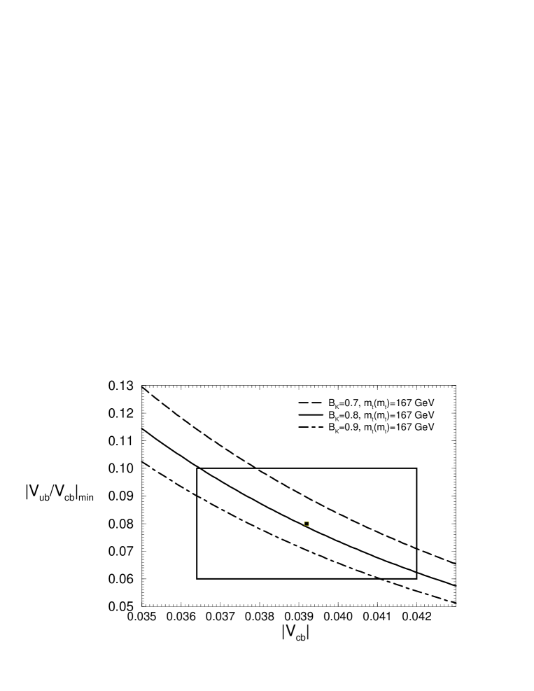
Figure 3: Borderline of new physics: For each pair $(m_{t}^{\star},B_{K})$ the measured value for $\varepsilon_{K}$ defines a curve. The points below the curve are excluded, if $\varepsilon_{K}$ is solely due to Standard Model physics. The rectangle shows the limits in (10) for $|V_{cb}|$ and $|V_{ub}/V_{cb}|$ obtained from tree-level b-decays. The central values used in the analysis are marked with the small filled square.

 

The existence of a solution for $(\overline{\rho},\overline{\eta})$ requires that the hyperbola in (5) intersects or at least touches the circle defined in (7) as shown in Fig. 2. This feature yields lower bounds on each of the four input parameters as a function of the other three ones. In Fig. 3 this condition is displayed as a constraint on the CKM elements. The present status of the unitarity triangle is shown in Fig. 4.

 

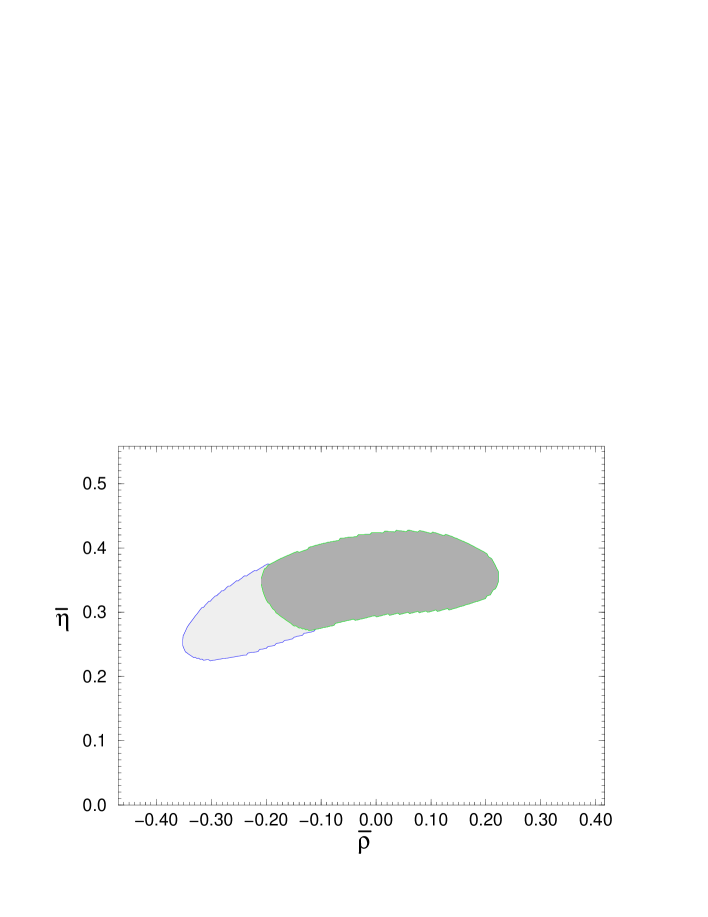
Figure 4: The allowed region for the top $(\overline{\rho},\overline{\eta})$ of the unitarity triangle: The dark shade denotes the area which is simultaneously allowed by $\varepsilon_{K}$ and ${B^{0}\!-\!\overline{B^{0}}}\,$-mixing. The light gray area complies with $\varepsilon_{K}$, but not with $\Delta m_{B_{d}}$. The impact of the limit on $\Delta m_{B_{s}}$ is discussed in the text.

 

The input parameters are taken as [12]

$$|V_{cb}|=0.0392\pm 0.0028,\quad\left|\frac{V_{ub}}{V_{cb}}\right|=0.08\pm 0.02,\quad m_{t}^{\star}=(167\pm 6)\,\mathrm{GeV},\quad B_{K}=0.8\pm 0.1.$$ (10)

Here $|V_{cb}|$ is extracted from an analysis of exclusive semileptonic B-decays. The quoted value for $m_{t}^{\star}$ corresponds to $m_{t}^{\mathrm{pole}}=(175\pm 6)\,\mathrm{GeV}$. The range for $B_{K}$ includes the ballpark of the lattice results presented in [12, 13] and the result of the $1/N_{c}$ expansion in [14].

Next we include the experimental information from $\mathrm{B^{0}\!-\!\overline{B^{0}}}\,$-mixing into our analysis: The ALEPH results [12]

$$\Delta m_{B_{d}}=(0.464\pm 0.018)\,\mathrm{ps}^{-1}=(305\pm 12)\,\mu\mathrm{eV}, \qquad\Delta m_{B_{s}}>9.2\,\mathrm{ps}^{-1},$$ (11)

exclude a part of the region allowed by $\varepsilon_{K}$. The measured value of $\Delta m_{B_{d}}$ constrains the distance of $(\overline{\rho},\overline{\eta})$ to the point $(1,0)$:

$$(1-\overline{\rho})^{2}+\overline{\eta}^{2} = \frac{4.76\cdot 10^{8}\,\mathrm{GeV}\,\cdot\,\Delta m_{B_{d}}}{B_{B_{d}}\,F_{B_{d}}^{2}\,S(x_{t}^{\star})\,|V_{cb}|^{2}}.$$ (12)

In Fig. 4 we have used [12, 15]

$$F_{B_{d}}=(175\pm 30)\mathrm{MeV},\quad \qquad B_{B_{d}}=1.31$$ (13)

and the central value for $\Delta m_{B_{d}}$ in (11). The variation of 30 MeV in $F_{B_{d}}$ accounts for the actual error of 25 MeV and the smaller errors in $B_{B_{d}}$ and $\Delta m_{B_{d}}$ reported in [12]. The whole shaded area in Fig. 4 shows the region which is allowed from the analysis of $\varepsilon_{K}$ alone. The analysis of $\varepsilon_{K}$ is not particularly sensitive to the treatment of the errors in (10). In Fig. 4 they have been treated statistically: Setting $(x_{1},x_{2},x_{3},x_{4})=(|V_{cb}|,|V_{ub}/V_{cb}|,m_{t}^{\star},B_{K})$ and denoting their central values by $\overline{x}_{i}$ and their errors by $\Delta x_{i}$ the $x_{i}$’s have been restricted to the $1\sigma$-ellipsoid $\sum_{i}(x_{i}-\overline{x}_{i})^{2}/(\Delta x_{i})^{2}\leq 1$. The error in the analysis of $\Delta m_{B_{d}}$ is theoretical and therefore treated non-statistically: For each point $(\overline{\rho},\overline{\eta})$ it has been checked whether it corresponds to a value of $F_{B_{d}}$ in the range given in (13). Finally the bound for $\Delta m_{B_{s}}$ also excludes a part of the light gray area, but it does not further constrain the dark region allowed from both $\varepsilon_{K}$ and $\Delta m_{B_{d}}$, if one uses $F_{B_{s}}/F_{B_{d}}=1.25\pm 0.10$, which one expects from an unquenched lattice calculation [12]. Yet future tighter bounds on $\Delta m_{B_{s}}$ will give extra information on the unitarity triangle [16]. From the result for $(\overline{\rho},\overline{\eta})$ one can extract the CKM phase $\delta$. Another interesting quantity is $\sin(2\beta)$, where $\beta$ is the angle of the unitarity triangle adjacent to the corner $(1,0)$. $\sin(2\beta)$ enters CP asymmetries in B-decays. One finds

$$57^{\circ}\leq\delta\leq 122^{\circ}, \qquad 0.46\leq\sin\left(2\beta\right)\leq 0.79.$$ (14)

The coefficient $\eta_{1}$ is known less accurately than $\eta_{2}$ and $\eta_{3}$ due to the sizeable scale uncertainty in (8) and its strong dependence on $\alpha_{s}$. Fortunately the term involving $\eta_{1}$ in (5) is of minor importance for the analysis of $\varepsilon_{K}$. In contrast the short distance part of the $\mathrm{K_{L}\!-\!K_{S}}\,$-mass difference, which is obtained from the real part of $\langle\overline{K^{0}}\mid H^{\mathrm{|\Delta S|\!=\!2}}\mid{K^{0}}\rangle$, is dominated by $\eta_{1}$ and therefore plagued by theoretical uncertainties. With $B_{K}$ in (10) and $\alpha_{s}(M_{Z})=0.118\pm 0.004$ the ratio of the short distance part of $\Delta m_{K}$ and its experimental result [3, 17] reads

$$\frac{\left(\Delta m_{K}\right)_{\mathrm{SD}}}{\left(\Delta m_{K}\right)_{\mathrm{exp}}} = 0.74\raisebox{-2.15277pt}{\shortstack[l]{$\scriptstyle+0.25$\\ $\scriptstyle-0.20$}}.$$ (15)

At least this reveals a short distance dominance of $\Delta m_{K}$ in accordance with the expectations from power counting [9, 6].

Acknowledgements

I am grateful to the organizers for the invitation and a supporting grant allowing me to attend this excellent workshop. During this conference I have enjoyed many stimulating discussions, especially with Stefano Bertolini, Eduardo de Rafael, Jean-Marc Gérard, Fred Gilman and Guido Martinelli. Section 3 has benefited from discussions with Andrzej Buras, Stefan Herrlich and Weonjong Lee.

References

-
[1]
J. H. Christenson, J. W. Cronin,
V. L. Fitch and R. Turlay,
Phys. Rev. Lett. 13 (1964) 138.
J. H. Christenson, J. W. Cronin, V. L. Fitch and R. Turlay, Phys. Rev. 140B (1965) 74. - [2] CPLEAR collaboration, R. Adler et al., Phys. Lett. B363 (1995) 243.
- [3] Particle Data Group, Phys. Rev. D54 (1996) 1.
- [4] M. Schmidtler and K. Schubert, Z. Phys. C53 (1992) 347.
- [5] A. J. Buras, M. E. Lautenbacher and G. Ostermaier, Phys. Rev. D50 (1994) 3433.
- [6] S. Herrlich und U. Nierste, Phys. Rev. D52 (1995) 6505.
- [7] F. J. Gilman and M. B. Wise, Phys. Rev. D27 (1983) 1128.
- [8] A. J. Buras, M. Jamin and P. H. Weisz, Nucl. Phys. B347 (1990) 491.
- [9] S. Herrlich und U. Nierste, Nucl. Phys. B419 (1994) 292.
- [10] S. Herrlich und U. Nierste, The Complete -Hamiltonian in the Next-To-Leading Order, Nucl. Phys. B, in press, hep-ph/9604330.
- [11] S. Herrlich und U. Nierste, Nucl. Phys. B455 (1995) 39.
- [12] Talks by P. Tipton, J. Flynn and L. Gibbons at the 28th Int. conference on high energy physics, Warsaw, Poland, July 1996.
- [13] W. Lee and M. Klomfass, hep-lat/9608089.
-
[14]
W. A. Bardeen, A. J. Buras and J.-M. Gérard,
Phys. Lett. B211 (1988) 343.
J.-M. Gérard, Acta Phys. Pol. B21 (1990) 257. -
[15]
C. R. Allton, M. Ciuchini, M. Crisafulli, V. Lubicz and
G. Martinelli,
Nucl. Phys. B431 (1994) 667. -
[16]
G. Buchalla, A. J. Buras and M. E. Lautenbacher,
hep-ph/9512380.
A. Ali and D. London, hep-ph/9607392. - [17] CPLEAR collaboration, R. Adler et al., Phys. Lett. B363 (1995) 237.