Nonfactorizable QCD and Electroweak Corrections to the Hadronic
$Z$ Boson Decay Rate

Abstract

We present an analysis of two-loop mixed QCD and electroweak corrections to the decay of the $Z$ boson into light quarks. We find that the naive factorization of QCD and electroweak corrections does not describe correctly the two-loop effects. The nonfactorizable corrections shift the width of the $Z$ boson by approximately $-0.55(3)$ MeV and increase the central value of the strong coupling constant determined at LEP by 0.001.

With a total number of about four million hadronic $Z$ decays collected at each of the four LEP experiments a final precision in the $Z$ boson decay rate of about 2 MeV is expected. At the same time the ratio $R_{\rm had}=\Gamma(Z\to{hadrons})/\Gamma(Z\to\mu^{+}\mu^{-})$ will be measured with an accuracy of about 0.1 per cent. These measurements will determine $\alpha_{s}$ with a remaining uncertainty of about $\delta\alpha_{s}=\pm 3\times 10^{-3}$. This puts not only severe constraints on the experimental analysis but also on the theoretical understanding of subtle higher order effects. QCD corrections have been calculated up to order $\alpha_{s}^{3}$ [1] and leading as well as subleading electroweak corrections have been calculated up to two loops [2].

Another important class of effects is provided by the interplay between electroweak interactions and QCD. The relation between $M_{W}$, $M_{Z}$, $G_{F}$, and $\alpha$ is affected by the large top quark mass and again two and even three loop self-energies have been evaluated to arrive at accurate predictions. In addition there is of course the large class of “reducible” corrections which originate from one-loop electroweak diagrams, multiplied by the QCD correction factor $(1+\alpha_{s}/\pi)$. The remaining two-loop effects are induced by nonfactorizable vertex corrections. With an order of magnitude of ${\alpha_{\rm weak}\over\pi}{\alpha_{s}\over\pi}\approx 0.4\times 10^{-3}$ and an unknown coefficient, they are not a priori negligible for an analysis at the 0.1 per cent level. In particular it is evident that an ansatz assuming factorization between QCD and weak effects cannot be valid for the irreducible vertex diagrams. For the $Z$ decay rate into bottom quarks this has been confirmed by the calculation of the leading contributions which are enhanced by a factor $m_{t}^{2}/m_{W}^{2}$ [3, 4, 5, 6] and by logarithms $\ln(m_{t}^{2}/m_{W}^{2})$ [7, 8]. In both cases factorization is invalidated and nontrivial additional terms are obtained.

These results were derived by expanding in the “small” parameter $m_{W}^{2}/m_{t}^{2}$. In contrast, no such expansion parameter is available for the $Z$ decay rate into light $u$, $d$, $s$, or $c$ quarks. All these quarks are effectively massless and both $Z$ and $W$ bosons appear as virtual particles in the relevant vertex diagrams which have to be evaluated at $q^{2}=m_{Z}^{2}$. A similar problem arises also for the non-enhanced contributions to the $b\bar{b}$ vertex. However, the $Z$ decay rate is dominated by the $u$, $d$, $s$, and $c$ channels and the corresponding mixed terms will dominate in the total $Z$ decay rate. For this reason we concentrate on light quark final state.

The case of QCD combined with QED provides an illustrative example for mixed QCD-electroweak corrections. The factorization ansatz $\left(1+Q_{q}^{2}{3\over 4}{\alpha\over\pi}\right)\left(1+{\alpha_{s}\over\pi}\right)$ implies a mixed term $Q_{q}^{2}{3\over 4}{\alpha\over\pi}{\alpha_{s}\over\pi}$. However, the proper evaluation [9] leads to $-{1\over 3}Q_{q}^{2}{3\over 4}{\alpha\over\pi}{\alpha_{s}\over\pi}$, which differs in magnitude and sign from the naive ansatz.

With this motivation in mind we have evaluated the mixed corrections of order ${\alpha_{\rm weak}\over\pi}{\alpha_{s}\over\pi}$ for $\Gamma_{u}$ and $\Gamma_{d}$ which originate from irreducible vertex diagrams. Our approach is based on the observation that the relevant rates can be calculated for the decay of a virtual $Z$ with mass squared equal $q^{2}$, with $q^{2}$ alternatively far smaller or far larger than $m_{Z}^{2}$, by computing a large number of terms in the expansion in $q^{2}/m_{Z}^{2}$ or $m_{Z}^{2}/q^{2}$. The results can then be extrapolated even to $q^{2}=m_{Z}^{2}$.

The tree-level decay width of the $Z$ boson into light quarks is given by

$$\Gamma^{(0)}(Z\to q\bar{q}) = {\alpha N_{C}M_{Z}\over 6}\left[(g_{q}^{+})^{2}+(g_{q}^{-})^{2}\right]$$ (1)

$$g^{+}_{q} = -{s_{W}\over c_{W}}Q_{q}$$ (2)

$$g^{-}_{q} = {1\over s_{W}c_{W}}(I_{3q}-s_{W}^{2}Q_{q})$$ (3)

where $s_{W}$ and $c_{W}$ are sine and cosine of the weak mixing angle, $I_{3q}$ and $Q_{q}$ denote the isospin and electric charge of the quark $q$, and $N_{C}=3$ is the number of colors.

The Born level result (1) receives both QCD and electroweak corrections. The QCD corrections have been calculated up to three loops and yield a correction factor

$$\Gamma^{QCD}=\Gamma^{(0)}\left(1+{\alpha_{s}\over\pi}+\ldots\right)$$ (4)

First order electroweak corrections to the $Z$ boson hadronic width can be divided up into three finite parts

$$\Gamma^{\rm(1\ loop\ EW)}(Z\to q\bar{q})\equiv\Gamma^{Z}+\Gamma^{W}+\Gamma^{ct}$$ (5)

The first two contributions can be calculated from the imaginary parts of the on-shell self-energy diagrams shown in fig. (1). $\Gamma^{Z}$ is given by the vertex correction (1a) with a $Z$ boson exchange together with the $Z$ boson contribution to the wave function renormalization of the quarks (1b). $\Gamma^{W}$ is given by two analogous diagrams with the internal $Z$ boson replaced by $W$, plus the diagram (1c). In the linear ’t Hooft-Feynman gauge, adopted in this paper, the sum of those three diagrams is ultraviolet divergent. It is made finite by including in $\Gamma^{W}$ the divergent part of the counterterm generated by the $Z$ boson wave function renormalization; this is obtained by making the following replacements in the $Zq\bar{q}$ vertex:

$$g^{+}_{q}\to 0,\qquad g^{-}_{q}\to-{\alpha\over 4\pi}\left({1\over\varepsilon}-\ln M_{W}^{2}\right){2c_{W}\over s_{W}^{3}}I_{3q}.$$ (6)

(The calculation is done using dimensional regularization in $4-2\varepsilon$ dimensions.)

Finally, $\Gamma^{ct}$ is the tree-level decay width (1) multiplied by the remaining, finite $Z$ boson wave function renormalization constant.

The splitting of the decay rate into the three contributions is convenient for the description of the QCD corrections. In particular, the effect of QCD corrections on $\Gamma^{ct}$ is just the multiplicative factor given in eq. (4). For the remaining two contributions to the decay $Z\to q\bar{q}$ we have

$$\Gamma^{Z} = {\alpha^{2}N_{C}M_{Z}\over 12\pi}\left[(g_{q}^{+})^{4}+(g_{q}^{-})^{4}\right]\Lambda_{2}(x)$$ (7)

$$\Gamma^{W} = {\alpha^{2}N_{C}M_{Z}\over 24\pi s_{W}^{2}}g_{q}^{-}\left[g_{\tilde{q}}^{-}\Lambda_{2}(x)+6I_{3q}{c_{W}\over s_{W}}\Lambda_{3}(x)\right]$$ (8)

$$x = {s\over M^{2}}$$ (9)

where $\tilde{q}$ is the isospin partner of the quark $q$, $s$ is the momentum squared of the external $Z$ boson, and $M$ is the mass of the virtual heavy boson inside the diagram. For a decay of an on-shell $Z$ boson we have $x=1$ in $\Gamma^{Z}$ and $x=M_{Z}^{2}/M_{W}^{2}\approx 1.292$ in $\Gamma^{W}$. The functions $\Lambda_{2,3}$ can be expanded in a series in the strong coupling constant

$$\Lambda_{i}=\Lambda_{i}^{(0)}+C_{F}{\alpha_{s}\over\pi}\Lambda_{i}^{(1)}+\ldots$$ (10)

where $C_{F}=4/3$ is the $SU(3)$ color factor. The 0th order terms of these series have been calculated in [10, 11]

$$\Lambda_{2}^{(0)}(x) = -{7\over 2}-{2\over x}+\left({2\over x}+3\right)\ln x$$ (12)

$$-2\left({1+x\over x}\right)^{2}\left[\ln x\ln(1+x)+{\rm Li}_{2}(-x)\right]$$

$$\Lambda_{3}^{(0)}(x) = {5\over 6}-{2\over 3x}+{4+2x\over 3x}\sqrt{{4\over x}-1}\arctan{1\over\sqrt{{4\over x}-1}}$$ (14)

$$-{8\over 3}{2x+1\over x^{2}}\arctan^{2}{1\over\sqrt{{4\over x}-1}}$$

The behavior of these functions at $x\to 0$ and at $x\to\infty$ can be found from asymptotic expansions for small and large external momentum. It turns out that only the first few terms are needed to compute with good accuracy $\Lambda_{i}^{(0)}$ for all values of the argument $x$. This observation is the basis of the present paper. Since virtual gluons do not radically change the analytical properties of the $Z$ self-energy diagrams we can approximate the QCD correction functions $\Lambda_{i}^{(1)}$ by the first few terms of their asymptotic expansion. In a large part of the computations we employ the program package MINCER [12] written in FORM [13].

The function $\Lambda_{2}^{(1)}$ receives contributions from the diagrams shown in fig. (2) and fig. (3). If the virtual particle is the $Z$ boson the sum of these diagrams is finite. On the other hand, in the case of the virtual $W$ boson, the finite result is obtained only in the sum with the diagrams of fig. (4) and the counterterm discussed before eq. (6). This is a consequence of the difference between the $Z$ couplings to the quarks in diagrams 1a and 1b.

We notice, however, that the diagrams in fig. (3) are proportional to $(g^{-}_{q})^{2}$ which can be rewritten as $g^{-}_{q}g^{-}_{\tilde{q}}+2I_{3q}g^{-}_{q}c_{W}/s_{W}$. It is convenient to treat the two parts of this sum separately. The first part together with diagrams of fig. (2) is finite and gives a contribution described by $\Lambda_{2}^{(1)}$. The second part can be combined with diagrams in fig. (4) and the counterterm to give $\Lambda_{3}^{(1)}$.

We can write down an expansion of $\Lambda_{2}^{(1)}(x)$ around $x=0$ as a sum of three series

$$\Lambda_{2}^{(1)}(x)=S^{S}(x)+S^{V}_{1}(x)+S^{V}_{2}(x)\zeta(3)$$ (15)

The first series is obtained from the finite part of the corrections to the heavy boson contribution to the quark wave function renormalization, fig. (3). The remaining two series describe the gluonic effects on the heavy boson vertex correction shown in fig. (2); it is convenient to isolate the terms containing $\zeta(3)$. The results are

$$S^{S}(x)=\left[-{121\over 81}-{1\over 9}\ln^{2}(x)+{22\over 27}\ln(x)\right]x$$ (19)

$$+\left[-{169\over 5184}-{1\over 144}\ln^{2}(x)+{13\over 432}\ln(x)\right]x^{2}$$

$$+\left[-{2209\over 810000}-{1\over 900}\ln^{2}(x)+{47\over 13500}\ln(x)\right]x^{3}$$

$$+\left[-{1369\over 3240000}-{1\over 3600}\ln^{2}(x)+{37\over 54000}\ln(x)\right]x^{4}+{\cal O}(x^{5})$$

$$S^{V}_{1}(x)=\left[{71\over 18}-{1\over 2}\ln^{2}(x)-\ln(x)\right]x$$ (28)

$$+\left[-{1159\over 1728}-{7\over 24}\ln^{2}(x)+{5\over 4}\ln(x)\right]x^{2}$$

$$+\left[-{1853\over 7200}-{13\over 60}\ln(x)\right]x^{3}$$

$$+\left[+{146179\over 648000}-{11\over 120}\ln^{2}(x)+{83\over 540}\ln(x)\right]x^{4}$$

$$+\left[-{78941\over 396900}-{37\over 1890}\ln(x)\right]x^{5}$$

$$+\left[+{514328497\over 3556224000}-{143\over 3360}\ln^{2}(x)+{221\over 8640}\ln(x)\right]x^{6}$$

$$+\left[-{262758413\over 2286144000}-{1\over 720}\ln^{2}(x)+{799\over 90720}\ln(x)\right]x^{7}$$

$$+\left[+{13907067061\over 160030080000}-{403\over 16800}\ln^{2}(x)+{853\over 4536000}\ln(x)\right]x^{8}$$

$$+{\cal O}(x^{9})$$

$$S^{V}_{2}(x)=-2x+{1\over 2}x^{2}-{1\over 5}x^{3}+{1\over 10}x^{4}$$ (30)

$$\qquad-{2\over 35}x^{5}+{1\over 28}x^{6}-{1\over 42}x^{7}+{1\over 60}x^{8}+{\cal O}(x^{9})$$

In $S_{1}^{V}$ and $S^{S}$ we have not displayed terms ${\cal O}(x^{0})$ which are divergent but cancel in the sum.

$S^{S}$ and $S^{V}_{2}$ converge rapidly; in fact one can recognize the general formula for their coefficients and sum up both series exactly; the result (being a rather complicated function containing tetralogarithms) will be presented elsewhere.

On the other hand, $S_{1}^{V}$ converges very slowly for $x>1$; this is a consequence of a three-particle cut at $s=M_{Z}^{2}$ in the diagrams in fig. (2). This cut corresponds to the decay channel $Z\to W^{+}d\bar{u}$. If the internal heavy particle is a $W$ boson we need the value of this series at $x=1.292$. It is therefore necessary to compute the expansion of the function $\Lambda_{2}^{(1)}$ on the other side of the three-particle cut, that is the asymptotic behavior at $x\to\infty$. In analogy with eq. (15) we define

$$\Lambda_{2}^{(1)}(x)=T^{S}(1/x)+T^{V}_{1}(1/x)+T^{V}_{2}(1/x)\zeta(3)$$ (31)

In the sum $T^{S}+T^{V}_{1}$ the divergences cancel and the first three terms give

$$-{3\over 8}\left(1-{1\over x^{2}}\right).$$ (32)

We do not present here the full formulas for the $T$-series for the following reason: beginning with the term $1/x^{4}$, the coefficients of $1/x^{n}$ are identical (up to the sign of the logs) to the coefficients of $x^{n-2}$ in the corresponding series $S$. Also in the terms $1/x^{3}$ and $x$ there is an equality in the sums $T^{S}+T^{V}_{1}$ and $S^{S}+S^{V}_{1}$. This remarkable feature gives us confidence in the result. It should be stressed that the $S$ and $T$ series result from very different calculations.

The equality of the coefficients guarantees that both expansions give equal results at $x=1$. However, the slope of both approximations is not quite the same at $x=1$; we can take the magnitude of the resulting cusp as an estimate of the numerical error in the final result.

We also notice that values of $\Lambda_{2}^{(1)}$ at $x\approx 1$, relevant for the mixed QCD/electroweak corrections, are well approximated by the asymptotic value $\Lambda_{2}^{(1)}(x\to\infty)=-3/8$, which corresponds to the two loop mixed QCD/QED calculation [9]. We use in the numerical analysis $\Lambda_{2}^{(1)}(1)\approx\Lambda_{2}^{(1)}(1.292)\approx-0.37\pm 0.04$.

The calculation of $\Lambda_{3}^{(1)}$ involves four three-loop diagrams shown in fig. (4). In the present analysis of the QCD corrections we neglect the influence of the real $W$ emission [14, 15, 16]. (We notice that a part of it, originating from $W$ emission off quarks, has been included in the $T$ series discussed above. In principle this partial treatment is not gauge invariant; the induced error is, however, negligible due to the phase space suppression of the $W$ emission.)

Taking into account only those cuts of diagrams in fig. (4) which do not cut $W$ lines we obtain

$$\Lambda_{3}^{(1)}(x)=-{1\over 72}\left(14x+{89\over 60}x^{2}+{116\over 525}x^{3}+{53\over 1400}x^{4}\right.$$ (35)

$$\left.+{851\over 121275}x^{5}+{1381\over 1009008}x^{6}+{\cal O}(x^{7})\right)+{1\over 3x^{2}}S^{S}\left({1\over x}\right)$$

$$-{29\over 24}+{3\over 8x}(1+2\ln x)+{1\over 8x^{2}}(7-2\ln x)-{1\over 24x^{3}}$$

The first part of this formula represents the finite part of the diagrams in fig. (4); the remaining terms arise from the addition of the part of fig. (3), as discussed above eq. (15). We find $\Lambda_{3}^{(1)}(1.292)=-0.87(1)$.

The mixed QCD/EW two-loop corrections are often naively estimated in the factorized form, in which one assumes that this effect is equal to the one-loop EW correction multiplied by the one-loop QCD factor $\alpha_{s}/\pi$. Our study shows, however, that the assumption of factorization is misleading; for example the QCD correction to the function $\Lambda_{2}$ has a relative minus sign.

We can summarize our result as a difference between the full corrections and the factorization formula

$$\Gamma^{\mbox{(2 loop EW/QCD)}}-{\alpha_{s}\over\pi}\Gamma^{\mbox{(1 loop EW)}}$$ (36)

$$= {\alpha_{s}\over\pi}{\alpha^{2}N_{C}M_{Z}\over 12\pi}\left\{\left[(g_{q}^{+})^{4}+(g_{q}^{-})^{4}\right]\left[C_{F}\Lambda_{2}^{(1)}(1)-\Lambda_{2}^{(0)}(1)\right]\right.$$ (39)

$$+{g_{q}^{-}\over 2s_{W}^{2}}\left[g_{\tilde{q}}^{-}\left[C_{F}\Lambda_{2}^{(1)}(1.292)-\Lambda_{2}^{(0)}(1.292)\right]\right.$$

$$\qquad\left.\left.+6I_{3q}{c_{W}\over s_{W}}\left[C_{F}\Lambda_{3}^{(1)}(1.292)-\Lambda_{3}^{(0)}(1.292)\right]\right]\right\}$$

The ambiguity of the finite part of the counterterm (eq. 6) cancels in this combination. Inserting into eq. (39) the values of functions $\Lambda$

$$\begin{array}[]{lclclcl}\Lambda_{2}^{(0)}(1)&=&1.080&&\Lambda_{2}^{(1)}(1)&=&-0.37(4)\\ \Lambda_{2}^{(0)}(1.292)&=&1.182&&\Lambda_{2}^{(1)}(1.292)&=&-0.37(4)\\ \Lambda_{3}^{(0)}(1.292)&=&-0.288&&\Lambda_{3}^{(1)}(1.292)&=&-0.87(1)\\ \end{array}$$ (43)

and using $\alpha_{s}=0.12$, $\alpha=1/129$, $s_{W}^{2}=0.223$, $M_{Z}=91.19$ GeV, we find that the net effect of the nonfactorizable corrections is

$$\Gamma^{\mbox{(2 loop EW/QCD)}}-{\alpha_{s}\over\pi}\Gamma^{\mbox{(1 loop EW)}}$$ (47)

$$\qquad\qquad=\left\{\begin{array}[]{l}-1.13(4)\times 10^{-4}\mbox{ GeV}\quad\mbox{for $Z\to\bar{u}u$}\\ -1.60(6)\times 10^{-4}\mbox{ GeV}\quad\mbox{for $Z\to\bar{d}d$}\end{array}\right.$$

The total change in the partial width $\Gamma(Z\to hadrons)$ is obtained by summing over 2 down-type and 2 up-type quarks:

$$\Delta\Gamma(Z\to u,d,s,c)=-0.55(3)\mbox{ MeV}$$ (48)

which translates into the change of the strong coupling constant determined at LEP 1 equal to

$$\Delta\alpha_{s}=-\pi{\Delta\Gamma(Z\to hadrons)\over\Gamma(Z\to hadrons)}=\pi{0.55\over 1741}\approx 0.001$$ (49)

This shift is somewhat smaller but still of the same order of magnitude as the experimental accuracy and should to be taken into account in the final analysis of LEP 1 data.

Acknowledgements: A.C. thanks Professor Wolfgang Hollik for a discussion on details of ref. [11] and pointing out ref. [16], and Kirill Melnikov and Matthias Steinhauser for helpful discussions and advice. We thank R. Harlander, T. Seidensticker, and M. Steinhauser for pointing out an error in eq. (35) in the first version of this paper. This research was supported by BMBF 057KA92P.

                (a)  (b)  (c)

FIG. 1.: One-loop electroweak corrections to the width of the $Z$ boson

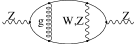
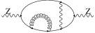
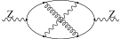
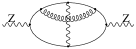
                    (a)  (b)           (c)  (d)

FIG. 2.: QCD corrections to the diagram 1(a)

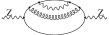
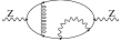
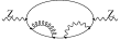
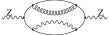
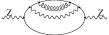
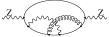
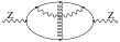
                        (a) (b) (c)               (d) (e) (f)        (g)

FIG. 3.: QCD corrections to the diagram 1(b)

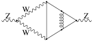
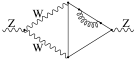
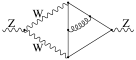
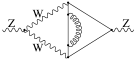
                    (a)  (b)           (c)  (d)

FIG. 4.: QCD corrections to the diagram 1(c)

REFERENCES

[1]
K. Chetyrkin, J. Kühn, and A. Kwiatkowski, CERN Yellow Report 95-03
p. 175, and references therein.
[2]
D. Bardin
et al., CERN Yellow Report 95-03 p. 163, and references therein.
[3]
J. Fleischer, F. Jegerlehner, P. Ra̧czka, and O.V.Tarasov, Phys. Lett.
B293, 437 (1992).
[4]
G. Buchalla and A. Buras, Nucl. Phys. B398, 285 (1993).
[5]
G. Degrassi, Nucl. Phys. B407, 271 (1993).
[6]
K. Chetyrkin, A. Kwiatkowski, and M. Steinhauser, Mod. Phys. Lett. A8,
2785 (1993).
[7]
A. Kwiatkowski and M. Steinhauser, Phys. Lett. B344, 359 (1995).
[8]
S. Peris and A. Santamaria, Nucl. Phys. B445, 252 (1995).
[9]
A. Kataev, Phys. Lett. B287, 209 (1992).
[10]
B. Grzadkowski, J.H. Kühn, P. Krawczyk, and R.G. Stuart,
Nucl. Phys. B281, 18 (1987).
[11]
W. Beenakker and W. Hollik, Z. Phys. C40, 141 (1988).
[12]
S. A. Larin, F. V. Tkachov, and J. Vermaseren,
preprint NIKHEF-H/91-18 (1991) (unpublished).
[13]
J. A. M. Vermaseren, Symbolic manipulation with FORM, CAN, Amsterdam,
1991.
[14]
W. Marciano and D. Wyler, Z. Phys. C3, 181 (1979).
[15]
E. Braaten and A. Kumar, Phys. Rev. D37, 3349 (1988).
[16]
E. W. N. Glover and J. J. van der Bij (conv.),
in G. Altarelli, R. Kleiss, and C. Verzegnassi (eds.),
Z Physics at LEP 1, CERN Yellow Report 89-08.
(a)(b)(c)