MPI-Ph/96-57
TUM-T31-94/96
HD-THEP-96-23
hep-ph/9608365


A 1996 Analysis of the CP Violating Ratio $\varepsilon^{\prime}/\varepsilon$

Abstract

We update our 1993 analysis of the CP violating ratio $\varepsilon^{\prime}/\varepsilon$ in view of the changes in several input parameters, in particular the improved value of the top quark mass. We also investigate the strange quark mass $m_{s}$ dependence of $\varepsilon^{\prime}/\varepsilon$ in view of rather low values found in the most recent lattice calculations. A simple scanning of the input parameters within one standard deviation gives the ranges: $-1.2\cdot 10^{-4}\leq\varepsilon^{\prime}/\varepsilon\leq 16.0\cdot 10^{-4}$ and $0\leq\varepsilon^{\prime}/\varepsilon\leq 43.0\cdot 10^{-4}$ for $m_{\rm s}(m_{\rm c})=150\pm 20~{}\,{\rm MeV}$ and $m_{\rm s}(m_{\rm c})=100\pm 20~{}\,{\rm MeV}$ respectively. If the experimentally measured numbers and the theoretical input parameters are used with Gaussian errors, we find $\varepsilon^{\prime}/\varepsilon=(3.6\pm 3.4)\cdot 10^{-4}$ and $\varepsilon^{\prime}/\varepsilon=(10.4\pm 8.3)\cdot 10^{-4}$ respectively. We also give results for ${\rm Im}V_{ts}^{*}V_{td}$. Analyzing the dependence of $\varepsilon^{\prime}/\varepsilon$ on various parameters we find that only for $m_{\rm s}(m_{\rm c})\leq 100\,\,{\rm MeV}$ and a conspiration of other input parameters, values for $\varepsilon^{\prime}/\varepsilon$ as large as $(2-4)\cdot 10^{-3}$ and consistent with the NA31 result can be obtained.

xxx

The measurement of $\varepsilon^{\prime}/\varepsilon$ at the $10^{-4}$ level remains as one of the important targets of contemporary particle physics. A non-vanishing value of this ratio would give the first signal for the direct CP violation ruling out the superweak models. The experimental situation on Re($\varepsilon^{\prime}/\varepsilon$) is unclear at present. While the result of NA31 collaboration at CERN with Re$(\varepsilon^{\prime}/\varepsilon)=(23\pm 7)\cdot 10^{-4}$ [1] clearly indicates direct CP violation, the value of E731 at Fermilab, Re$(\varepsilon^{\prime}/\varepsilon)=(7.4\pm 5.9)\cdot 10^{-4}$ [2], is compatible with superweak theories [3] in which $\varepsilon^{\prime}/\varepsilon=0$. Hopefully, in about two years the experimental situation concerning $\varepsilon^{\prime}/\varepsilon$ will be clarified through the improved measurements by the two collaborations at the $10^{-4}$ level and by the KLOE experiment at DA$\Phi$NE.

There is no question about that the direct CP violation is present in the standard model. Yet, accidentally it could turn out that it will be difficult to see it in $K\to\pi\pi$ decays. Indeed in the standard model $\varepsilon^{\prime}/\varepsilon$ is governed by QCD penguins and electroweak (EW) penguins. In spite of being suppressed by $\alpha/\alpha_{s}$ relative to QCD penguin contributions, the electroweak penguin contributions have to be included because of the additional enhancement factor ${\rm Re}A_{0}/{\rm Re}A_{2}=22$ relative to QCD penguins. With increasing $m_{\rm t}$ the EW penguins become increasingly important [4, 5], and entering $\varepsilon^{\prime}/\varepsilon$ with the opposite sign to QCD penguins suppress this ratio for large $m_{\rm t}$. For $m_{\rm t}\approx 200\,\,{\rm GeV}$ the ratio can even be zero [5]. Because of this strong cancelation between two dominant contributions and due to uncertainties related to hadronic matrix elements of the relevant local operators, a precise prediction of $\varepsilon^{\prime}/\varepsilon$ is not possible at present.

In spite of all these difficulties, a considerable progress has been made in this decade to calculate $\varepsilon^{\prime}/\varepsilon$. First of all the complete next-to-leading order (NLO) effective hamiltonians for $\Delta S=1$ [6, 7, 8], $\Delta S=2$ [9, 10, 11] and $\Delta B=2$ [9] are now available so that a complete NLO analysis of $\varepsilon^{\prime}/\varepsilon$ including constraints from the observed indirect CP violation ($\varepsilon_{K}$) and the $B^{0}_{d}-\bar{B}^{0}_{d}$ mixing ($\Delta m_{B_{d}}$) is possible. The improved determination of the $V_{ub}$ and $V_{cb}$ elements of the CKM matrix [12, 13], and in particular the determination of the top quark mass $m_{\rm t}$ [14] had of course also an important impact on $\varepsilon^{\prime}/\varepsilon$. The main remaining theoretical uncertainties in this ratio are then the poorly known hadronic matrix elements of the relevant QCD penguin and electroweak penguin operators, the values of the non-perturbative parameters $B_{K}$ and $\sqrt{B_{B}}F_{B}$ and as stressed in [7] the values of $m_{\rm s}$ and $\Lambda_{\overline{MS}}$.

In 1993 we have presented a detailed NLO analysis of $\varepsilon^{\prime}/\varepsilon$ [7] using all information available at that time. A similar NLO analysis has been made by the Rome group [15]. In 1995 the latter group has updated their analysis to predict a very small ratio $\varepsilon^{\prime}/\varepsilon=(3.1\pm 2.5)\cdot 10^{-4}$ [16], essentially consistent with the superweak scenario. An analysis of $\varepsilon^{\prime}/\varepsilon$ with different treatments of hadronic matrix elements can be found in [17, 18, 19] and will be briefly discussed below.

The purpose of the present letter is to update our 1993 analysis and to confront our new result with the one of the Rome group [16] and with [17, 18, 19].

Let us list the main new ingredients of our present analysis compared to the previous one:

• The value of the top quark mass from CDF and D0 [14],

• Updated values for the elements of the CKM matrix such as $V_{ub}$ and $V_{cb}$ [12, 13],

• New values of the strange quark mass ($m_{\rm s}$) coming from most recent lattice [20, 21, 22] and QCD sum rule [23, 24, 25] calculations,

• Improved value for $\alpha_{s}(M_{Z})$ [26], for which we take $\alpha_{s}(M_{Z})=0.118\pm 0.005$ corresponding to $\Lambda_{\overline{\rm MS}}^{(4)}=325\pm 80\,{\rm MeV}$,

• The inclusion of NLO corrections to the QCD factor $\eta_{3}$ [11] entering the top-charm contribution in the $\Delta S=2$ effective hamiltonian, the last previously missing ingredient of a complete NLO analysis of $\varepsilon^{\prime}/\varepsilon$, and

• Two distinct analyses of theoretical and experimental uncertainties.

Let us first recall the basic formulae used in our new analysis, referring frequently to our 1993 paper [7] where further details can be found. In [7] we have analyzed $\varepsilon^{\prime}/\varepsilon$ in the Standard Model including leading and next-to-leading logarithmic contributions to the Wilson coefficient functions of the relevant local operators [6, 7, 8]. Imposing the constraints from the $CP$ conserving $K\rightarrow\pi\pi$ data on the hadronic matrix elements of these operators we have given numerical results for $\varepsilon^{\prime}/\varepsilon$ as a function of $\Lambda_{\overline{\rm MS}}$, $m_{\rm t}$, $m_{\rm s}$ and two non-perturbative parameters $B_{6}^{(1/2)}$ and $B_{8}^{(3/2)}$ which cannot be fixed by the $CP$ conserving data at present. These two parameters are defined by

$$\langle Q_{6}(m_{\rm c})\rangle_{0}\equiv B_{6}^{(1/2)}\,\langle Q_{6}(m_{\rm c})\rangle_{0}^{\rm(vac)}\qquad\langle Q_{8}(m_{\rm c})\rangle_{2}\equiv B_{8}^{(3/2)}\,\langle Q_{8}(m_{\rm c})\rangle_{2}^{\rm(vac)}\,,$$ (1)

where

$$Q_{6}=\left(\bar{s}_{\alpha}\,d_{\beta}\right)_{\rm V-A}\sum_{q}\left(\bar{q}_{\beta}\,q_{\alpha}\right)_{\rm V+A}\qquad Q_{8}=\frac{3}{2}\left(\bar{s}_{\alpha}\,d_{\beta}\right)_{\rm V-A}\sum_{q}e_{q}\left(\bar{q}_{\beta}\,q_{\alpha}\right)_{\rm V+A}$$ (2)

are the dominant QCD and electroweak penguin operators, respectively. The subscripts on the hadronic matrix elements denote the isospin of the final $\pi\pi$-state. The label “vac” stands for the vacuum insertion estimate of the hadronic matrix elements in question for which $B_{6}^{(1/2)}=B_{8}^{(3/2)}=1$. The same result is found in the large $N$ limit [27, 28]. Also lattice calculations give similar results $B_{6}^{(1/2)}=1.0\pm 0.2$ [29, 30] and $B_{8}^{(3/2)}=1.0\pm 0.2$ [29, 30, 31, 32], $B_{8}^{(3/2)}=0.81(1)$ [33]. We have demonstrated in [7] that in QCD the parameters $B_{6}^{(1/2)}$ and $B_{8}^{(3/2)}$ depend only very weakly on the renormalization scale $\mu$ when $\mu>1\,{\rm GeV}$ is considered. The $\mu$ dependence for the matrix elements in (1) is then given to an excellent accuracy by $1/m_{\rm s}^{2}(\mu)$ with $m_{\rm s}(\mu)$ denoting the running strange quark mass. The scale $\mu=m_{\rm c}$ in (1) is a convenient choice for the extraction of matrix elements from the CP conserving data.

At this point it seems appropriate to summarize the present status of the value of the strange quark mass. The most recent results of QCD sum rule (QCDSR) calculations [23, 24, 25] obtained at $\mu=1~{}GeV$ correspond to $m_{\rm s}(m_{\rm c})=170\pm 20\,\,{\rm MeV}$ with $m_{\rm c}=1.3\,\,{\rm GeV}$. The lattice calculation of [20] finds $m_{\rm s}(2\,\,{\rm GeV})=128\pm 18\,\,{\rm MeV}$ which corresponds to $m_{\rm s}(m_{\rm c})=150\pm 20\,\,{\rm MeV}$, in rather good agreement with the QCDSR result. This summer a new lattice result has been presented by Gupta and Bhattacharya [21]. In the quenched approximation they find $m_{\rm s}(2\,\,{\rm GeV})=90\pm 20\,\,{\rm MeV}$ corresponding to $m_{\rm s}(m_{\rm c})=105\pm 20\,\,{\rm MeV}$. For $n_{f}=2$ the value is found to be even lower: $m_{\rm s}(2\,\,{\rm GeV})=70\pm 15\,\,{\rm MeV}$ corresponding to $m_{\rm s}(m_{\rm c})=82\pm 17\,\,{\rm MeV}$. Similar results are expected to come soon from the lattice group at FNAL[22]. Certainly these results are on the low side of all strange quark mass determinations.

Now, as an average from quenched lattice QCD, we can take $m_{\rm s}(m_{\rm c})=130\pm 20\,\,{\rm MeV}$ and when averaged with the QCD sum rule value, we arrive at $m_{\rm s}(m_{\rm c})=150\pm 20\,\,{\rm MeV}$. This will be one of the ranges for the strange quark mass to be used in our analysis. On the other hand we cannot exclude at present that the ultimate values for $m_{\rm s}$ will be as low as found in the most recent lattice calculations [21, 22]. In order to cover this possibility we will also present results for $m_{\rm s}(m_{\rm c})=100\pm 20\,\,{\rm MeV}$. In table 1 we provide the dictionary between the values of $m_{\rm s}$ normalized at different scales. To this end we have used the standard renormalization group formula at two-loop level with $\Lambda_{\overline{\rm MS}}^{(4)}=325~{}\,{\rm MeV}$.

Table 1: The dictionary between the values of $m_{\rm s}$ in units of $\,{\rm MeV}$ normalized at different scales with $m_{\rm c}=1.3~{}\,{\rm GeV}$.

$m_{\rm s}(m_{\rm c})$	$~{}75$	$100$	$125$	$150$	$175$
$m_{\rm s}(2~{}\,{\rm GeV})$	$~{}65$	$~{}86$	$108$	$129$	$151$
$m_{\rm s}(1~{}\,{\rm GeV})$	$~{}87$	$116$	$144$	$173$	$202$

It should also be remarked that the decomposition of the relevant hadronic matrix elements of penguin operators into a product of $B_{i}$ factors times $1/m_{s}^{2}$ although useful in the $1/N$ approach is unnecessary in a brute force method like the lattice approach. It is to be expected that the future lattice calculations will directly give the relevant hadronic matrix elements and the issue of $m_{\rm s}$ in connection with $\varepsilon^{\prime}/\varepsilon$ will effectively disappear.

The details of the calculation of the Wilson coefficient functions as well as the determination of the hadronic matrix elements from the CP-conserving data can be found in [7] and will not be repeated here. We will rather present an update of the analytic formula for $\varepsilon^{\prime}/\varepsilon$ of ref. [34] which to a very good accuracy represents our numerical analysis. This analytic formula exhibits the dependence of $\varepsilon^{\prime}/\varepsilon$ on $m_{\rm t}$, $m_{\rm s}$, $\Lambda_{\overline{\rm MS}}^{(4)}$, $B_{6}^{(1/2)}$ and $B_{8}^{(3/2)}$. It is given as follows:

$$\varepsilon^{\prime}/\varepsilon={\rm Im}\lambda_{t}\,F(x_{t})\,,$$ (3)

where

$$F(x_{t})=P_{0}+P_{X}\,X_{0}(x_{t})+P_{Y}\,Y_{0}(x_{t})+P_{Z}\,Z_{0}(x_{t})+P_{E}\,E_{0}(x_{t})\,,$$ (4)

and

$${\rm Im}\lambda_{t}={\rm Im}V_{ts}^{*}V_{td}=|V_{\rm ub}|\,|V_{\rm cb}|\,\sin\delta=\eta\,\lambda^{5}\,A^{2}$$ (5)

in the standard parameterization of the CKM matrix [35] and in the Wolfenstein parameterization [36], respectively.

The $m_{\rm t}$-dependent functions in (4) are given by

$$X_{0}(x_{t}) = \frac{x_{t}}{8}\,\left[\frac{x_{t}+2}{x_{t}-1}+\frac{3x_{t}-6}{(x_{t}-1)^{2}}\ln x_{t}\right]$$

$$Y_{0}(x_{t}) = \frac{x_{t}}{8}\,\left[\frac{x_{t}-4}{x_{t}-1}+\frac{3x_{t}}{(x_{t}-1)^{2}}\ln x_{t}\right]$$ (6)

$$Z_{0}(x_{t}) = -\frac{1}{9}\ln x_{t}+\frac{18x_{t}^{4}-163x_{t}^{3}+259x_{t}^{2}-108x_{t}}{144(x_{t}-1)^{3}}+$$

$$\frac{32x_{t}^{4}-38x_{t}^{3}-15x_{t}^{2}+18x_{t}}{72(x_{t}-1)^{4}}\ln x_{t}$$

$$E_{0}(x_{t}) = -\frac{2}{3}\ln x_{t}+\frac{x_{t}^{2}(15-16x_{t}+4x_{t}^{2})}{6(1-x_{t})^{4}}\ln x_{t}+\frac{x_{t}(18-11x_{t}-x_{t}^{2})}{12(1-x_{t})^{3}}$$

with $x_{t}=m_{\rm t}^{2}/M_{\rm W}^{2}$. In the range $150\,{\rm GeV}\leq m_{\rm t}\leq 200\,{\rm GeV}$ these functions can be approximated to better than 1% accuracy by the following expressions [37]

$$X_{0}(x_{t})=0.660\,x_{t}^{0.575} Y_{0}(x_{t})=0.315\,x_{t}^{0.78}$$ (7)

$$Z_{0}(x_{t})=0.175\,x_{t}^{0.93} E_{0}(x_{t})=0.564\,x_{t}^{-0.51}\,.$$

The coefficients $P_{i}$ are given in terms of $B_{6}^{(1/2)}\equiv B_{6}^{(1/2)}(m_{\rm c})$, $B_{8}^{(3/2)}\equiv B_{8}^{(3/2)}(m_{\rm c})$ and $m_{\rm s}(m_{\rm c})$ as follows

$$P_{i}=r_{i}^{(0)}+\left[\frac{158\,{\rm MeV}}{m_{\rm s}(m_{\rm c})+m_{\rm d}(m_{\rm c})}\right]^{2}\left(r_{i}^{(6)}B_{6}^{(1/2)}+r_{i}^{(8)}B_{8}^{(3/2)}\right)\,.$$ (8)

The $P_{i}$ are renormalization scale and scheme independent. They depend however on $\Lambda_{\overline{\rm MS}}$. In table 2 we give the numerical values of $r_{i}^{(0)}$, $r_{i}^{(6)}$ and $r_{i}^{(8)}$ for different values of $\Lambda_{\overline{\rm MS}}^{(4)}$ at $\mu=m_{\rm c}$ in the NDR renormalization scheme. The coefficients $r_{i}^{(0)}$, $r_{i}^{(6)}$ and $r_{i}^{(8)}$ depend only very weakly on $m_{\rm s}(m_{\rm c})$ as the dominant $m_{\rm s}$ dependence has been factored out. The numbers given in table 2 correspond to $m_{\rm s}(m_{\rm c})=150\,\,{\rm MeV}$. However, even for $m_{\rm s}(m_{\rm c})\approx 100\,{\rm MeV}$ the analytic expressions given here reproduce our numerical calculations of $\varepsilon^{\prime}/\varepsilon$ to better than $4\%$. For different scales $\mu$ the numerical values in the tables change without modifying the values of the $P_{i}$’s as it should be. To this end also $B_{6}^{(1/2)}$ and $B_{8}^{(3/2)}$ have to be modified as they depend albeit weakly on $\mu$.

Concerning the scheme dependence only the $r_{0}$ coefficients are scheme dependent at the NLO level. Their values in the HV scheme are given in the last row of table 2. The coefficients $r_{i}$, $i=X,Y,Z,E$ are on the other hand scheme independent at NLO. This is related to the fact that the $m_{\rm t}$ dependence in $\varepsilon^{\prime}/\varepsilon$ enters first at the NLO level and consequently all coefficients $r_{i}$ in front of the $m_{\rm t}$ dependent functions must be scheme independent.

Consequently, when changing the renormalization scheme one is only obliged to change appropriately $B_{6}^{(1/2)}$ and $B_{8}^{(3/2)}$ in the formula for $P_{0}$ in order to obtain a scheme independence of $\varepsilon^{\prime}/\varepsilon$. In calculating $P_{i}$ where $i\not=0$, $B_{6}^{(1/2)}$ and $B_{8}^{(3/2)}$ can in fact remain unchanged, because their variation in this part corresponds to higher order contributions to $\varepsilon^{\prime}/\varepsilon$ which would have to be taken into account in the next order of perturbation theory.

For similar reasons the NLO analysis of $\varepsilon^{\prime}/\varepsilon$ is still insensitive to the precise definition of $m_{\rm t}$. In view of the fact that the NLO calculations needed to extract ${\rm Im}\lambda_{t}$ (see below) have been done with $m_{\rm t}=\overline{m}_{t}(m_{\rm t})$ we will also use this definition in calculating $F(x_{t})$. The value for $\overline{m}_{t}(m_{\rm t})$ corresponding to the average pole mass $m_{\rm t}^{pole}=175\pm 6\,\,{\rm GeV}$ from CDF and D0 [14], is $\overline{m_{\rm t}}(m_{\rm t})=167\pm 6\,{\rm GeV}$. In what follows $m_{\rm t}$ stands always for $\overline{m}_{t}(m_{\rm t})$.

Table 2: $\Delta S=1$ PBE coefficients for various $\Lambda_{\overline{\rm MS}}$ in the NDR scheme. The last row gives the $r_{0}$ coefficients in the HV scheme.

	$\Lambda_{\overline{\rm MS}}^{(4)}=245\,{\rm MeV}$			$\Lambda_{\overline{\rm MS}}^{(4)}=325\,{\rm MeV}$			$\Lambda_{\overline{\rm MS}}^{(4)}=405\,{\rm MeV}$
$i$	$r_{i}^{(0)}$	$r_{i}^{(6)}$	$r_{i}^{(8)}$	$r_{i}^{(0)}$	$r_{i}^{(6)}$	$r_{i}^{(8)}$	$r_{i}^{(0)}$	$r_{i}^{(6)}$	$r_{i}^{(8)}$
0	–2.674	6.537	1.111	–2.747	8.043	0.933	–2.814	9.929	0.710
$X$	0.541	0.011	0	0.517	0.015	0	0.498	0.019	0
$Y$	0.408	0.049	0	0.383	0.058	0	0.361	0.068	0
$Z$	0.178	–0.009	–6.468	0.244	–0.011	–7.402	0.320	–0.013	–8.525
$E$	0.197	–0.790	0.278	0.176	–0.917	0.335	0.154	–1.063	0.402
0	–2.658	5.818	0.839	–2.729	6.998	0.639	–2.795	8.415	0.398

The inspection of the table 2 shows that the terms involving $r_{0}^{(6)}$ and $r_{Z}^{(8)}$ dominate the ratio $\varepsilon^{\prime}/\varepsilon$. The function $Z_{0}(x_{t})$ representing a gauge invariant combination of $Z^{0}$- and $\gamma$-penguins grows rapidly with $m_{\rm t}$ and due to $r_{Z}^{(8)}<0$ these contributions suppress $\varepsilon^{\prime}/\varepsilon$ strongly for large $m_{\rm t}$ [4, 5].

In order to complete our analysis of $\varepsilon^{\prime}/\varepsilon$ we need the value of ${\rm Im}\lambda_{t}$. To this end we will use the standard expression for $\varepsilon_{K}$ describing the indirect CP violation in $K\to\pi\pi$ and the corresponding expression for $\Delta m_{B_{d}}$ which describes the $B^{0}_{d}$-$\bar{B}^{0}_{d}$ mixing. Since these expressions are by now well known we will not repeat them here. They can be found in [37]. We list here only the QCD factors $\eta_{i}\,(i=1,2,3)$ and $\eta_{B}$ relevant for $\varepsilon_{K}$ and $x_{d}$ respectively:

$$\eta_{1}=1.38\qquad\eta_{2}=0.57\qquad\eta_{3}=0.47\qquad\eta_{B}=0.55$$ (9)

They all include NLO corrections [9, 10, 11].

The resulting value for ${\rm Im}\lambda_{t}$ depends on several input parameters such as $|V_{cb}|$, $|V_{ub}/V_{cb}|$, $m_{\rm t}$, $B_{K}$ and $\sqrt{B_{B_{d}}}F_{B_{d}}$. Here $B_{i}$ are the non-perturbative parameters related to the hadronic matrix elements of the $\Delta S=2$ and $\Delta B=2$ operators and $F_{B_{d}}$ is the $B_{d}$ meson decay constant. Values and errors of these input parameters, used in the present analysis, are collected in table 3 together with the experimental values for $\varepsilon_{K}$ [35] and $\Delta m_{B_{d}}$ [13]. Except for $m_{\rm t}$, $\varepsilon_{K}$, $\Delta m_{B_{d}}$ and $\Lambda_{\overline{\rm MS}}^{(4)}$ all input quantities are the same as in the review [37] where further details on the chosen ranges with relevant references can be found. See also [38]. For $\tau(B_{d})=1.6~{}ps$ the value for $\Delta m_{B_{d}}$ in table 3 corresponds to the mixing parameter $x_{d}=0.74\pm 0.03$

Table 3: Collection of input parameters.

Quantity	Central	Error
$|V_{cb}|$	0.040	$\pm 0.003$
$|V_{ub}/V_{cb}|$	0.080	$\pm 0.020$
$B_{K}$	0.75	$\pm 0.15$
$\sqrt{B_{d}}F_{B_{d}}$	$200\,{\rm MeV}$	$\pm 40\,{\rm MeV}$
$\Lambda_{\overline{\rm MS}}^{(4)}$	$325\,{\rm MeV}$	$\pm 80\,{\rm MeV}$
$m_{\rm t}$	$167\,{\rm GeV}$	$\pm 6\,{\rm GeV}$
$\Delta m_{B_{d}}$	$0.464~{}ps^{-1}$	$\pm 0.018~{}ps^{-1}$
$\varepsilon_{K}$	$2.280\cdot 10^{-3}$	$\pm 0.013\cdot 10^{-3}$

In what follows we will present two types of the numerical analyses of ${\rm Im}\lambda_{t}$ and $\varepsilon^{\prime}/\varepsilon$:

• Method 1: Both the experimentally measured numbers and the theoretical input parameters are scanned independently within the errors given in table 3.

• Method 2: The experimentally measured numbers and the theoretical input parameters are used with Gaussian errors.

Figure 1: Probability density distribution for ${\rm Im}\lambda_{t}$ using input parameters as given in the text.

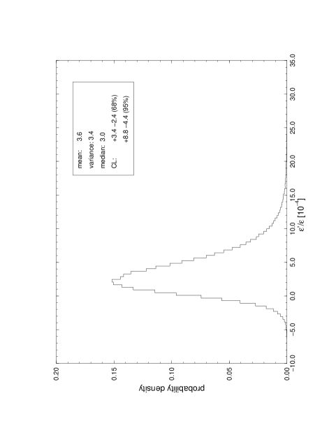
Figure 2: Probability density distribution for $\varepsilon^{\prime}/\varepsilon$ for $m_{\rm s}(m_{\rm c})=150\pm 20\,\,{\rm MeV}$ using other input parameters as given in the text.

The first method is the one used in our 1993 paper as well as in [37]. The second method is similar to the one used by the Rome group [16] except that these authors assume a flat distribution (with a width of $2\sigma$) for the theoretical quantities. Whereas the first method is even more conservative than adding all errors for the various input parameters linearly, the second method yields a similar error estimate as if all errors would have been added in quadrature. Thus the second method should be considered as reflecting a lower bound on the combined error with the true uncertainty lying somewhere in between the two methods.

In our new analysis let us first concentrate on the case $m_{\rm s}(m_{\rm c})=150\pm 20\,\,{\rm MeV}$. Using the first method and the parameters in table 3 we find :

$$0.86\cdot 10^{-4}\leq{\rm Im}\lambda_{t}\leq 1.71\cdot 10^{-4}$$ (10)

$$-1.2\cdot 10^{-4}\leq\varepsilon^{\prime}/\varepsilon\leq 16.0\cdot 10^{-4}$$ (11)

These ranges are similar to the ones found in [37] where slightly larger errors for $m_{t}$ and $\Delta m_{B_{d}}$ have been used.

Using next the second method we find the distributions of values for ${\rm Im}\lambda_{t}$ and $\varepsilon^{\prime}/\varepsilon$ in figs. 1 and 2, respectively. From the distributions in figs. 1 and 2 we deduce the following results:

$${\rm Im}\lambda_{t}=(1.29\pm 0.22)\cdot 10^{-4}$$ (12)

$$\varepsilon^{\prime}/\varepsilon=(3.6\pm 3.4)\cdot 10^{-4}$$ (13)

In addition in the figures we have also given central values according to the median prescription and the corresponding 1 and $2\,\sigma$ confidence intervals. Within the errors, they agree with mean and variance. We observe that the distribution of the values of $\varepsilon^{\prime}/\varepsilon$ is asymmetric with a longer tail towards larger values. However at $95\%$ C.L. small negative values cannot be excluded.

The above results for $\varepsilon^{\prime}/\varepsilon$ apply to the NDR scheme. $\varepsilon^{\prime}/\varepsilon$ is generally lower in the HV scheme if the same values for $B_{6}^{(1/2)}$ and $B_{8}^{(3/2)}$ are used in both schemes. In view of the fact that the differences between NDR and HV schemes are smaller than the uncertainties in $B_{6}^{(1/2)}$ and $B_{8}^{(3/2)}$ we think it is sufficient to present only the results in the NDR scheme here. The results in the HV scheme can be found in [7, 16].

In spite of some differences in the treatment of hadronic matrix elements our results for $\varepsilon^{\prime}/\varepsilon$, with $m_{\rm s}(m_{\rm c})=150\pm 20\,{\rm MeV}$, using the second method agree well with the results of the Rome group [16]. On the other hand the range in (11) shows that for particular choices of the input parameters, values for $\varepsilon^{\prime}/\varepsilon$ as high as $15\cdot 10^{-4}$ cannot be excluded at present. Such high values are found if simultaneously $|V_{ub}/V_{cb}|=0.10$, $B_{6}=1.2$, $B_{8}=0.8$, $B_{K}=0.6$, $m_{\rm s}(m_{\rm c})=130MeV$, $\Lambda_{\overline{\rm MS}}^{(4)}=405\,{\rm MeV}$ and low values of $m_{t}$ still consistent with $\varepsilon_{K}$ and the observed $B^{0}_{d}-\bar{B}^{0}_{d}$ mixing are chosen. It is however evident from figure 2 that such high values of $\varepsilon^{\prime}/\varepsilon$ and generally values above $10^{-3}$ are very improbable.

In [18] the hadronic matrix elements relevant for $\varepsilon^{\prime}/\varepsilon$ have been calculated within the chiral quark model. Using the first method the authors find a rather large range $-50\cdot 10^{-4}\leq\varepsilon^{\prime}/\varepsilon\leq 14\cdot 10^{-4}$. In particular they find in contrast to [7, 16, 37] and the present analysis that negative values for $\varepsilon^{\prime}/\varepsilon$ as large as $-5\cdot 10^{-3}$ are possible. This is related to the fact that in the chiral quark model $B_{6}$ and $B_{8}$ can for certain model parameters deviate considerably from unity and generally $B_{8}>B_{6}$. The Dortmund group [17] advocates on the other hand $B_{6}>B_{8}$ to find $\varepsilon^{\prime}/\varepsilon=(9.9\pm 4.1)\cdot 10^{-4}$ for $m_{\rm s}(1\,{\rm GeV})=175\,\,{\rm MeV}$ [19]. From the point of view of the present analysis and the results of the Rome group such high values of $\varepsilon^{\prime}/\varepsilon$ for $m_{\rm s}(m_{\rm c})={\cal O}(150\,\,{\rm MeV})$ are rather improbable within the standard model.

Figure 3: Probability density distribution for $\varepsilon^{\prime}/\varepsilon$ for $m_{\rm s}(m_{\rm c})=100\pm 20\,\,{\rm MeV}$ using other input parameters as given in the text.

The situation with $\varepsilon^{\prime}/\varepsilon$ in the standard model may however change considerably if the value for $m_{\rm s}$ is as low as found in [21, 22]. Repeating our analysis for $m_{\rm s}(m_{\rm c})=100\pm 20\,\,{\rm MeV}$ we find

$$0\leq\varepsilon^{\prime}/\varepsilon\leq 43.0\cdot 10^{-4}$$ (14)

and

$$\varepsilon^{\prime}/\varepsilon=(10.4\pm 8.3)\cdot 10^{-4}$$ (15)

in place of (11) and (13) respectively. The corresponding distribution is shown in fig. 3. We observe that the resulting distribution of the values of $\varepsilon^{\prime}/\varepsilon$ is in this case rather asymmetric with a very long tail towards substantial positive values. Moreover, negative values of $\varepsilon^{\prime}/\varepsilon$ are found to be very unlikely.

In addition, it is of interest to investigate for which values of the input parameters the standard model can reproduce the results of NA31 and E731 collaborations. In table 4 we present the values of $\varepsilon^{\prime}/\varepsilon$ for five choices of $m_{\rm s}(m_{\rm c})$ and for selective sets of other input parameters keeping $V_{cb}=0.040$, $m_{\rm t}=167\,\,{\rm GeV}$ and $B_{K}=0.75$ fixed. The values of $\varepsilon^{\prime}/\varepsilon$ given in this table correspond to $\sin\delta$ in the first quadrant. The results for the second quadrant turn out to be somewhat lower. We observe that the decrease of $m_{\rm s}$ for $m_{\rm s}(m_{\rm c})\geq 100\,{\rm MeV}$ alone is insufficient to bring the standard model to agree with the values obtained by the NA31 collaboration. For central values of other parameters and $m_{\rm s}(m_{\rm c})={\cal O}(100\,\,{\rm MeV})$ the standard model prediction is rather in the ball park of the E731 result. However for $B_{6}>B_{8}$, sufficiently large values of $|V_{ub}/V_{cb}|$ and $\Lambda_{\overline{\rm MS}}$ and small values of $m_{\rm s}(m_{\rm c})$, the values of $\varepsilon^{\prime}/\varepsilon$ in the standard model can be as large as $(2-4)\cdot 10^{-3}$ and consistent with the NA31 result.

Table 4: Values of $\varepsilon^{\prime}/\varepsilon$ in units of $10^{-4}$ for specific values of various input parameters at $m_{\rm t}=167\,\,{\rm GeV}$, $V_{cb}=0.040$ and $B_{K}=0.75$.

$|V_{ub}/V_{cb}|$	$\Lambda_{\overline{\rm MS}}^{(4)}\;[\,{\rm MeV}]$	$B_{6}$	$B_{8}$	$m_{\rm s}(m_{\rm c})\,[\,{\rm MeV}]$	$\varepsilon^{\prime}/\varepsilon$
				$~{}75$	$16.8$
				$100$	$~{}9.1$
$0.08$	$325$	$1.0$	$1.0$	$125$	$~{}5.3$
				$150$	$~{}3.2$
				$175$	$~{}1.8$
				$~{}75$	$27.8$
				$100$	$15.6$
$0.08$	$325$	$1.2$	$0.8$	$125$	$~{}9.6$
				$150$	$~{}6.2$
				$175$	$~{}4.1$
				$~{}75$	$39.8$
				$100$	$22.5$
$0.10$	$405$	$1.2$	$0.8$	$125$	$14.0$
				$150$	$~{}9.2$
				$175$	$~{}6.2$

To summarize, we have presented a new analysis of $\varepsilon^{\prime}/\varepsilon$, showing in particular the dependence of this important ratio on various input parameters, in particular the value of $m_{\rm s}$. Our results are summarized in (11) and (13) for the case $m_{\rm s}(m_{\rm c})=150\pm 20\,\,{\rm MeV}$ and in (14) and (15) for the case $m_{\rm s}(m_{\rm c})=100\pm 20\,\,{\rm MeV}$. Furthermore, table 4 gives values of $\varepsilon^{\prime}/\varepsilon$ for particular sets of input parameters. The improved results for ${\rm Im}\lambda_{t}$ are given in (10) and (12).

It is clear that the fate of $\varepsilon^{\prime}/\varepsilon$ in the standard model after the improved measurement of $m_{\rm t}$, depends sensitively on the values of $|V_{ub}/V_{cb}|$, $\Lambda_{\overline{\rm MS}}$ and in particular on $B_{6}$, $B_{8}$ and $m_{\rm s}$. For $m_{\rm s}(m_{\rm c})={\cal O}(150\,\,{\rm MeV})$ $\varepsilon^{\prime}/\varepsilon$ is generally below $10^{-3}$ in agreement with E731 with central values in the ball park of a few $10^{-4}$ as found in [16, 37] and here. However, if the low values of $m_{\rm s}(m_{\rm c})={\cal O}(100\,\,{\rm MeV})$ found in [21, 22] are confirmed by other groups in the future, a conspiration of other parameters may give values as large as $(2-4)\cdot 10^{-3}$ in the ball park of the NA31 result.

Let us hope that the future experimental and theoretical results will be sufficiently accurate to be able to see whether $\varepsilon^{\prime}/\varepsilon\not=0$ and whether the standard model agrees with the data. In any case the coming years should be very exciting.

References

[1]G. D. Barret al.,
Phys. Lett.B317 (1993) 233.
[2]L. K. Gibbonset al.,
Phys. Rev. Lett.70 (1993) 1203.
[3]L. Wolfenstein,
Phys. Rev. Lett.13 (1964) 562.
[4]J. M. Flynn and L. Randall,
Phys. Lett.B224 (1989) 221; erratum ibid. Phys.
Lett.B235 (1990) 412.
[5]G. Buchalla, A. J. Buras, and M. K. Harlander,
Nucl. Phys.B337 (1990) 313.
[6]A. J. Buras, M. Jamin, M. E. Lautenbacher, and P. H.
Weisz,
Nucl. Phys.B370 (1992) 69; addendum ibid. Nucl. Phys.B375 (1992) 501.
[7]A. J. Buras, M. Jamin, and M. E. Lautenbacher,
Nucl. Phys.B408 (1993) 209.
[8]M. Ciuchini, E. Franco, G. Martinelli, and L. Reina,
Nucl. Phys.B415 (1994) 403.
[9]A. J. Buras, M. Jamin, and P. H. Weisz,
Nucl. Phys.B347 (1990) 491.
[10]S. Herrlich and U. Nierste,
Nucl. Phys.B419 (1994) 292.
[11]S. Herrlich and U. Nierste,
Phys. Rev.D52 (1995) 6505.
[12]M. Neubert,
invited talked presented at the 27th Lepton-Photon Symposium,
Beijing, China (August 1995), CERN preprint,CERN-TH/95-307;
hep-ph/9511409.
[13]L. Gibbons, Planary talk given at the 28th International Conference
on High Energy Physics, July 1996, Warsaw, Poland.
[14]P. Tipton, Planary talk given at the 28th International Conference
on High Energy Physics, July 1996, Warsaw, Poland.
[15]M. Ciuchini, E. Franco, G. Martinelli, and L. Reina,
Phys. Lett.B301 (1993) 263.
[16]M. Ciuchini, E. Franco, G. Martinelli, L. Reina, and
L. Silvestrini,
Z. Phys.C68 (1995) 239.
[17]J. Heinrich, E. A. Paschos, J.-M. Schwarz, and Y. L.
Wu,
Phys. Lett.B279 (1992) 140.
[18]S. Bertolini, J. O. Eeg, and M. Fabrichesi,
SISSA preprint,SISSA 103/95/EP (1995).
[19]E. A. Paschos,
invited talked presented at the 27th Lepton-Photon Symposium,
Beijing, China (August 1995), University of Dortmund preprint,DO-TH 96/01.
[20]C. R. Allton, M. Ciuchini, M. Crisafulli, V. Lubicz,
and G. Martinelli,
Nucl. Phys.B431 (1994) 667.
[21]R. Gupta and T. Bhattacharya, hep-lat/9605039.
[22]B.J. Gough, G. Hockney, A.X. El-Khadra, A.S. Kronfeld, P.B. Mackenzie,
B. Mertens, T. Onogi and J. Simone, in preparation.
[23]M. Jamin and M. Münz,
Z. Phys.C66 (1995) 633.
[24]K. G. Chetyrkin, C. A. Dominguez, D. Pirjol, and K. Schilcher,
Phys. Rev.D51 (1995) 5090.
[25]S. Narison,
Phys. Lett.B358 (1995) 113.
[26]M. Schmelling, Planary talk given at the 28th International Conference
on High Energy Physics, July 1996, Warsaw, Poland.
[27]W. A. Bardeen, A. J. Buras and J.-M. Gérard,
Phys. Lett.B180 (1986) 133.
[28]A. J. Buras and J.-M. Gérard,
Phys. Lett.B192 (1987) 156.
[29]G. W. Kilcup,
Nucl. Phys.B (Proc. Suppl.) 20 (1991) 417.
[30]S. R. Sharpe,
Nucl. Phys.B (Proc. Suppl.) 20 (1991) 429.
[31]C. Bernard and A. Soni,
Nucl. Phys.B (Proc. Suppl.) 9 (1989) 155.
[32]E. Franco, L. Maiani, G. Martinelli, and A. Morelli,
Nucl. Phys.B317 (1989) 63.
[33]R. Gupta,
talk given at Lattice-96.
[34]A. J. Buras and M. E. Lautenbacher,
Phys. Lett.B318 (1993) 212.
[35]Particle Data Group,
Review of Particle Physics,
Phys. Rev.D54 (1996) 1.
[37]G. Buchalla, A. J. Buras, and M. E. Lautenbacher,
Munich Technical University preprint (to appear in Rev.
Mod. Phys.),TUM-T31-100/95; hep-ph/9512380.
[38]J. Flynn, Planary talk given at the 28th International Conference
on High Energy Physics, July 1996, Warsaw, Poland.