Abstract

We construct a chiral Lagrangian containing besides the usual pion field ($\pi$) also its first radial excitation ($\pi^{\prime}$). The Lagrangian is derived by bosonization of a Nambu–Jona-Lasinio quark model with separable non-local interactions, with form factors corresponding to 3–dimensional ground and excited state wave functions. Chiral symmetry breaking is governed by the NJL gap equation. The effective Lagrangian for $\pi$– and $\pi^{\prime}$–mesons shows the decoupling of the Goldstone pion and the vanishing of the $\pi^{\prime}$ leptonic decay constant, $f_{\pi^{\prime}}$, in the chiral limit, as required by axial current conservation. We derive the excited states’ contribution to the axial current of the model using Noether’s theorem. For finite pion mass and $\pi^{\prime}$ masses in the range of $750\,{\rm MeV}$–$1300\,{\rm MeV}$, $f_{\pi^{\prime}}/f_{\pi}$ is found to be of the order of 1% .

PACS: 12.39.Fe, 12.39.Ki, 11.40.Ha, 14.40.Cs
Keywords: chiral Lagrangians, radial excitations of mesons, chiral quark models  
¹ E-mail: volkov@thsun1.jinr.dubna.su
² E-mail: weiss@hadron.tp2.ruhr-uni-bochum.de

1 Introduction

Radial excitations of light mesons are currently a topic of great interest in hadronic physics. During the next years, facilities at CEBAF and IHEP (Protvino) will provide improved experimental information about excited states in the few–GeV region, e.g. on the $\pi^{\prime}$ meson. The resonance usually identified as the first radial excitation of the pion has a mass of $(1300\pm 100)\,{\rm MeV}$ [1]. Recently, indications of a light resonance in diffractive production of $3\pi$–states have lead to speculations that the mass of the $\pi^{\prime}$ may be considerably lower at $\sim 750\,{\rm MeV}$ [2].

A theoretical description of radially excited pions poses some interesting challenges. The physics of normal pions is completely governed by the spontaneous breaking of chiral symmetry. A convenient way to derive the properties of soft pions is by way of an effective Lagrangian based on a non-linear realization of chiral symmetry [3]. When attempting to introduce higher resonances to extend the effective Lagrangian description to higher energies, one must ensure that the introduction of new degrees of freedom does not spoil the low–energy theorems for pions, which are universal consequences of chiral symmetry. In the case of vector resonances ($\rho,\omega,A_{1}$) this problem can be solved by introducing them as gauge bosons. Such “gauged” chiral Lagrangians have proven very successful in describing meson phenomenology up to $\sim 1\,{\rm GeV}$ [4]. When trying to include $0^{-}$–resonances as elementary fields, however, there is no simple principle to restrict the form of interactions — the $\pi^{\prime}$ has the same spin–parity quantum numbers as the normal pion itself. Nevertheless, the normal pion field must decouple from the “hard” degrees of freedom in the chiral limit in order to describe a Goldstone boson. At the same time, the $\pi^{\prime}$ contributes to the axial vector hadronic current, and is thus itself affected by chiral symmetry: when the axial current is conserved (chiral limit), one expects the $\pi^{\prime}$ weak decay constant to vanish [5]. This shows that chiral symmetry plays an important role in the description of the $\pi^{\prime}$.

A useful guideline in the construction of effective meson Lagrangians is the Nambu–Jona-Lasinio (NJL) model, which describes the spontaneous breaking of chiral symmetry at quark level using a four–fermion interaction [6, 7]. The bosonization of this model and the derivative expansion of the resulting fermion determinant reproduce the Lagrangian of the linear sigma model, which embodies the physics of soft pions, as well as higher–derivative terms. With appropriate couplings the model allows to derive also a Lagrangian for vector mesons. This not only gives the correct structure of the terms of the Lagrangian as required by chiral symmetry, one also obtains quantitative predictions for the coefficients, such as $f_{\pi}$, $g_{\rho}$, etc., which are in good agreement with phenomenology. One may therefore hope that a suitable generalization of the NJL–model may provide a means for deriving an effective Lagrangian including also the $\pi^{\prime}$ meson.

When extending the NJL model to describe radial excitations of mesons, one has to introduce non-local (finite–range) four–fermion interactions. Many non-local generalizations of the NJL model have been proposed, using either covariant–euclidean [8] or instantaneous (potential–type) [9, 10] effective quark interactions. These models generally require bilocal meson fields for bosonization, which makes it difficult to perform a consistent derivative expansion leading to an effective Lagrangian. A simple alternative is the use of separable quark interactions. There are a number of advantages of working with such a scheme. First, separable interactions can be bosonized by introducing local meson fields, just as the usual NJL–model. One can thus derive an effective meson Lagrangian directly in terms of local fields and their derivatives. Second, separable interactions allow one to introduce a limited number of excited states and only in a given channel. An interesting method for describing excited meson states in this approximation was proposed in [13]. Furthermore, the separable interaction can be defined in Minkowski space in a 3–dimensional (yet covariant) way, with form factors depending only on the part of the quark–antiquark relative momentum transverse to the meson momentum [10, 14]. This is essential for a correct description of excited states, since it ensures the absence of spurious relative–time excitations [15]. Finally, as we shall see, the form factors defining the separable interaction can be chosen in such a way that the gap equation of the generalized NJL–model coincides with the one of the usual NJL–model, which has as solution a constant (momentum–independent) dynamical quark mass. Thus, in this approach it is possible to describe radially excited mesons above the usual NJL vacuum. Aside from the technical simplification the latter means that the separable generalization contains all the successful quantitative results of the usual NJL model.

In this paper, we derive an effective chiral Lagrangian describing $\pi$ and $\pi^{\prime}$ mesons from a generalized NJL–model with separable interactions. In section 2, we introduce the effective quark interaction in the separable approximation and describe its bosonization. We discuss the choice of form factors necessary to describe excited states. In section 3, we solve the gap equation defining the vacuum, derive the effective Lagrangian of the $0^{-}$ meson fields, and perform the diagonalization leading to the physical $\pi$ and $\pi^{\prime}$ states. The effective Lagrangian describes the vanishing of the $\pi$ mass (decoupling of the Goldstone boson) in the chiral limit, while the $\pi^{\prime}$ remains massive. In section 4, we derive the axial vector current of the effective Lagrangian using the Gell-Mann–Levy method and obtain a generalization of the PCAC formula which includes the contribution of the $\pi^{\prime}$ to the axial current. The leptonic decay constants of the $\pi$ and $\pi^{\prime}$ mesons, $f_{\pi}$ and $f_{\pi}^{\prime}$, are discussed in section 5. It is shown that $f_{\pi^{\prime}}$ vanishes in the chiral limit as expected. In section 6, we fix the parameters of the model and evaluate the ratio $f_{\pi^{\prime}}/f_{\pi}$ as a function of the $\pi^{\prime}$ mass.

We stress that we are using the NJL model to derive an effective lagrangian description of excited mesons, in which the coupling constants and fields are defined at zero 4–momentum (derivative expansion), not an on–shell description of bound states. For this reason the lack of quark confinement of this model is not an issue here. While there is no a priori proof of the quantitative reliability of an effective lagrangian description of excited states, this approach allows us to investigate a number of principal aspects in a simple way. Moreover, the fact that effective lagrangians work well for vector mesons gives some grounds to hope that such an approach may not be unreasonable for excited states.

2 Nambu–Jona-Lasinio model with separable interactions

In the usual NJL model, the spontaneous breaking of chiral symmetry is described by a local (current–current) effective quark interaction. The model is defined by the action

$$S[\bar{\psi},\psi] = \int d^{4}x\,\bar{\psi}(x)\left(i\partial/\hskip 1.49994pt-m^{0}\right)\psi(x)\;+\;S_{\rm int},$$ (1)

$$S_{\rm int} = g\int d^{4}x\left[j_{\sigma}(x)j_{\sigma}(x)+j_{\pi}^{a}(x)j_{\pi}^{a}(x)\right],$$ (2)

where $j_{\sigma,\pi}(x)$ denote, respectively, the scalar–isoscalar and pseudoscalar–isovector currents of the quark field ($SU(2)$–flavor),

$$j_{\sigma}(x) = \bar{\psi}(x)\psi(x),\hskip 56.9055ptj_{\pi}^{a}(x)\;\;=\;\;\bar{\psi}(x)i\gamma_{5}\tau^{a}\psi(x).$$ (3)

The model can be bosonized in the standard way by representing the 4–fermion interaction as a Gaussian functional integral over scalar and pseudoscalar meson fields [6, 7]. Since the interaction, eq.(2), has the form of a product of two local currents, the bosonization is achieved through local meson fields. The effective meson action, which is obtained by integration over the quark fields, is thus expressed in terms of local meson fields. By expanding the quark determinant in derivatives of the local meson fields one then derives the chiral meson Lagrangian.

The NJL interaction, eq.(2), describes only ground–state mesons. To include excited states one has to introduce effective quark interactions with a finite range. In general, such interactions require bilocal meson fields for bosonization [8, 10]. A possibility to avoid this complication is the use of a separable interaction, which is still of current–current form, eq.(2), but allows for non-local vertices (form factors) in the definition of the quark currents, eq.(3),

$$\tilde{S}_{\rm int} = g\int d^{4}x\sum_{i=1}^{N}\left[j_{\sigma,i}(x)j_{\sigma,i}(x)+j_{\pi,i}^{a}(x)j_{\pi,i}^{a}(x)\right],$$ (4)

$$j_{\sigma,i}(x) = \int d^{4}x_{1}\int d^{4}x_{2}\;\bar{\psi}(x_{1})F_{\sigma,i}(x;x_{1},x_{2})\psi(x_{2}),$$ (5)

$$j_{\pi,i}^{a}(x) = \int d^{4}x_{1}\int d^{4}x_{2}\;\bar{\psi}(x_{1})F_{\pi,i}^{a}(x;x_{1},x_{2})\psi(x_{2}).$$ (6)

Here, $F_{\sigma,i}(x;x_{1},x_{2}),F_{\pi,i}^{a}(x;x_{1},x_{2}),\,i=1,\ldots N$, denote a set of non-local scalar and pseudoscalar fermion vertices (in general momentum– and spin–dependent), which will be specified below. Upon bosonization eq.(4) leads to an action

$$S_{\rm bos}[\bar{\psi},\psi;\sigma_{1},\pi_{1},\ldots\sigma_{N},\pi_{N}]$$ (7)

$$= \int d^{4}x_{1}\int d^{4}x_{2}\;\bar{\psi}(x_{1})\left[\left(i\partial/\hskip 1.49994pt_{x_{2}}-m^{0}\right)\delta(x_{1}-x_{2})\rule{0.0pt}{15.00002pt}\right.$$

$$\left.\rule{0.0pt}{15.00002pt}+\int d^{4}x\sum_{i=1}^{N}\left(\sigma_{i}(x)F_{\sigma,i}(x;x_{1},x_{2})+\pi_{i}^{a}(x)F_{\pi,i}^{a}(x;x_{1},x_{2})\right)\right]\psi(x_{2})$$

$$- \frac{1}{2g}\int\!d^{4}x\sum_{i=1}^{N}\left(\sigma_{i}^{2}(x)+\pi_{i}^{a\,2}(x)\right).$$

It describes a system of local meson fields, $\sigma_{i}(x),\pi_{i}^{a}(x),\,i=1,\ldots N$, which interact with the quarks through non-local vertices. We emphasize that these fields are not yet to be associated with physical particles ($\sigma,\sigma^{\prime},\ldots,\pi,\pi^{\prime},\ldots$); physical fields will be obtained after determining the vacuum and diagonalizing the effective meson action.

To define the vertices of eq.(5, 6) we pass to the momentum representation. Because of translational invariance, the vertices can be represented as

$$F_{\sigma,i}(x;x_{1},x_{2})$$

$$= \int\!\frac{d^{4}P}{(2\pi)^{4}}\int\!\frac{d^{4}k}{(2\pi)^{4}}\exp i\left[{\textstyle{\frac{1}{2}}}(P+k)\cdot(x-x_{1})+{\textstyle{\frac{1}{2}}}(P-k)\cdot(x-x_{2})\right]F_{\sigma,i}(k|P),$$

and similarly for $F_{\pi,i}^{a}(x;x_{1},x_{2})$. Here $k$ and $P$ denote, respectively, the relative and total momentum of the quark–antiquark pair. We take the vertices to depend only on the component of the relative momentum transverse to the total momentum,

$$F_{\sigma,i}(k|P) \equiv F_{\sigma,i}(k_{\perp}|P),\hskip 28.45274pt\mbox{\it etc.},\hskip 56.9055ptk_{\perp}\;\equiv\;k-\frac{P\cdot k}{P^{2}}P.$$ (9)

Here, $P$ is assumed to be time-like, $P^{2}>0$. Eq.(9) is the covariant generalization of the condition that the quark–meson interaction be instantaneuos in the rest frame of the meson (i.e., the frame in which ${\bf P}=0$). Eq.(9) ensures the absence of spurious relative–time excitations and thus leads to a consistent description of excited states [15]. In particular, this framework allows us to use 3–dimensional “excited state” wave functions to model the form factors for radially excited mesons.

The simplest chirally invariant interaction describing scalar and pseudoscalar mesons is defined by the spin–independent vertices $1$ and $i\gamma_{5}\tau^{a}$, respectively. We want to include ground state mesons and their first radial excitation ($N=2$), and therefore take

$$\left.\begin{array}[]{r}F_{\sigma,1}(k_{\perp}|P)\\ F_{\pi,1}^{a}(k_{\perp}|P)\end{array}\right\} = \left\{\begin{array}[]{r}1\\ i\gamma_{5}\tau^{a}\end{array}\right\}\times\Theta(\Lambda_{3}-|k_{\perp}|)$$ (14)

$$\left.\begin{array}[]{r}F_{\sigma,2}(k_{\perp}|P)\\ F_{\pi,2}^{a}(k_{\perp}|P)\end{array}\right\} = \left\{\begin{array}[]{r}1\\ i\gamma_{5}\tau^{a}\end{array}\right\}\times\Theta(\Lambda_{3}-|k_{\perp}|)\,f(k_{\perp}),$$ (19)

$$f(k_{\perp}) = c(1+d\,|k_{\perp}|^{2}),\hskip 56.9055pt|k_{\perp}|\;\;\equiv\;\;\sqrt{-k_{\perp}^{2}}.$$ (20)

The step function, $\Theta(\Lambda_{3}-|k_{\perp}|)$, is nothing but the covariant generalization of the usual 3–momentum cutoff of the NJL model in the meson rest frame [10]. The form factor $f(k_{\perp})$ has for $d<-\Lambda_{3}^{-2}$ the form of an excited state wave function, with a node in the interval $0<|k_{\perp}|<\Lambda_{3}$. Eqs.(14, 19, 20) are the first two terms in a series of polynomials in $k_{\perp}^{2}$; inclusion of higher excited states would require polynomials of higher degree. Note that the normalization of the form factor $f(k_{\perp})$, the constant $c$, determines the overall strength of the coupling of the $\sigma_{2}$ and $\pi_{2}$ fields to the quarks relative to the usual NJL–coupling of $\pi_{1}$ and $\sigma_{1}$.

We remark that the most general vertex could also include spin–dependent structures, $P/\hskip 1.49994pt$ and $\gamma_{5}P/\hskip 1.49994pt$, which in the terminology of the NJL model correspond to the induced vector and axial vector component of the $\sigma$ and $\pi$ ($\sigma$–$\rho$ and $\pi$–$A_{1}$ mixing), respectively. These structures should be considered if vector mesons are included. Furthermore, there could be structures $k/\hskip 1.49994pt_{\perp},P/\hskip 1.49994ptk/\hskip 1.49994pt_{\perp}$ and $\gamma_{5}k/\hskip 1.49994pt_{\perp},\gamma_{5}P/\hskip 1.49994ptk/\hskip 1.49994pt_{\perp}$, respectively, which describe bound states with orbital angular momentum $L=1$. We shall not consider these components here.

With the form factors defined by eqs.(14, 19, 20), the bosonized action, eq.(7), in momentum representation takes the form

$$S_{\rm bos}[\bar{\psi},\psi;\sigma_{1},\pi_{1},\sigma_{2},\pi_{2}]$$ (21)

$$= \int\!\frac{d^{4}k}{(2\pi)^{4}}\bar{\psi}(k)\left(k/\hskip 1.49994pt-m^{0}\right)\psi(k)$$

$$+ \int\!\frac{d^{4}P}{(2\pi)^{4}}\int_{\Lambda_{3}}\!\frac{d^{4}k}{(2\pi)^{4}}\bar{\psi}(k+{\textstyle{\frac{1}{2}}}P)\left[\sigma_{1}(P)+i\gamma_{5}\tau^{a}\pi_{1}^{a}(P)+\left(\sigma_{2}(P)+i\gamma_{5}\tau^{a}\pi_{2}^{a}(P)\right)f(k_{\perp})\right]$$

$$\times\psi(k-{\textstyle{\frac{1}{2}}}P)$$

$$- \frac{1}{2g}\int\!\frac{d^{4}P}{(2\pi)^{4}}\sum_{i=1}^{2}\left(\sigma_{i}(-P)\sigma_{i}(P)+\pi_{i}^{a}(-P)\pi_{i}^{a}(P)\right).$$

Here it is understood that a cutoff in 3–dimensional transverse momentum is applied to the $k$–integral, as defined by the step function of eqs.(14, 19).

3 Effective Lagrangian for $\pi$ and $\pi^{\prime}$ mesons

We now want to derive the effective Lagrangian describing physical $\pi$ and $\pi^{\prime}$ mesons. Integrating over the fermion fields in eq.(21), one obtains the effective action of the $\sigma_{1},\pi_{1}$– and $\sigma_{2},\pi_{2}$–fields,

$$W[\sigma_{1},\pi_{1},\sigma_{2},\pi_{2}] = -\frac{1}{2g}\int(\sigma_{1}^{2}+\pi_{1}^{a\,2}+\sigma_{2}^{2}+\pi_{2}^{a\,2})$$ (22)

$$- iN_{c}\;{\rm Tr}\,\log\left[i\partial/\hskip 1.49994pt-m^{0}+\sigma_{1}+i\gamma_{5}\tau^{a}\pi_{1}^{a}+(\sigma_{2}+i\gamma_{5}\tau^{a}\pi_{2}^{a})f\right].$$

This expression is understood as a shorthand notation for expanding in the meson fields. In particular, we want to derive the free part of the effective action for the $\pi_{1}$– and $\pi_{2}$–fields,

$$W = W^{(0)}+W^{(2)},$$ (23)

$$W^{(2)} = {\textstyle{\frac{1}{2}}}\int\frac{d^{4}P}{(2\pi)^{4}}\sum_{i,j=1}^{2}\pi_{i}^{a}(P)K_{ij}^{ab}(P)\pi_{j}^{b}(P),$$ (24)

where it is understood that we restrict ourselves to timelike momenta, $P^{2}>0$. Before expanding in the $\pi_{1}$– and $\pi_{2}$–fields, we must determine the vacuum, i.e., the mean scalar field, which arises in the dynamical breaking of chiral symmetry. The mean–field approximation corresponds to the leading order of the $1/N_{c}$–expansion. The mean field is determined by the set of equations

$$\frac{\delta W}{\delta\sigma_{1}} = -iN_{c}\;{\rm tr}\int_{\Lambda_{3}}\!\frac{d^{4}k}{(2\pi)^{4}}\frac{1}{\hbox to0.0pt{/\hss}k-m^{0}+\sigma_{1}+\sigma_{2}f(k_{\perp})}-\frac{\sigma_{1}}{g}\;=\;0,$$ (25)

$$\frac{\delta W}{\delta\sigma_{2}} = -iN_{c}\;{\rm tr}\int_{\Lambda_{3}}\!\frac{d^{4}k}{(2\pi)^{4}}\frac{f(k_{\perp})}{\hbox to0.0pt{/\hss}k-m^{0}+\sigma_{1}+\sigma_{2}f(k_{\perp})}-\frac{\sigma_{2}}{g}\;=\;0.$$ (26)

Due to the transverse definition of the interaction, eq.(9), the mean field inside a meson depends in a trivial way on the direction of the meson 4–momentum, $P$. In the following we consider these equations in the rest frame where ${\bf P}=0,k_{\perp}=(0,{\bf k})$ and $\Lambda_{3}$ is the usual 3–momentum cutoff.

In general, the solution of eqs.(25, 26) would have $\sigma_{2}\neq 0$, in which case the dynamically generated quark mass, $-\sigma_{1}-\sigma_{2}f({\bf k})+m^{0}$, becomes momentum–dependent. However, if we choose the form factor, $f({\bf k})$, such that

$$-4mI_{1}^{f} \equiv -iN_{c}\;{\rm tr}\int_{\Lambda_{3}}\!\frac{d^{4}k}{(2\pi)^{4}}\frac{f({\bf k})}{\hbox to0.0pt{/\hss}k-m}\;\;=\;\;i4N_{\rm c}m\int_{\Lambda_{3}}\!\frac{d^{4}k}{(2\pi)^{4}}\frac{f({\bf k})}{m^{2}-k^{2}}\;\;=\;\;0,$$ (27)

$$m \equiv -\sigma_{1}+m^{0},$$

eqs.(25, 26) admit a solution with $\sigma_{2}=0$ and thus with a constant quark mass, $m=-\sigma_{1}+m^{0}$. In this case, eq.(25) reduces to the usual gap equation of the NJL model,

$$-8mI_{1} \equiv -8miN_{\rm c}\int_{\Lambda_{3}}\!\frac{d^{4}k}{(2\pi)^{4}}\frac{1}{k^{2}-m^{2}}\;=\;\frac{m^{0}-m}{g}.$$ (28)

Obviously, condition eq.(27) can be fulfilled by choosing an appropriate value of the parameter $d$ defining the “excited state” form factor, eq.(20), for given values of $\Lambda_{3}$ and $m$. Eq.(27) expresses the invariance of the usual NJL vacuum, $\sigma_{1}={\rm const.}$, with respect to variations in the direction of $\sigma_{2}$. In the following, we shall consider the vacuum as defined by eqs.(27, 28), i.e., we work with the usual NJL vacuum. We emphasize that this choice is a matter of convenience, not of principle. The qualitative results below could equivalently be obtained with a different choice of form factor; however, in this case one would have to re-derive all vacuum and ground–state meson properties with the momentum–dependent quark mass. Preserving the NJL vacuum makes formulas below much more transparent and allows to carry over the parameters fixed in the old NJL model.

With the mean field determined by eqs.(27, 28), we now expand the action to quadratic order in the fields $\pi_{1}$ and $\pi_{2}$. The quadratic form $K_{ij}^{ab}(P)$, eq.(24), is obtained as

$$K_{ij}^{ab}(P) \equiv \delta^{ab}K_{ij}(P),$$

$$K_{ij}(P) = -iN_{\rm c}\;{\rm tr}\,\int_{\Lambda_{3}}\!\frac{d^{4}k}{(2\pi)^{4}}\left[\frac{1}{k/\hskip 1.49994pt+{\textstyle{\frac{1}{2}}}P/\hskip 1.49994pt-m}i\gamma_{5}f_{i}\frac{1}{k/\hskip 1.49994pt-{\textstyle{\frac{1}{2}}}P/\hskip 1.49994pt-m}i\gamma_{5}f_{j}\right]-\delta_{ij}\frac{1}{g},$$

$$f_{1} \equiv 1,\hskip 20.00003ptf_{2}\;\;\equiv\;\;f(k_{\perp}).$$ (29)

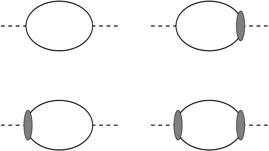
Figure 1: The quark loop contribution to the quadratic form $K_{ij}(P)$, eq.(29), of the effective action of the $\pi_{1}$– and $\pi_{2}$–fields. The solid lines denote the NJL quark propagator. The $\pi_{1}$–field couples to the quarks with a local vertex, the $\pi_{2}$–field through the form factor, $f(k_{\perp})$, represented here by a shaded blob.

A graphical representation of the loop integrals in eq.(29) is given in fig.1. The integral is evaluated by expanding in the meson field momentum, $P$. To order $P^{2}$, one obtains

$$K_{11}(P) = Z_{1}(P^{2}-m_{1}^{2}),\hskip 20.00003ptK_{22}(P)\;\;=\;\;Z_{2}(P^{2}-m_{2}^{2})$$

$$K_{12}(P) = K_{21}(P)\;\;=\;\;\sqrt{Z_{1}Z_{2}}\,\Gamma P^{2}$$ (30)

where

$$Z_{1} = 4I_{2},\hskip 20.00003ptZ_{2}\;=\;4I_{2}^{ff},$$ (31)

$$m_{1}^{2} = Z_{1}^{-1}(-8I_{1}+g^{-1})\;=\;\frac{m^{0}}{Z_{1}gm},$$ (32)

$$m_{2}^{2} = Z_{2}^{-1}(-8I_{1}^{ff}+g^{-1}),$$ (33)

$$\Gamma = \frac{4}{\sqrt{Z_{1}Z_{2}}}I_{2}^{f}.$$ (34)

Here, $I_{n},I_{n}^{f}$ and $I_{n}^{ff}$ denote the usual loop integrals arising in the momentum expansion of the NJL quark determinant, but now with zero, one or two factors $f(k_{\perp})$, eq.(20), in the numerator. We may evaluate them in the rest frame, $k_{\perp}=(0,{\bf k})$,

$$I_{n}^{f..f} \equiv -iN_{\rm c}\int_{\Lambda_{3}}\!\frac{d^{4}k}{(2\pi)^{4}}\frac{f({\bf k})..f({\bf k})}{(m^{2}-k^{2})^{n}}.$$ (35)

The evaluation of these integrals with a 3–momentum cutoff is described e.g. in ref.[16]. The integral over $k_{0}$ is performed by contour integration, and the remaining 3–dimensional integral regularized by the cutoff. Only the divergent parts are kept; all finite parts are dropped. We point out that the momentum expansion of the quark loop integrals, eq.(29), is an essential part of this approach. The NJL–model is understood here as a model only for the lowest coefficients of the momentum expansion of the quark loop, not its full momentum dependence (singularities etc.).

Note that a mixing between the $\pi_{1}$– and $\pi_{2}$–fields occurs only in the kinetic (${\cal O}(P^{2})$–) terms of eq.(30), but not in the mass terms. This is a direct consequence of the definition of the vacuum by eqs.(27, 28), which ensures that the quark loop with one form factor has no $P^{2}$–independent part. The “softness” of the $\pi_{1}$–$\pi_{2}$ mixing causes the $\pi_{1}$–field to decouple at $P^{2}\rightarrow 0$. This property is crucial for the appearance of a Goldstone boson in the chiral limit.

To determine the physical $\pi$– and $\pi^{\prime}$–meson states we have to diagonalize the quadratic part of the action, eq.(24). If one knew the full momentum dependence of the quadratic form, eq.(30), the masses of the physical states would be given as the zeros of the determinant of the quadratic form,

$$\det K_{ij}(P^{2}) = 0,\hskip 56.9055ptP^{2}\;\;=\;\;m_{\pi}^{2},\;m_{\pi^{\prime}}^{2}.$$ (36)

This would be equivalent to the usual Bethe–Salpeter (on–shell) description of bound states: the matrix $K_{ij}(P^{2})$ is diagonalized independently on the respective mass shells, $P^{2}=m_{\pi}^{2},m_{\pi^{\prime}}^{2}$ [9, 17, 19]. In our approach, however, we know the quadratic form, eq.(30), only as an expansion in $P^{2}$ at $P^{2}=0$. It is clear that a determination of the masses according to eq.(36) would be incompatible with the momentum expansion, as the determinant involves ${\cal O}(P^{4})$–terms which are neglected in eq.(30). To be consistent with the $P^{2}$–expansion we must diagonalize the kinetic term and the mass term in eq.(24) simultaneously, with a $P^{2}$–independent transformation of the fields. Let us write eq.(30) in matrix form

$$K_{ij}(P^{2}) = \left(\begin{array}[]{ll}Z_{1}&\sqrt{Z_{1}Z_{2}}\,\Gamma\\ \sqrt{Z_{1}Z_{2}}\,\Gamma&Z_{2}\end{array}\right)P^{2}\;\;-\;\;\left(\begin{array}[]{ll}Z_{1}m_{1}^{2}&\\ &Z_{2}m_{2}^{2}\end{array}\right).$$ (41)

The transformation which diagonalizes both matrices here separately is given by

$$\begin{array}[]{lcrcr}\sqrt{Z_{1}}\pi_{1}^{a}&=&{\displaystyle\frac{\cos\phi}{\sqrt{{Z_{\pi}}}}\pi^{a}}&+&{\displaystyle\frac{m_{2}}{m_{1}}\frac{\sin\phi}{\sqrt{Z_{\pi^{\prime}}}}\pi^{\prime\,a}},\\[2.84544pt] \sqrt{Z_{2}}\pi_{2}^{a}&=&{\displaystyle\frac{m_{1}}{m_{2}}\frac{\sin\phi}{\sqrt{Z_{\pi}}}\pi^{a}}&-&{\displaystyle\frac{\cos\phi}{\sqrt{Z_{\pi^{\prime}}}}\pi^{\prime\,a}},\end{array}$$ (44)

where

$$\tan 2\phi = 2\Gamma\frac{m_{1}}{m_{2}}\left(1-\frac{m_{1}^{2}}{m_{2}^{2}}\right)^{-1},$$ (45)

$$Z_{\pi} = \cos^{2}\phi+\frac{m_{1}^{2}}{m_{2}^{2}}\sin^{2}\phi+2\Gamma\frac{m_{1}}{m_{2}}\cos\phi\sin\phi,$$ (46)

$$Z_{\pi^{\prime}} = \cos^{2}\phi+\frac{m_{2}^{2}}{m_{1}^{2}}\sin^{2}\phi-2\Gamma\frac{m_{2}}{m_{1}}\cos\phi\sin\phi.$$ (47)

In terms of the new fields, $\pi,\pi^{\prime}$, the quadratic part of the action, eq.(24), reads

$$W^{(2)} = {\textstyle{\frac{1}{2}}}\int\!\frac{d^{4}P}{(2\pi)^{4}}\left[\pi^{a}(-P)(P^{2}-m_{\pi}^{2})\pi^{a}(P)+\pi^{\prime\,a}(-P)(P^{2}-m_{\pi^{\prime}}^{2})\pi^{\prime\,a}(P)\right].$$ (48)

Here,

$$m_{\pi}^{2} = \frac{m_{1}^{2}}{Z_{\pi}},\hskip 20.00003ptm_{\pi^{\prime}}^{2}\;\;=\;\;\frac{m_{2}^{2}}{Z_{\pi^{\prime}}}.$$ (49)

The fields $\pi$ and $\pi^{\prime}$ can thus be associated with physical particles.

Let us now consider the chiral limit, i.e., vanishing current quark mass, $m^{0}\rightarrow 0$. From eqs.(31–34) we see that this is equivalent to taking $m_{1}^{2}\rightarrow 0$. (Here and in the following, when discussing the dependence of quantities on the current quark mass, $m^{0}$, we keep the constituent quark mass fixed and assume the coupling constant, $g$, to be changed in accordance with $m^{0}$, such that the gap equation, eq.(28) remains fulfilled exactly. In this way, the loop integrals and eq.(27) remain unaffected by changes of the current quark mass.) Expanding eqs.(49) in $m_{1}^{2}\propto m^{0}$, one finds

$$m_{\pi}^{2} = m_{1}^{2}\;+\;{\cal O}(m_{1}^{4}),$$ (50)

$$m_{\pi^{\prime}}^{2} = \frac{m_{2}^{2}}{1-\Gamma^{2}}\left[1\;+\;\Gamma^{2}\frac{m_{1}^{2}}{m_{2}^{2}}\;+\;{\cal O}(m_{1}^{4})\right].$$ (51)

Thus, in the chiral limit the effective Lagrangian eq.(48) indeed describes a massless Goldstone pion, $\pi$, and a massive particle, $\pi^{\prime}$. Furthermore, in the chiral limit the transformation of the fields, eq.(44), becomes

$$\begin{array}[]{lcrcr}\sqrt{Z_{1}}\pi_{1}^{a}&=&{\displaystyle\left(1-\Gamma^{2}\frac{m_{1}^{2}}{m_{2}^{2}}\right)\pi^{a}}&+&{\displaystyle\frac{\Gamma}{\sqrt{1-\Gamma^{2}}}\left(1+(1-\Gamma^{2})\frac{m_{1}^{2}}{m_{2}^{2}}\right)\pi^{\prime\,a}},\\ \sqrt{Z_{2}}\pi_{2}^{a}&=&{\displaystyle\Gamma\frac{m_{1}^{2}}{m_{2}^{2}}\pi^{a}}&-&{\displaystyle\frac{1}{\sqrt{1-\Gamma^{2}}}\pi^{\prime\,a}}.\end{array}$$ (54)

At $m_{1}^{2}=0$ one observes that $\pi$ has only a component along $\pi_{1}$. This is a consequence of the fact that the $\pi_{1}$–$\pi_{2}$ coupling in the original Lagrangian, eq.(30), is of order $P^{2}$. We remark that, although we have chosen to work with a particular choice of excited–state form factor, eq.(27), the occurence of a Goldstone boson in the chiral limit in eq.(22) is general and does not depend on this choice. This may easily be established using the general gap equations, eqs.(25, 26), together with eq.(29).

4 The axial current

In order to describe the leptonic decays of the $\pi$ and $\pi^{\prime}$ mesons we need the axial current operator. Since our effective action contains besides the pion a field describing an “excited state” with the same quantum numbers, it is clear that the axial current of our model is, in general, not carried exclusively by the $\pi$ field, and is thus not given by the standard PCAC formula. Thus, we must determine the conserved axial current of our model, including the contribution of the $\pi^{\prime}$, from first principles.

In general, the construction of the conserved current in a theory with non-local (momentum–dependent) interactions is a difficult task. This problem has been studied extensively in the framework of the Bethe–Salpeter equation [18] and various 3–dimensional reductions of it such as the quasipotential and the on–shell reduction [20]. In these approaches the derivation of the current is achieved by “gauging” all possible momentum dependence of the interaction through minimal substitution, a rather cumbersome procedure in practice. In contrast, in a Lagrangian field theory a simple method exists to derive conserved currents, the so–called Gell–Mann and Levy method [21], which is based on Noether’s theorem. In this approach the current is obtained as the variation of the lagrgangian with respect to the derivative of a space–time dependent symmetry transformation of the fields. We now show that a suitable generalization of this technique can be employed to derive the conserved axial current of our model with quark–meson form factors depending on transverse momentum.

To derive the axial current we start at quark level. The isovector axial current is the Noether current corresponding to infinitesimal chiral rotations of the quark fields,

$$\psi(x) \rightarrow \left(1-i\varepsilon^{a}{\textstyle{\frac{1}{2}}}\tau^{a}\gamma_{5}\right)\psi(x).$$ (55)

Following the usual procedure, we consider the parameter of this transformation to be space–time dependent, $\varepsilon^{a}\equiv\varepsilon^{a}(x)$. However, this dependence need not be completely arbitrary. To describe the decays of $\pi$ and $\pi^{\prime}$ mesons, it is sufficient to know the component of the axial current parallel to the meson 4–momentum, $P$. It is easy to see that this component is obtained from chiral rotations whose parameter depends only on the longitudinal part of the coordinate

$$\varepsilon^{a}(x) \rightarrow \varepsilon^{a}(x_{||}),\hskip 56.9055ptx_{||}\;\;\equiv\;\;\frac{x\cdot P}{\sqrt{P^{2}}},$$ (56)

since $\partial_{\mu}\varepsilon^{a}(x_{||})\propto P_{\mu}$. In other words, transformations of the form eq.(56) describe a transfer of longitudinal momentum to the meson, but not of transverse momentum. This has the important consequence that the chiral transformation does not change the direction of transversality of the meson–quark interaction, cf. eq.(9). When passing to the bosonized representation, eq.(7), the transformation of the $\pi_{1},\sigma_{1}$– and $\pi_{2},\sigma_{2}$–fields induced by eqs.(55, 56) is therefore of the form

$$\begin{array}[]{lclcl}\pi^{a}_{i}(x)&\rightarrow&\pi^{a}_{i}(x)&+&\varepsilon^{a}(x_{||})\,\sigma_{i}(x),\\ \sigma_{i}(x)&\rightarrow&\sigma_{i}(x)&-&\varepsilon^{a}(x_{||})\,\pi^{a}_{i}(x).\end{array}\hskip 42.67912pt(i=1,2)$$ (59)

This follows from the fact that, for fixed direction of $P$, the vertex eq.(9) describes an instantaneous interaction in $x_{||}$. Thus, the special chiral rotation eq.(56) does not mix the components of the meson fields coupling to the quarks with different form factors.

With the transformation of the chiral fields given by eqs.(59), the construction of the axial current proceeds exactly as in the usual linear sigma model. We write the variation of the effective action, eq.(22), in momentum representation,

$$\delta W = \int\!\frac{d^{4}Q}{(2\pi)^{4}}\varepsilon^{a}(Q)D^{a}(Q),$$ (60)

where $\varepsilon^{a}(Q)=\tilde{\varepsilon}^{a}(Q_{||})\delta^{(3)}(Q_{\perp})$ is the Fourier transform of the transformation eq.(56) and $D^{a}(Q)$ is a function of the fields $\sigma_{i},\pi_{i},i=1,\ldots 2$, given in the form of a quark loop integral,

$$D^{a}(Q) = -iN_{c}\;{\rm tr}\int\!\frac{d^{4}k}{(2\pi)^{4}}\left[\frac{1}{k/\hskip 1.49994pt-m}\delta^{ab}+\frac{1}{k/\hskip 1.49994pt-{\textstyle{\frac{1}{2}}}Q/\hskip 1.49994pt-m}i\gamma_{5}\tau^{a}\frac{1}{k/\hskip 1.49994pt+{\textstyle{\frac{1}{2}}}Q/\hskip 1.49994pt-m}i\gamma_{5}\tau^{b}\sigma_{1}\right]$$ (61)

$$\times(\pi_{1}^{b}(Q)+f(k_{\perp})\pi_{2}^{b}(Q)).$$

Here we have already used that $\sigma_{2}=0$ in the vacuum, eq.(27). Expanding now in the momentum $Q$, making use of eq.(27) and the gap equation, eq.(28), and setting $\sigma_{1}=-m$ (it is sufficient to consider the symmetric limit, $m^{0}=0$), this becomes

$$D^{a}(Q) = -Q^{2}m\left[4I_{2}\pi_{1}^{a}(Q)+4I_{2}^{f}\pi_{2}^{a}(Q)\right]$$ (62)

$$= -Q^{2}m\left[Z_{1}\pi_{1}^{a}(Q)+\sqrt{Z_{1}Z_{2}}\Gamma\pi_{2}^{a}(Q)\right].$$

The fact that $D^{a}(Q^{2})$ is proportional to $Q^{2}$ is a consequence of the chiral symmetry of the effective action, eq.(22). Due to this property, $D^{a}(Q^{2})$ may be regarded as the divergence of a conserved current,

$$A_{\mu}^{a}(Q) = Q_{\mu}m\left[Z_{1}\pi_{1}^{a}(Q)+\sqrt{Z_{1}Z_{2}}\Gamma\pi_{2}^{a}(Q)\right].$$ (63)

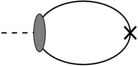
Figure 2: The axial current of the $\pi_{1}$– and $\pi_{2}$–fields, eq.(63), as it follows from Noether’s theorem. The cross denotes the local axial current of the quark field, to which the $\pi_{1}$– and $\pi_{2}$–fields couple through quark loops. Notation is the same as in fig.1.

Eq.(63) is the conserved axial current of our model. It is of the usual “PCAC” form, but contains also a contribution of the $\pi_{2}$ field. The above derivation was rather formal. However, the result can be understood in simple terms, as is shown in fig.2: Both the $\pi_{1}$ and $\pi_{2}$–field couple to the local axial current of the quark field through quark loops; the $\pi_{2}$–field enters the loop with a form factor, $f(k_{\perp})$. The necessity to pull out a factor of the meson field momentum (derivative) means that only the ${\cal O}(P^{2})$–parts of the loop integrals, $I_{2}$ and $I_{2}^{f}$, survive, cf. eq.(35). Chiral symmetry ensures that the corresponding diagrams for the divergence of the current have no $P^{2}$–independent part.

The results of this section are an example for the technical simplifications of working with separable quark interactions. The fact that they can be bosonized by local meson fields makes it possible to apply methods of local field theory, such as Noether’s theorem, to the effective meson action. Furthermore, we note that the covariant (transverse) definition of the 3–dimensional quark interaction, eq.(9), is crucial for obtaining a consistent axial current. In particular, with this formulation there is no ambiguity with different definitions of the pion decay constant as with non–covariant 3-dimensional interactions [9].

5 The weak decay constants of the $\pi$ and $\pi^{\prime}$ meson

We now use the axial current derived in the previous section to evaluate the weak decay constants of the physical $\pi$ and $\pi^{\prime}$ mesons. They are defined by the matrix element of the divergence of the axial current between meson states and the vacuum,

$$\langle 0|\partial^{\mu}A_{\mu}^{a}|\pi^{b}\rangle = m_{\pi}^{2}f_{\pi}\delta^{ab},$$ (64)

$$\langle 0|\partial^{\mu}A_{\mu}^{a}|\pi^{\prime\,b}\rangle = m_{\pi^{\prime}}^{2}f_{\pi^{\prime}}\delta^{ab}.$$ (65)

In terms of the physical fields, $\pi$ and $\pi^{\prime}$, the axial current takes the form

$$A_{\mu}^{a} = P_{\mu}m\sqrt{Z_{1}}\left(\pi^{a}\;+\;\Gamma\sqrt{1-\Gamma^{2}}\,\frac{m_{1}^{2}}{m_{2}^{2}}\,\pi^{\prime\,a}\right)\;+\;{\cal O}(m_{1}^{4}).$$ (66)

Here, we have substituted the transformation of the fields, eq.(54), in eq.(63). The decay constants of the physical $\pi$ and $\pi^{\prime}$ states are thus given by

$$f_{\pi} = \sqrt{Z_{1}}m\;+\;{\cal O}(m_{1}^{4})$$ (67)

$$f_{\pi^{\prime}} = \sqrt{Z_{1}}m\,\Gamma\sqrt{1-\Gamma^{2}}\,\frac{m_{1}^{2}}{m_{2}^{2}}\;+\;{\cal O}(m_{1}^{4}).$$ (68)

The corrections to $f_{\pi}$ due to the inclusion of excited states are of order $m_{\pi}^{4}$. Thus, within our accuracy $f_{\pi}$ is identical to the value obtained with the usual NJL model, $\sqrt{Z_{1}}m$, which follows from the Goldberger–Treiman relation at quark level [6]. On the other hand, the $\pi^{\prime}$ decay constant vanishes in the chiral limit $m^{0}\sim m_{1}^{2}\rightarrow 0$, as expected. We stress that for this property to hold it is essential to consider the full axial current, eq.(63), including the contribution of the $\pi_{2}$–component. As can be seen from eqs.(54, 63), use of the standard PCAC formula $A_{\mu}^{a}\propto\partial_{\mu}\pi_{1}^{a}$ would lead to a non-vanishing result for $f_{\pi^{\prime}}$ in the chiral limit.

The ratio of the $\pi^{\prime}$ to the $\pi$ decay constants can directly be expressed in terms of the physical $\pi$ and $\pi^{\prime}$ masses. From eqs.(67, 68) one obtains, using eqs.(50, 51),

$$\frac{f_{\pi^{\prime}}}{f_{\pi}} = \Gamma\sqrt{1-\Gamma^{2}}\,\frac{m_{1}^{2}}{m_{2}^{2}}\;\;=\;\;\frac{\Gamma}{\sqrt{1-\Gamma^{2}}}\,\frac{m_{\pi}^{2}}{m_{\pi^{\prime}}^{2}}$$ (69)

This is precisely the dependence which was derived from current algebra considerations in a general “extended PCAC” framework [5]. We note that the same behavior of $f_{\pi^{\prime}}$ in the chiral limit is found in models describing chiral symmetry breaking by non-local interactions [9, 17].

The effective Lagrangian illustrates in a compact way the different consequences of axial current conservation for the pion and its excited state. Both matrix elements of $\partial_{\mu}A^{\mu}$, eq.(64) and eq.(65), must vanish for $m^{0}\rightarrow 0$. The pion matrix element, eq.(64) does so by $m_{\pi}^{2}\rightarrow 0$, with $f_{\pi}$ remaining finite, while for the excited pion matrix element the opposite takes place, $f_{\pi^{\prime}}\rightarrow 0$ with $m_{\pi^{\prime}}$ remaining finite.

6 Numerical estimates and conclusions

We can now estimate numerically the excited pion decay constant, $f_{\pi^{\prime}}$, in this model. We take a value of the constituent quark mass of $m=300\,{\rm MeV}$ and fix the 3–momentum cutoff at $\Lambda_{3}=671\,{\rm MeV}$ by fitting the normal pion decay constant $f_{\pi}=93\,{\rm MeV}$ in the chiral limit, as in the usual NJL model without excited states, cf. [16]. With these parameters one obtains the standard value of the quark condensate, $\langle\bar{q}q\rangle=-(253\,{\rm MeV})^{3}$, and $g=0.82\,m^{-2}=9.1\,{\rm GeV}^{-2},\;m^{0}=5.1\,{\rm MeV}$. With the constituent quark mass and cutoff fixed, we can determine the parameter $d$ of the “excited–state” form factor, eq.(20), from the condition eq.(27). We find $d=-1.83\,\Lambda_{3}^{-2}=-4.06\,{\rm GeV}^{-2}$, corresponding to a form factor $f(k_{\perp})$ with a radial node in the range $0\leq|k_{\perp}|\leq\Lambda_{3}$. With this value we determine the $\pi_{1}$–$\pi_{2}$ mixing coefficient, $\Gamma$, eq.(34), as

$$\Gamma = 0.41.$$ (70)

Note that $\Gamma$ is independent of the normalization of the form factor $f(k_{\perp})$, eq.(20). In fact, the parameter $c$ enters only the mass of the $\pi^{\prime}$ meson, cf. eqs.(33, 51); we do not need to determine its value since the result can directly be expressed in terms of $m_{\pi^{\prime}}$. Thus, eq.(69) gives

$$\frac{f_{\pi^{\prime}}}{f_{\pi}} = 0.45\frac{m_{\pi}^{2}}{m_{\pi^{\prime}}^{2}}$$ (71)

For the standard value of the $\pi^{\prime}$ mass, $m_{\pi^{\prime}}=1300\,{\rm MeV}$, this comes to $f_{\pi^{\prime}}=0.48\,{\rm MeV}$, while for a low mass of $m_{\pi^{\prime}}=750\,{\rm MeV}$ one obtains $f_{\pi^{\prime}}=1.46\,{\rm MeV}$. The excited pion leptonic decay constant is thus very small, which is a consequence of chiral symmetry. Note that, as opposed to the qualitative results discussed above, the numerical values here depend on the choice of form factor, eq.(27), and should thus be regarded as a rough estimate.

We remark that the numerical values of the ratio $f_{\pi^{\prime}}/f_{\pi}$ obtained here are comparable to those found in chirally symmetric potential models [17]. However, models describing chiral symmetry breaking by a vector–type confining potential (linear or oscillator) usually understimate the normal pion decay constant by an order of magnitude [9]. Such models should include a short–range interaction (NJL–type), which is mostly responsible for chiral symmetry breaking.

The small value of $f_{\pi^{\prime}}$ does not imply a small width of the $\pi^{\prime}$ resonance, since it can decay hadronically, e.g. into $3\pi$ or $\rho\pi$. Such hadronic decays can also be investigated in the chiral Lagrangian framework set up here. This problem, which requires the evaluation of quark loops with external meson fields of different 4–momenta, will be left for a future investigation.

In conclusion, we have outlined a simple framework for including radial excitations in an effective Lagrangian description of mesons. The Lagrangian obtained by bosonization of an NJL–model with separable interactions exhibits all qualitative properties expected on general grounds: a Goldstone pion with a finite decay constant, and a massive “excited state” with vanishing decay constant in the chiral limit. Our model shows in a simple way how chiral symmetry protects the pion from modifications by excited states, which in turn influences the excited states’ contribution to the axial current. These features are general and do not depend on a particular choice of quark–meson form factor. Furthermore, they are preserved if the derivative expansion of the quark loop is carried to higher orders.

In the investigations described here we have remained strictly within an effective Lagrangian approach, where the coupling constants and field transformations are defined at zero momentum. We have no way to check the quantitative reliability of this approximation for radially excited states in the region of $\sim 1\,{\rm GeV}$, i.e., to estimate the momentum dependence of the coupling constants, within the present model. (For a general discussion of the range of applicability of effective Lagrangians, see [22].) This question can be addressed in generalizations of the NJL model with quark confinement, which in principle allow both a zero–momentum as well as an on–shell description of bound states. Recently, first steps were taken to investigate the full momentum dependence of correlation functions in such an approach [23].

This work was supported partly by the Russian Foundation of Fundamental Research (Grant N 96.01.01223), by the DFG and by COSY (Jülich).

$\pi_{1}\times\partial_{\mu}$   $\hskip 14.22636pt+\hskip 14.22636pt\pi_{2}\times\partial_{\mu}\hskip 2.84544pt$

References

- [1] Review of Particle Properties, Phys. Rev. D 50 (1994) 1198.
- [2] Yu.I. Ivanshin et al., JINR preprint JINR–E1–93–155 (1993).
- [3] C. G. Callan, S. Coleman, J. Wess and B. Zumino, Phys. Rev. 177 (1969) 2247.
-
[4]
For a review, see M. Bando, T. Kugo and K. Yamawaki,
Phys. Rep. 164 (1988) 217;
U.–G. Meissner, Phys. Rep. 161 (1988) 213. - [5] See e.g. C.A. Dominguez, Phys. Rev. D 16 (1977) 2313, and references therein.
-
[6]
D. Ebert and M.K. Volkov, Z. Phys. C 16 (1983) 205;
M.K. Volkov, Ann. Phys. (N.Y.) 157 (1984) 282. - [7] D. Ebert and H. Reinhardt, Nucl. Phys. B 271 (1986) 188.
- [8] C.D. Roberts, R.T. Cahill and J. Praschifka, Ann. Phys. (N.Y.) 188 (1988) 20.
-
[9]
A. Le Yaouanc, L. Oliver, O. Pène and
J.–C. Raynal, Phys. Rev. D 29 (1984) 1233;
A. Le Yaouanc et al., Phys. Rev. D 31 (1985) 137. -
[10]
V.N. Pervushin et al.,
Fortschr. Phys. 38 (1990) 333;
Yu.L. Kalinovsky et al., Few–Body Systems 10 (1991) 87. - [11] M.A. Nowak and I. Zahed, Phys. Rev. D 48 (1993) 356.
- [12] S. Schmidt, D. Blaschke and Yu.L. Kalinovsky, Phys. Rev. C 50 (1994) 435.
- [13] A.A. Andrianov and V.A. Andrianov, Int. J. Mod. Phys. A 8 (1993) 1981; Nucl. Phys. B (Proc. Suppl.) 39 B, C (1993) 257.
- [14] Yu.L. Kalinovsky, L. Kaschluhn and V.N. Pervushin, Phys. Lett. B 231 (1989) 288.
- [15] R.P. Feynman, M. Kislinger and F. Ravndal, Phys. Rev. D 3 (1971) 2706.
- [16] D. Ebert, Yu.L. Kalinovsky, L. Münchow and M.K. Volkov, Int. J. Mod. Phys. A 8 (1993) 1295.
- [17] Yu.L. Kalinovsky and C. Weiss, Z. Phys. C 63 (1994) 275.
- [18] F. Gross and D.O. Riska, Phys. Rev. C 36 (1987) 1928.
- [19] H. Ito, W.W. Buck and F. Gross, Phys. Rev. C 45 (1992) 1918.
- [20] H. Ito, W.W. Buck and F. Gross, Phys. Rev. C 43 (1991) 2483.
- [21] M. Gell–Mann and M. Levy, Nuovo Cim. 16 (1960) 53.
- [22] R.L. Jaffe and P.F. Mende, Nucl. Phys. B 369 (1992) 189.
- [23] L.S. Celenza et al., Phys. Rev. D 51 (1995) 3638.