Abstract

We discuss an application of QCD sum rules to the heavy baryons $\Lambda_{Q}$ and $\Sigma_{Q}$. The predictions for the masses of heavy baryons, residues and Isgur-Wise function are presented. The new results on two loop anomalous dimensions of baryonic currents and QCD radiative corrections (two- and three- loop contributions) to the first two Wilson coefficients in OPE are explicitly presented.

1 Introduction

Baryons with one $b$ quark are very nice systems for application of Heavy Quark Effective Theory (HQET)[1]. It allows one to organize the determination of the properties of baryons in an $1/m_{Q}$-expansion, the leading term of which gives rise to the spin-flavour symmetry. Well known predictions of the HQET are the relations between different hadron transition form factors. For example, the six form-factors describing the $\Lambda_{b}\to\Lambda_{c}$ electro-weak transitions are reduced to one universal Isgur-Wise function $\xi(v\cdot v^{\prime})$ in the HQ limit [2, 3, 4]. However, one still remains with many non-perturbative parameters, such as the mass of the baryon, the Isgur-Wise function and the averaged kinetic and magnetic energy of the baryon, which should be estimated by using some non-perturbative method as sum rules [5], lattice calculation or some potential model.

In the present paper we review an application of the QCD sum rule method to calculate the masses, residues of heavy baryons and baryonic Isgur-Wise function[11, 12, 13, 14, 15, 16, 17, 18, 19, 20, 22, 23, 24].

2 Currents, anomalous dimensions and residues

The currents of the heavy baryon $\Lambda_{Q}$ and the heavy quark spin baryon doublet $\{\Sigma_{Q},\Sigma_{Q}^{*}\}$ are associated with the spin-parity quantum numbers $j^{P}=0^{+}$ and $j^{P}=1^{+}$ for the light diquark system with antisymmetric and symmetric flavor structure, respectively. Adding the heavy quark to the light quark system, one obtains $j^{P}=\frac{1}{2}^{+}$ for the $\Lambda_{Q}$ baryon and the pair of degenerate states $j^{P}=\frac{1}{2}^{+}$ and $j^{P}=\frac{3}{2}^{+}$ for the baryons $\Sigma_{Q}$ and $\Sigma_{Q}^{*}$. The general structure of the heavy baryon currents has the form (see e.g. [14] and refs. therein)

$$J=[q^{iT}C\Gamma\tau q^{j}]\Gamma^{\prime}Q^{k}\epsilon_{ijk}.$$ (1)

Here the index $T$ means transposition, $C$ is the charge conjugation matrix with the properties $C\gamma^{T}_{\mu}C^{-1}=-\gamma_{\mu}$ and $C\gamma^{T}_{5}C^{-1}=\gamma_{5}$, $i,j,k$ are colour indices and $\tau$ is a matrix in flavour space. The effective static field of the heavy quark is denoted by $Q$. For each of the ground state baryon currents there are two independent current components $J_{1}$ and $J_{2}$:

$$J_{\Lambda 1} = [q^{iT}C\tau\gamma_{5}q^{j}]Q^{k}\varepsilon_{ijk},\qquad J_{\Lambda 2}\ =\ [q^{iT}C\tau\gamma_{5}\gamma_{0}q^{j}]Q^{k}\varepsilon_{ijk},$$

$$J_{\Sigma 1} = [q^{iT}C\tau\vec{\gamma}q^{j}]\cdot\vec{\gamma}\gamma_{5}Q^{k}\varepsilon_{ijk},\qquad J_{\Sigma 2}\ =\ [q^{iT}C\tau\gamma_{0}\vec{\gamma}q^{j}]\cdot\vec{\gamma}\gamma_{5}Q^{k}\epsilon_{ijk}.$$ (2)

The anomalous dimensions of the heavy baryon currents up to second order was calculated recently in [22] and read (for example in the MS scheme with naively anticommuting $\gamma_{5}$)

$$\gamma_{\Lambda 1}=-8\left(\frac{\alpha_{s}}{4\pi}\right)+\frac{1}{9}(16\zeta(2)+40N_{F}-796)\left(\frac{\alpha_{s}}{4\pi}\right)^{2},$$ (3)

$$\gamma_{\Lambda 2}=-4\left(\frac{\alpha_{s}}{4\pi}\right)+\frac{1}{9}(16\zeta(2)+20N_{F}-322)\left(\frac{\alpha_{s}}{4\pi}\right)^{2},$$ (4)

$$\gamma_{\Sigma 1}=-4\left(\frac{\alpha_{s}}{4\pi}\right)+\frac{1}{9}(16\zeta(2)+20N_{F}-290)\left(\frac{\alpha_{s}}{4\pi}\right)^{2},$$ (5)

$$\gamma_{\Sigma 2}=-\frac{8}{3}\left(\frac{\alpha_{s}}{4\pi}\right)+\frac{1}{27}(48\zeta(2)+8N_{F}+324)\left(\frac{\alpha_{s}}{4\pi}\right)^{2}.$$ (6)

The anomalous dimensions are ingredient of renormalization group invariant sum rules. Numerically effects of $\gamma_{2}$ are very small and gives about $1-2\%$ corrections to the current redefinition.

Let us define residues $F_{i}(\mu)$ ($i=\Lambda,\Sigma$) of the baryonic currents according to

$$\langle 0|J(\mu)|\Lambda_{Q}\rangle=F_{\Lambda}(\mu)u,\qquad\langle 0|J(\mu)|\Sigma_{Q}\rangle=F_{\Sigma}(\mu)u,$$ (7)

where $u$ is spinor. Then we define bound state energy $E_{R}$ of the baryon $R$ and use the formula

$$m_{\rm baryon}=m_{Q}+E_{R}+\frac{c}{m_{Q}}+O(1/m^{2}_{Q}),$$ (8)

where $m_{Q}$ is the running heavy quark mass at the scale of the same mass and $c$ is a coefficient connected with the averaged kinetic and magnetic energy in the baryonic state. The coefficient $c$ was recently estimated in [17] by using QCD sum rules.

3 Correlator of two baryonic currents

In order to obtain information about the value of the mass of the baryon and its residue one considers the correlator of two baryonic currents

$$\Pi(\omega=k\cdot v)=i\int d^{4}xe^{ikx}\langle 0|TJ(x)\bar{J}(0)|0\rangle,$$ (9)

where $k_{\mu}$ and $v_{\mu}$ are the residual momentum and four velocity in $p_{\mu}=m_{Q}v_{\mu}+k_{\mu}$, respectively. $P(\omega)$ can be factorized into a spinor dependent piece and scalar function $P(\omega)$ according to

$$\Pi(\omega)=\Gamma^{\prime}\frac{1+v\kern-5.0pt\raise 1.0pt\hbox{$\scriptstyle/$}\kern 1.0pt}{2}\bar{\Gamma}^{\prime}\frac{1}{4}\mathop{\rm Tr}\nolimits(\Gamma\bar{\Gamma})2\mathop{\rm Tr}\nolimits(\tau\bar{\tau})P(\omega).$$ (10)

The correlator function $P_{\rm OPE}(\omega)$ satisfies the dispersion relation

$$P_{\rm OPE}(\omega)=\int_{0}^{\infty}\frac{\rho(\omega^{\prime})d\omega^{\prime}}{\omega^{\prime}-\omega-i0}+\hbox{\rm subtraction},$$ (11)

where $\rho(\omega)={\sl Im}(P(\omega))/\pi$ is the spectral density.

Following the standard QCD sum rules method [5] the correlator is calculated in the region $-\omega\approx 1-2{\,\sl GeV}$, including perturbative and non-perturbative effects, where non-perturbative effects can be quite important. The non-perturbative effects are taken into account with the help of an operator product expansion. The OPE of two point correlator was discussed in Refs. [11, 12, 13, 14, 16]. $1/m_{Q}$ corrections to two and three point correlators were calculated in [19, 20, 17]. The leading perterbative term and the next-to-leading term in OPE (gluon condensate contribution) give the spectral densities

$$\rho_{0}(\omega)=\frac{\omega^{5}}{20\pi^{4}},\quad\rho_{4}(\omega)=c\frac{\alpha_{s}\langle GG\rangle}{32\pi^{3}}\omega.$$ (12)

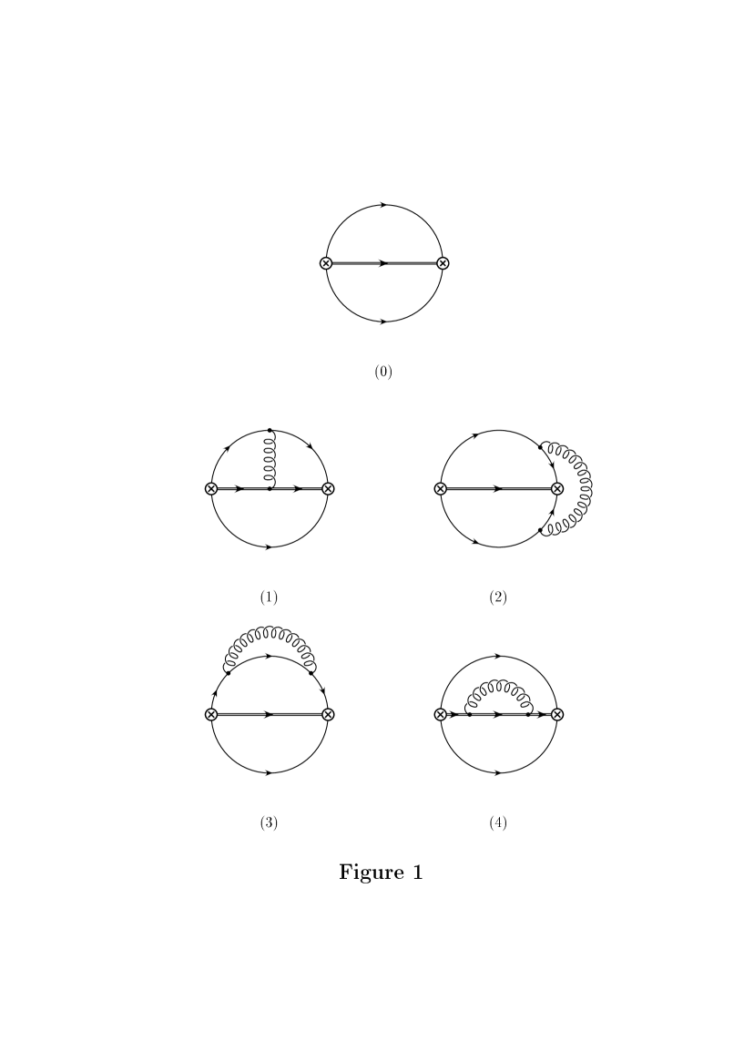
Figure 1: Two-loop and three-loop contributions to the correlator of two heavy baryon currents. (0) two loop lowest order contribution, (1)-(4) three loop $O(\alpha_{S})$ contributions.

Next we consider the radiative corrections to the spectral density of the perturbative contribution. There are four different graphs contributing to the correlator, which are shown in Fig. 1. The fact that all graphs in Fig. 1 have two-point two-loop subgraphs greatly simplifies the calculational task. One can first evaluate the respective subgraphs which leaves one with a one-loop integration. The first two-loop integration can be performed by using algebraic method described in [21]. It is important to note that the results of the two-loop integration are polynomials of the external momentum relative to this subgraph. Hence, the last integration is really a one-loop one, but the power of one of the propagators becomes a non-integer number. The evaluation of results in a Taylor expansion in $1/\epsilon$ gives [24]

$$P(\omega)\!\! = \!\!-\frac{32\omega^{5}}{(4\pi)^{4}}\Bigg{[}\left(\frac{-2\omega}{\mu}\right)^{-4\epsilon}\frac{1}{40}\Bigg{(}\frac{1}{\epsilon}+\frac{107}{15}\Bigg{)}$$

$$+\frac{\alpha_{S}}{4\pi}\left(\frac{-2\omega}{\mu}\right)^{-6\epsilon}\Bigg{(}\frac{n^{2}-4n+6}{45\epsilon^{2}}+\frac{40\zeta(2)+61n^{2}-234n+396}{225\epsilon}+\frac{(n-2)s}{90}$$

$$+\frac{5(195n^{2}-780n+1946)\zeta(2)-2200\zeta(3)+4907n^{2}-18408n+34352}{2250}\Bigg{)}\Bigg{]}.$$

Here we assume that matrix $\Gamma_{1}$ in Eq.(1) is an antisymmetrized product of $n$ Dirac matrices: $\Gamma=\gamma^{[\mu_{1}}\cdots\gamma^{\mu_{n}]}$. This introduces a $n$- and $s$-dependence in the QCD corrections due to the identities

$$\gamma_{\alpha}\Gamma\gamma_{\alpha}=h\Gamma=(-1)^{n}(D-2n)\Gamma,\qquad\gamma_{0}\Gamma\gamma_{0}=(-1)^{n}s\Gamma.$$ (14)

The correlator is renormalized by the renormalization factor of the baryonic current, which is derived in [14],

$$P(\omega)=Z^{2}_{J}P^{\rm ren}(\omega)\qquad\hbox{\rm with\ }Z_{J}=1+\frac{\alpha_{S}C_{B}}{4\pi\epsilon}(n^{2}-4n+6).$$ (15)

The multiplication with $Z^{2}_{J}$ results in the cancelation of the second power in $1/\epsilon$. The first power in $1/\epsilon$ is purely real and hence does not contribute to the spectral density. The renormalized spectral density $\rho^{\rm ren}(\omega)={\sl Im}(P^{\rm ren}(\omega))/\pi$ must in fact be finite and can be read immediately off Eq. (3),

$$\rho^{\rm ren}(\omega) = \rho_{0}(\omega)\Bigg{[}1+\frac{\alpha_{S}}{\pi}r(\omega/\mu)\Bigg{]},\quad\mbox{where}\quad\rho_{0}(\omega)\ =\ \frac{\omega^{5}}{20\pi^{4}}\quad\mbox{and}$$ (16)

$$r(\omega/\mu) = \frac{2}{3}(n^{2}-4n+6)\ln\left(\frac{\mu}{2\omega}\right)+\frac{2}{45}(60\zeta(2)+38n^{2}-137n+273).$$

The $\alpha_{S}$ correction can be seen to depend on the properties of the light-side Dirac matrix in the heavy baryon current. The results in the naively anticommuting $\gamma_{5}$-scheme (AC) are

$$r_{\Lambda 1}(\omega/\mu)\!\! = \!\!4\ln\left(\frac{\mu}{2\omega}\right)+\underbrace{\frac{2(20\zeta(2)+91)}{15}}_{\approx 16.51},$$ (17)

$$r_{\Lambda 2,\Sigma 1}(\omega/\mu) = 2\ln\left(\frac{\mu}{2\omega}\right)+\underbrace{\frac{4(10\zeta(2)+29)}{15}}_{\approx 12.12},$$

$$r_{\Sigma 2}(\omega/\mu)\!\! = \!\!\frac{2}{3}ln\left(\frac{\mu}{2\omega}\right)+\underbrace{\frac{2(60\zeta(2)+151)}{45}}_{\approx 11.10}.$$

The coefficient of the logarithmic term $\ln(2\omega/\mu)$ in Eq. (16) coincides with twice the one-loop anomalous dimension given in Eq. (15), as expected. The results for the Baryons $\Lambda_{1}$ and $\Lambda_{2}$ in the ’t Hooft-Veltman $\gamma_{5}$-scheme (HV) differ from those presented above. But we know that currents in different schemes should be connected by finite renormalization factors $Z$, $J_{AC}=ZJ_{HV}.$ Such factors was recently derived from two-loop anomalous dimensions of baryonic currents [22]. They read

$$Z_{\Lambda 1}=1-\frac{4\alpha_{S}}{3\pi}\quad\mbox{and}\quad Z_{\Lambda 2}=1-\frac{2\alpha_{S}}{3\pi}.$$ (18)

By multiplying the results in the ’t Hooft-Veltman scheme by $Z^{2}$ we obtain the same results as in the naively anticommuting $\gamma_{5}$-scheme.

The results show that the $\alpha_{S}$-corrections amount to about 100%, which makes perturbative QCD radiative “corrections” very important in QCD sum rules. We used $\mu=2\omega\approx 1{\,\sl GeV}$ and $\alpha_{S}(\mu)=0.3$.

4 Contribution of quark condensate

Next, we consider the contribution of the quark condensate, which appears in the nondiagonal sum rules. The leading and next-to-leading spectral density are

$$\rho(\omega)=-\frac{\langle\bar{q}q\rangle}{\pi^{2}}\omega^{2}\qquad\rho_{5}(\omega)=2\Big{(}1-\frac{c}{2}\Big{)}\frac{\langle\bar{q}q\rangle m^{2}_{0}}{16\pi^{2}}.$$ (19)

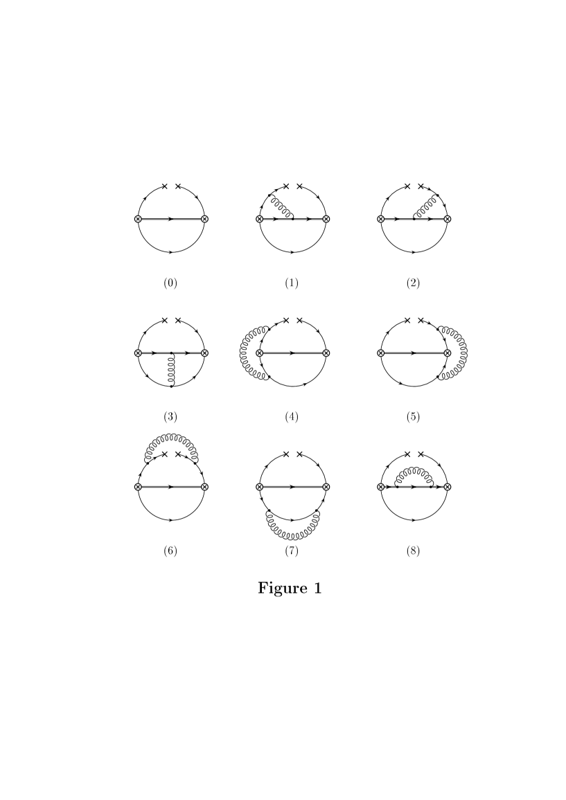
Figure 2: One-loop and two-loop contributions to the nondiagonal correlator of two heavy baryon currents. (0) one loop lowest order contribution, (1)-(8) two loop $O(\alpha_{S})$ contributions.

The radiative corrections to the quark condensate term can be quite important, and we take it into account. There are 8 different graphs contributing to the correlator, which are shown in Fig. 2. We used the same method as we used for the perturbative term. The correlator must be renormalized by the renormalization factor of the baryonic current [14] and quark condensate,

$$P(\omega)=Z_{J_{1}}Z_{J_{2}}Z_{\bar{q}q}P^{\rm ren}(\omega)\qquad\hbox{\rm with\ }Z_{J_{1}}=1+\frac{\alpha_{S}C_{B}}{4\pi\epsilon}(n^{2}-4n+6),$$ (20)

$$Z_{J_{2}}=1+\frac{\alpha_{S}C_{B}}{4\pi\epsilon}((n-2+s)^{2}+2),\qquad Z_{\bar{q}q}=1+\frac{\alpha_{S}}{4\pi\epsilon}(-3).$$ (21)

This procedure cancels the second power in $1/\epsilon$ while the first power in $1/\epsilon$ is purely real and does not contribute to the spectral density. For the renormalized spectral density we get

$$\rho^{\rm ren}(\omega) = -\frac{\langle\bar{q}q\rangle^{\rm ren}\omega^{2}}{\pi^{2}}\Big{[}1+\frac{\alpha_{s}}{4\pi}\Big{(}\frac{4}{3}(2n^{2}-8n+7+2(n-2)s)\ln\left(\frac{\mu}{2\omega}\right)$$ (22)

$$+\frac{2}{3}(8n^{2}-28n+37+8ns-14s+8\zeta(2))\Big{)}\Big{]}.$$

Then we proceed with the usual QCD sum rules analysis and equate the theoretical result for $P_{\rm OPE}(\omega)$ with the dispersion integral over the hadron states saturated by the lowest lying state with the bound state energy $E_{R}$ plus exited states and continuum. So the phenomenological part of the sum rule is given by the spectral density $\rho_{\rm ph}(\omega)=\rho_{\rm res}(\omega)+\rho_{\rm cont}(\omega),$ where the contribution $\rho_{\rm res}$ of the low-lying baryon state is $\rho_{\rm res}(\omega)=\frac{|F|^{2}}{2}\delta(\omega-E_{R}).$ As is usual for the contribution of excited states and continuum contributions we assume hadron-parton duality and take $\rho_{\rm cont}(\omega)=\theta(\omega-E_{C})\rho(\omega)$, where $\rho$ is the result of the OPE calculations. We apply the Borel transformation

$$\hat{B}_{T}=\lim\frac{\omega^{n}}{\Gamma(n)}\left(-\frac{d}{d\omega}\right)^{n}\qquad n,-\omega\to\infty,\quad T=-\omega/n\hbox{\rm\ fixed}$$ (23)

and finally obtain the sum rule

$$\frac{1}{2}F^{2}e^{-E_{R}/T}=\int_{0}^{E_{C}}\rho(\omega^{\prime})e^{-\omega^{\prime}/T}d\omega^{\prime}+\hat{B}P_{\rm pc}(T).$$ (24)

5 Numerical results

Let us discuss the sum rule analysis. First, we analyse the dependence of the bound state energy $E_{R}$ as a function of the energy of continuum $E_{C}$ and the Borel parameter $T$ in a wide region of these arguments and try to find regions of stability in $T$ and $E_{c}$. Second, we fix the energy of continuum $E_{c}=E_{c}^{\rm best}$ by requiring that $E_{R}(T)$ should have the highest possible stability in its dependence on the Borel parameter $T$. We take into account the $\alpha_{S}$-correction to the spectral density and obtain

$$E_{\Lambda}=0.9\pm 0.2{\,\sl GeV}\qquad\hbox{\rm and}\qquad E_{C}^{\rm best}=1.2\pm 0.2{\,\sl GeV}.$$ (25)

The analysis of sum rules at $E_{\Lambda}=0.9{\,\sl GeV}$ gives for the $\Lambda$-residue

$$F_{\Lambda}=(0.03-0.04){\,\sl GeV}^{3}\qquad\hbox{\rm and}\qquad E_{C}=1.0-1.4{\,\sl GeV}.$$ (26)

Doing the same analysis for the $\Sigma$ baryon and taking into account the $\alpha_{S}$-corrections we obtain

$$E_{\Sigma}=1.1\pm 0.2{\,\sl GeV}\qquad\hbox{\rm and}\qquad E_{C}^{\rm best}=1.4\pm 0.2{\,\sl GeV}.$$ (27)

$$F_{\Sigma}=(0.045-0.055){\,\sl GeV}^{3}\qquad\hbox{\rm and}\qquad E_{C}^{\rm best}=1.4\pm 0.2{\,\sl GeV}.$$ (28)

All the results are summarized in the Table 1 , where we compare our results with the leading order results obtained in the [14, 17, 19] and some experimental values.

	Exp. [26] and
	Pot.model [25]	[14]	[17]	[19]	L.O.	N.L.O.
$E_{C}(\Lambda)$		$1.20$	$1.2\pm 0.1$	$1.20\pm 0.15$	$1.2\pm 0.2$	$1.2\pm 0.2$
$E_{C}(\Sigma)$		$1.46$	$1.4\pm 0.1$	$1.30\pm 0.15$	$1.4\pm 0.2$	$1.4\pm 0.2$
$E_{R}(\Lambda)$	$0.840$($1.040$)	$0.78$	$0.9\pm 0.1$	$0.79\pm 0.05$	$0.8\pm 0.2$	$0.92\pm 0.2$
$E_{R}(\Sigma)$	$1.050$($1.250$)	$0.99$		$0.96\pm 0.05$	$1.02\pm 0.2$	$1.12\pm 0.2$
Diff.	$0.190$	$0.21$		0.17	$0.2$	$0.2$
$\Delta(\Lambda)$	$0.460$				$0.40\pm 0.05$	$0.32\pm 0.05$
$\Delta(\Sigma)$	$0.405$				$0.38\pm 0.05$	$0.32\pm 0.05$
$F_{\Lambda}$		$2.3\pm 0.5$	$2.5\pm 0.5$	$1.7\pm 0.6$	$2.4\pm 0.5$	$3.2\pm 0.5$
$F_{\Sigma}$		$3.5\pm 0.6$	$4.0\pm 0.5$	$4.1\pm 0.6$	$3.4\pm 0.5$	$5.2\pm 0.5$

Table 1: All energies like $E_{C}$, $E_{R}$ and $\Delta$ are given in ${\,\sl GeV}$, the residues in $10^{-2}{\,\sl GeV}^{3}$. The value of the Borel parameter is $T=0.6{\,\sl GeV}$. We use $m_{b}=4800{\,\sl MeV}$ (resp. $4600{\,\sl MeV}$) in the first colomn.

6 The Isgur-Wise function

Next, we consider semileptonic transition $\Lambda_{b}\to\Lambda_{c}$. The matrix elements of the weak current for $\Lambda_{b}\to\Lambda_{c}$ at the leading order $1/m_{Q}$ are determined only by Isgur-Wise function

$$<\Lambda_{c}|\bar{c}\Gamma b|\Lambda_{b}>=\xi(y)\bar{u}_{c}\Gamma u_{b}.$$ (29)

where $y=v_{b}\cdot v_{c}$ and $\Gamma$ is some gamma matrix. The Isgur-Wise function was calculated in Ref.[15] by using three-point QCD sum rules. The slope of Isgur-Wise function at y=1 is

$$\rho^{2}=-1.15\pm 0.2.$$ (30)

The uncertainty is connected mainly with an assumption about continuum model. We have found that the shape of the Isgur-Wise function nearly coincides with the ansatz formula

$$\xi(y)=\frac{2}{y+1}exp[(2\rho^{2}-1)\frac{y-1}{y+1}],$$ (31)

with the slope in Eq.(30). Fig.3 shows the Isgur-Wise function at different energies of the continuum ($E_{c}=1.0,1.2,1.4GeV$). $1/m_{Q}$ corections to $\Lambda_{b}\to\Lambda_{c}$ transition were discussed recently in [20]. The important $1/m_{Q}$ effects to the decay come only from the weak current expansion.

7 Conclusions

We have calculated one and two-loop anomalous dimensions of baryonic currents. We have studied the expansion of the correlator of two heavy baryon currents at small Euclidian distances. The radiative corrections to the first two Wilson coefficients are calculated. The heavy baryons sum rules in $\alpha_{S}$ order are derived. The predictions for the mass, residues , the slope and shape of Isgur-Wise function are presented.

8 Acknowledgments

This work was partially supported by the BMBF, FRG, under contract 06MZ566, and by the Human Capital and Mobility program under contract CHRX-CT94-0579. I would like to thank A.G. Grozin, J.G. Körner and S.Groote for collaboration. I am grateful to organizers of the seminar ”Heavy Quark Physics”.

9 References

Figure 3: The Isgur-Wise function.

References

• [1] See for example: M.Neubert Physics Report V245 N5-6, (1994)
• [2] H. Georgi, Nucl. Phys. B363 (1991) 301
• [3] T. Mannel, W. Roberts, Z. Ryzak, Nucl. Phys. B355 (1991) 38
• [4] F. Hussein, J.G. Körner, M. Krämer and G. Thompson, Z. Phys. C51 (1991) 321
• [5] M.A. Shifman, A.I. Vainstein and V.I. Zakharov,
Nucl. Phys. B147 (1979) 385; B147 (1979) 488
• [6] B.L. Ioffe, Nucl. Phys. B188 (1981) 317; Errata B191 (1981) 591
• [7] V.M. Belyaev and B.L. Ioffe, ZhETF 83 (1982) 876
• [8] Y. Chung, H.G. Dosch, M. Kremer and P. Schall, Nucl. Phys. B197 (1981) 55
• [9] A.A. Pivovarov and L.R. Surguladze, Nucl. Phys. B360 (1991) 97
• [10] A.A. Ovchinnikov, A.A. Pivovarov and L.R. Surguladze,
Int. J. Mod. Phys. A6 (1991) 2025
• [11] E.V. Shuryak, Nucl. Phys. B198 (1982) 83
• [12] B.Y. Block and V.L.Eletsky, Z. Phys. C30 (1986) 151; C30 (1986) 229
• [13] E. Bagan, M. Chabab, H.G. Dosch and S. Narison,
Phys. Lett. B278 (1992) 367; B287 (1992) 176
• [14] A.G. Grozin and O.I. Yakovlev, Phys. Lett. B285 (1992) 254
• [15] A.G. Grozin and O.I. Yakovlev, Phys. Lett. B291 (1992) 441
• [16] E. Bagan, M. Chabab, H.G. Dosch and S. Narison,
Phys. Lett. B301 (1993) 243
• [17] P. Colangelo, C.A. Dominguez, G. Nardulli and N. Paver,
BARI-TH/95-219, hep-ph/9512334
• [18] P. Colangelo and F. De Fazio, BARI-TH/95-230, hep-ph/9604425
• [19] Y.B. Dai, C.S. Huang, C. Liu and C.D. Lü, Phys. Lett. B 371 (1996) 99
• [20] Y.B. Dai, C.S. Huang, M. Huang, C. Liu, hep-ph/9608277
• [21] D. Brodhurst and A.G. Grozin, Phys. Lett. B267 (1991) 105
• [22] S. Groote, J.G. Körner and O.I. Yakovlev,
hep-ph/9604386, to be published in Phys. Rev. D
• [23] S. Groote, J.G. Körner and O.I. Yakovlev, Mainz Preprint MZ/TH-96-21
• [24] S. Groote, J.G. Körner and O.I. Yakovlev, (in preparation) , will be published
• [25] S. Capstick and N. Isgur, Phys. Rev. D34 (1986) 2809
• [26] UA1 Collab., C. Aldajar et al., CERN PPE/91-202 (1991)
Refer to caption