MC-Simulation of the
Transverse Double Spin Asymmetry for RHIC

Abstract

Using Sphinx tt, a new MC simulation program for transverse polarized nucleon–nucleon scattering based on Pythia 5.6, we calculate the transverse double spin asymmetry $A^{TT}$ in the Drell-Yan process. If one assumes (quite arbitrarily) that the transversity parton distribution $\delta q(x,Q^{2})$ equals the helicity distribution $\Delta q(x,Q^{2})$ at some low $Q_{0}^{2}$ scale, the resulting asymmetry is of order 1%. In this case is $A^{TT}$ would hardly be be measurable with PHENIX at RHIC.

1 Introduction

Originally, the transversity parton distribution $\delta q(x,Q^{2})$ was defined by Ralston and Soper [1]. However, only after polarized targets were developped and first spin-experiments yielded very interesting results, transverse spin structure functions became a real issue. After the “rediscovery” of $\delta q(x,Q^{2})$ by Artru and Mekhfi [2] in 1990 the topic of transverse spin has gained an increasing amount of attention by elementary particle physicists. Much of the interest is caused by the fact that besides the well known unpolarized and helicity weighted parton distributions $q(x,Q^{2})$ and $\Delta q(x,Q^{2})$ the transversity distribution $\delta q(x,Q^{2})$ is the only twist-2 distribution of the nucleon. On the other hand, its special chirality selection rules prevent its measurement at leading order in polarized inclusive deep inelastic lepton–proton scattering experiments and therefore no experimental data on $\delta q(x,Q^{2})$ is available up to now. This situation is expected to change in the near future, when the Relativistic Heavy Ion Collider (RHIC) at Brookhaven National Laboratory will be able to scatter transversely polarized protons with high cm energy, luminosity, and large polarization of each beam. One of the proposed experiments for the RHIC spin program is the measurement of the transverse double spin asymmetry

$$A^{TT}=\frac{{\rm d}\sigma^{\uparrow\uparrow}-{\rm d}\sigma^{\uparrow\downarrow}}{{\rm d}\sigma^{\uparrow\uparrow}+{\rm d}\sigma^{\uparrow\downarrow}}$$ (1)

using the Drell–Yan process $q_{i}\bar{q}_{i}\rightarrow l^{+}l^{-}$ [3, 4, 5], where $i$ denotes the flavour and $l^{+}l^{-}$ an electron-positron or muon pair. Here, the asymmetry is not suppressed because the two quark lines in the unitarity diagram are independent of each other [2]. This also holds for other partonic processes, like the prompt photon production with an away-side jet $q_{i}+\bar{q}_{i}\rightarrow\gamma g$, or two-jet production $q_{i}+\bar{q}_{i}\rightarrow gg$, $q_{i}q_{i}\rightarrow q_{i}q_{i}$. Nonetheless, these reactions are not very useful for extracting information about the transversity distribution, since either the partonic part of the asymmetry is small or the cross section of other contributing background processes is much larger [6, 7].

It is generally believed, that at some low scale $Q_{0}$ the transversity distribution is similar to the helicity distribution

$$\delta q(x,Q_{0}^{2})\simeq\Delta q(x,Q_{0}^{2})$$ (2)

and that their difference is only due to dynamic effects [8, 9]. Crude analytical estimates which were based on this assumption yielded $A^{TT}\sim 10\%$ [6, 10]. However, in these model calculations the correct $Q^{2}$–evolution of $\delta q(x,Q^{2})$ was not taken into account.

In this paper we present a new estimate of the transverse double spin asymmetry of the Drell-Yan process based on (2) using the new MC simulation program Sphinx tt. We take into account the correct $Q^{2}$–evolution and give a crude estimate for the QCD corrections to the simple Drell-Yan model.

In section 2 we describe the model we used for our calculations. Section 3 contains a short description of Sphinx tt. Our results and conclusions are presented in section 4.

2 Our model

In order to be able to make an estimate of $A^{TT}$ we assume that the transversity weighted distribution of quarks and antiquarks equals the helicity weighted distribution at the low scale $Q_{0}^{2}=4$ GeV²:

$$\delta q(x,4\;{\rm GeV}^{2})=\Delta q(x,4\;{\rm GeV}^{2}),\quad\delta\bar{q}(x,4\;{\rm GeV}^{2})=\Delta\bar{q}(x,4\;{\rm GeV}^{2})\quad.$$ (3)

This is rather an ad hoc assumption. Transversity distributions and helicity distributions should agree for some very small $Q^{2}$, where perturbative QCD is not applicable. It is not clear how much they will differ after evolution up to 4 GeV². Their DGLAP equations differ most notably because the transversity distribution is not a singlett with respect to chirality and therefore does not couple to gluons. Its evolution equation reads simply

$$\frac{{\rm d}}{{\rm d}\ln Q^{2}}\delta q_{i}(x,Q^{2})=\frac{\alpha_{s}(Q^{2})}{2\pi}\int_{x}^{1}\frac{{\rm d}y}{y}\delta q_{i}(y,Q^{2})\;\delta P_{qq}\left(\frac{x}{y}\right)\quad.$$ (4)

The splitting function $\delta P_{qq}(z)=C_{2}(R)[2/(1-z)_{+}-2+(3/2)\delta(z-1)]$ was calculated by Artru and Mekhfi [2]. Equation (4) implies for the anomalous dimensions

$$\delta q^{(n)}_{i}(Q^{2}) = \int_{0}^{1}{\rm d}x\;x^{n-1}\delta q_{i}(x,Q^{2})\quad,$$ (5)

$$\delta P_{qq}^{(n)} = \int_{0}^{1}{\rm dz}\;z^{n-1}\delta P_{qq}(z)=C_{2}(R)\left(\frac{3}{2}-2\sum_{j=1}^{n}\frac{1}{j}\right)\quad,$$ (6)

$$\delta q_{i}^{(n)}(Q^{2}) = \delta q_{i}^{(n)}(Q_{0}^{2})\left(\frac{\alpha_{s}(Q_{0}^{2})}{\alpha_{s}(Q^{2})}\right)^{\delta P^{(n)}_{qq}/2\pi b}\quad.$$ (7)

Since $b=(33-2n_{f})/12\pi>0$, $\delta P_{qq}^{(n)}<0$ and $\delta P_{qq}^{(n+1)}<\delta P_{qq}^{(n)}$ all momenta of the transversity distribution decrease and the distribution becomes softer with increasing $Q^{2}$.

We used the leading-order parametrizations Set C of Gehrmann/Stirling [12], and Bartelski/Tatur [13] and evolved them according to (4).

The authors of all major previous works [1, 2, 6, 8, 11] about the transverse double spin asymmetry of lepton pair production only considered the simple electromagnetic graph $q\bar{q}\rightarrow l^{+}l^{-}$ which yields the hadronic double spin asymmetry

$$A^{TT}_{DY}=\frac{\sin^{2}\hat{\theta}\cos 2\hat{\phi}}{1+\cos^{2}\hat{\theta}}\;\frac{\sum_{i}e_{i}^{2}\delta q_{i}(x_{A},Q^{2})\,\delta\bar{q}_{i}(x_{B},Q^{2})+A\leftrightarrow B}{\sum_{i}e_{i}^{2}q_{i}(x_{A},Q^{2})\,\bar{q}_{i}(x_{B},Q^{2})+A\leftrightarrow B}\quad.$$ (8)

$\hat{\theta}$ and $\hat{\phi}$ are the polar and azimuthal angles of the lepton momentum in the dilepton rest frame with respect to the beam and spin axis, resp.

However, it is well known that the cross section of the QCD corrections at ${\cal O}(\alpha_{s})$ is approximately as large as the one of the Drell-Yan graph resulting in a $K$-factor of

$$K^{DY}=\frac{{\rm d}\sigma_{{\cal O}(\alpha_{s}^{0})}+{\rm d}\sigma_{{\cal O}(\alpha_{s})}}{{\rm d}\sigma_{{\cal O}(\alpha_{s}^{0})}}\approx 2\quad.$$ (9)

Since this Bremsstrahlung graphs might carry asymmetries completely different to (8) one should have a closer look at them. In general, one would expect the analytical expressions for these asymmetries to be more complicated than (8) since one more outgoing parton is involved here. So it would be nice, if one could seperate the Drell-Yan graph from its QCD corrections kinematically.

Figure 1: QCD corrections at order $\alpha_{s}$ to the simple Drell-Yan model: (a) annihilation graph (b) Compton graph, (c) virtual corrections. The decay of the virtual photon $\gamma^{*}$ is not shown.

The transverse momentum $q_{T}$ of the virtual photon produced in the Drell-Yan model is of the order of 1 GeV since the quark and antiquark possess a primordial transverse momentum in the proton of the order of several hundred MeV. Contrarily, the virtual photon in the QCD-Compton and QCD-annihilation process can also posses a large transverse momentum, which is balanced by the large opposite transverse momentum of the additional outgoing parton. In case the transverse momentum of the virtual photon in the QCD annihilation or Compton process is small, the reaction is characterized by three scales, namely $q^{2}$, $q_{T}^{2}$, $\Lambda_{\rm QCD}^{2}$. Here, the differential cross section is dominated by double-leading-logarithmic contributions

$$\frac{{\rm d}\sigma}{{\rm d}q_{T}^{2}\,{\rm d}q^{2}}\propto\frac{\alpha_{s}(q^{2})}{q_{T}^{2}}\ln\left(\frac{q_{T}^{2}}{q^{2}}\right)\left[b_{1}+b_{2}\alpha_{s}(q^{2})\ln^{2}\left(\frac{q_{T}^{2}}{q^{2}}\right)+b_{3}\alpha^{2}_{s}(q^{2})\ln^{4}\left(\frac{q_{T}^{2}}{q^{2}}\right)+\dots\right]$$ (10)

where the $b_{i}$ are constants. The true expansion parameter is rather $\alpha_{s}(q^{2})\ln^{2}(q_{T}^{2}/q^{2})$ than $\alpha_{s}(q^{2})$. Equation (10) describes the radiation of an infinite number of soft gluons from the partons which enter the hard partonic reaction. Fortunately the coefficients $b_{i}$ are not independent of each other but exponentiate [14].

The differential cross section ${\rm d}\sigma/{\rm d}q_{T}^{2}{\rm d}q^{2}$ at double-logarithmic precision differs from the one calculated by a naive convolution only by a form factor $T_{F}^{2}$ for the QCD-annihilation process and $T_{F}T_{G}$ for the QCD-Compton process where [15]

$$T_{F}(q_{T}^{2},q^{2})=e^{-B/3},\quad T_{G}(q_{T}^{2},q^{2})=e^{-3B/4},\quad B=(\alpha_{s}/\pi)\ln^{2}\left(\frac{q_{T}^{2}}{q^{2}}\right)\quad.$$ (11)

These form factors make (render) the differential cross sections finite at $q_{T}=0$. According to [16] they also contain the virtual corrections.

If we assume, that the partons inside the proton contain an intrinsic transverse momentum which is distributed according to a Gaussian ${\rm d}N/{\rm d}k^{2}_{T}\propto\exp{k_{T}^{2}/\sigma^{2}}$ with $\langle k_{T}\rangle\sim 600\,{\rm MeV}$ then the theoretical predictions describe the data well [14]. This value is perhaps somewhat high, as deep inelastic lepton-nucleon scattering experiments suggest a smaller value of about $\langle k_{T}\rangle\sim 400\,{\rm MeV}$.

Actually, the double-logarithmic approximation (DLA) does not represent the “state of the art”. If one incorporates sub-leading terms [17] then primordial momentum is not needed to describe the data. This implies that the contribution from the Drell-Yan graph vanishes because ${\rm d}\sigma/{\rm d}q_{T}=0$ at $q_{T}=0$ and the resulting shape of the ${\cal O}(\alpha_{s})$ contributions is rather changed. Such an approach would go beyond the present calculations and would be required if our calculations suggested a statistical accuracy to be expected from the planned RHIC experiments (which they do not). Thus, we restrict ourselves to the DLA for the calculation of the event rates although strictly speaking it is not valid for all values of $q_{T}$ [17].

After having clarified the situation for the unpolarized cross section we want to consider polarized scattering now. Transverse spin asymmetries manifest themselves in a nontrivial distribution of the azimuth of the outgoing leptons (see (8)). Their origin can be easily understood. The axis of the incoming momenta in the cm frame and the spin axis define one plane in space. The orientation of the second one, defined by the momenta of the outgoing leptons and the ones of the entering partons, is therefore not arbitrary.

Figure 2a shows the situation of the unpolarized QCD-annihilation graph which is similar to the previous one. The orientation of the second plane in relation to that of the first one is not arbitrary again. The major difference to the previous case is that the first plane, defined by the momenta of the incoming partons and the gluon, now is not fixed in space because the azimuth of the gluon momentum is not fixed. The same situation also holds for the QCD–Compton process.

Unfortunately, the calculation of the resulting angular distributions in QCD is not well understood. One can try to use only perturbation theory although $q_{T}$ becomes very small in the region we are interested in, or one can invoke resummation techniques for the small $q_{T}$ region but neither approach describes the data completely [18].

In case the incoming quark and antiquark are transversely polarized, an additional third plane can be defined according to figure 2b. Here, the orientations of all planes in relation to each other are nontrivial. The virtual photon and the gluon now take on similar roles as the lepton pair in the Drell-Yan graph since they are the outgoing particles from the first interaction. This means, that the distribution of the azimuthal angle between the photon momentum and the spin axis shows the typical $\cos 2\phi$ modulation.

If one of the entering particles is a gluon then the azimuthal angle between the first and the third plane is distributed evenly in the allowed interval, since gluons cannot carry an asymmetry. For this reason, the Compton graph does not carry a transverse spin asymmetry at all.

We did not make an attempt to calculate the transverse spin asymmetry of the QCD-annihilation process because, as we mentioned above, the angular distributions in the unpolarized case are not well understood. Thus, one might expect to run into similar difficulties in the polarized case.

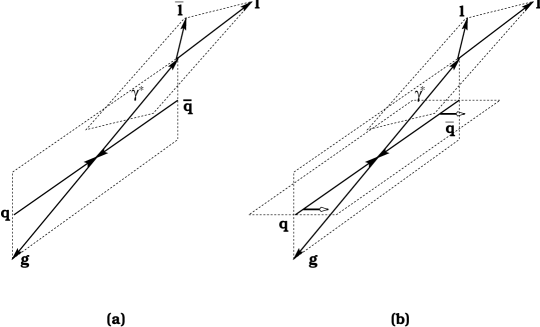
Figure 2: (a) the unpolarized QCD-annihilation process, (b) the case with transverse polarization.

For practical purposes we therefore made the crude but common assumption, that the transverse asymmetry of the QCD-annihilation graph equals the Drell-Yan one.

3 Sphinx tt

In order to estimate the transverse double spin asymmetry in the framework of our model we developped a new MC program for transversely polarized nucleon-nucleon scattering called Sphinx tt. It is based on the Lund Monte Carlo Pythia 5.6 [19] and is similar to Sphinx, a MC code for longitudinal polarized scattering.

Important features of Sphinx tt are:

• Polarization is described correctly in the initial state up to the hard partonic reaction. The spin orientations are not followed through the final states. String breaking and hadronization in general are assumed not to depend on the spin orientation.

• Two sets of polarized parton distributions are available by now. The parametrizations of $\Delta q(x,Q^{2})$ by Gehrmann/Stirling [12] and Bartelski/Tatur [13] are taken as transversity distributions at $Q_{0}^{2}=4{\rm GeV^{2}}$ and are evoluted according to the GLAP-equation (4). The implementation of other model parametrizations is easy.

• Transverse polarization is correctly taken care of in the initial state showering routine.

• The polarized partonic cross sections for high-$p_{T}$ jet production, prompt photon production and lepton pair production in the Drell-Yan model are available. $Z^{0}$ physics is not implemented yet.

• The majority of options of Pythia 5.6 is also available for Sphinx tt.

4 Results

Here we present the results of our MC calculations of $A^{TT}$ for the PHENIX detector at RHIC.

Our results are presented for $\sqrt{s}=50\,{\rm GeV}$ and an integrated luminosity of ${\cal L}=200{\rm pb}^{-1}$ as well as $\sqrt{s}=200\,{\rm GeV}$ and ${\cal L}=800{\rm pb}^{-1}$. This is equivalent to 230 days of beam time with 50% efficiency. The assumed integrated luminosity is larger by a factor of 2.5 compared to the standard value as quoted in [3, 4] but is necessary in order to detect an adequate number of events [5].

Taking into account this larger integrated luminosity as well as the expected Drell-Yan event rates for the STAR detector [4] the situation for this second detector is the same as presented below.

We assume that both endcaps will have a polar opening angle of $10^{\circ}-35^{\circ}$ with respect to the beam axis and will be able to measure myons with $1.1<y^{\mu}<2.5$. The central muon detectors are not very well suited for the measurement of $A^{TT}$ since they do not cover the full azimuth.

MC calculations [5] indicate competition from charm decay for $M_{\mu^{+}\mu^{-}}<4\,{\rm GeV}$ at $\sqrt{s}=50\,{\rm GeV}$ and $M_{\mu^{+}\mu^{-}}<5\,{\rm GeV}$ at $\sqrt{s}=200\,{\rm GeV}$ so that we set the minimum lepton pair mass accordingly. We did not set a cut to exclude the $\Upsilon$ production region at $8\,{\rm GeV}<M_{\mu^{+}\mu^{-}}<10\,{\rm GeV}$ because the cross section decreases exponentially with increasing $M_{\mu^{+}\mu^{-}}$ anyway.

Figure 3 shows the differential cross section ${\rm d}\sigma/{\rm d}q_{T}^{2}$ for both cm energies. The Drell-Yan graph obviously dominates lepton pair production for low $q_{T}$. The QCD Compton graph is the least important reaction in this region. In the high $q_{T}$ region we have the opposite situation. To enhance the Drell-Yan signal we therefore required $q_{T}<2\,{\rm GeV}$. This leads to an improvement of the $K^{DY}$-factor by $\Delta K^{DY}=-0.1$ for $\sqrt{s}=50\,{\rm GeV}$ and $\Delta K^{DY}=-0.3$ for $\sqrt{s}=200\,{\rm GeV}$ in our model. We multiplied the usual ${\cal O}(\alpha_{s})$-matrix elements of the hard partonic scattering with the corresponding form factors (11). Afterwards we fitted the width of the intrinsic momentum to the data at $\sqrt{s}=62\,{\rm GeV}$ taken from [20]. Unfortunately, we got $\langle k_{T}\rangle=800\,{\rm MeV}$ which is very high in comparison to DIS experiments. On the other hand we checked that the asymmetry does not depend on $\langle k_{T}\rangle$ for values smaller than 1 GeV. Our results are rather independent of the details. One should also note, that we switched off the general initial state showering routine because it is only suited for the large $q_{T}$ region and to avoid double counting. Bremsstrahlung effects are only taken into account by the QCD-annihilation and Compton process.

Figures 4 and 5 show the distribution of events in the plane of the Bjørken variables of the partons which participate in the hard interaction. Generally, the $x$-variables at $\sqrt{s}=200\,{\rm GeV}$ have smaller values as the ones at $\sqrt{s}=50\,{\rm GeV}$. In both cases, there is one region in the $x$-$x$-plane where most of the Drell-Yan type events are situated. These regions can be characterized by $0.3<x_{q}<0.7$ and $0.01<x_{\bar{q}}<0.04$ at $\sqrt{s}=50\,{\rm GeV}$, and $0.1<x_{q}<0.4$ and $0.002<x_{\bar{q}}<0.02$ at $\sqrt{s}=200\,{\rm GeV}$ respectively.

Figure 3: Distribution of the the transverse momentum of the virtual photon $q_{T}$ at $\sqrt{s}=50\,{\rm GeV}$ and $\sqrt{s}=200\,{\rm GeV}$. $q\bar{q}$ denotes the Drell-Yan graph, $q\bar{q}$ $B$ the QCD annihilation graph (B stands for Bremsstahlung).

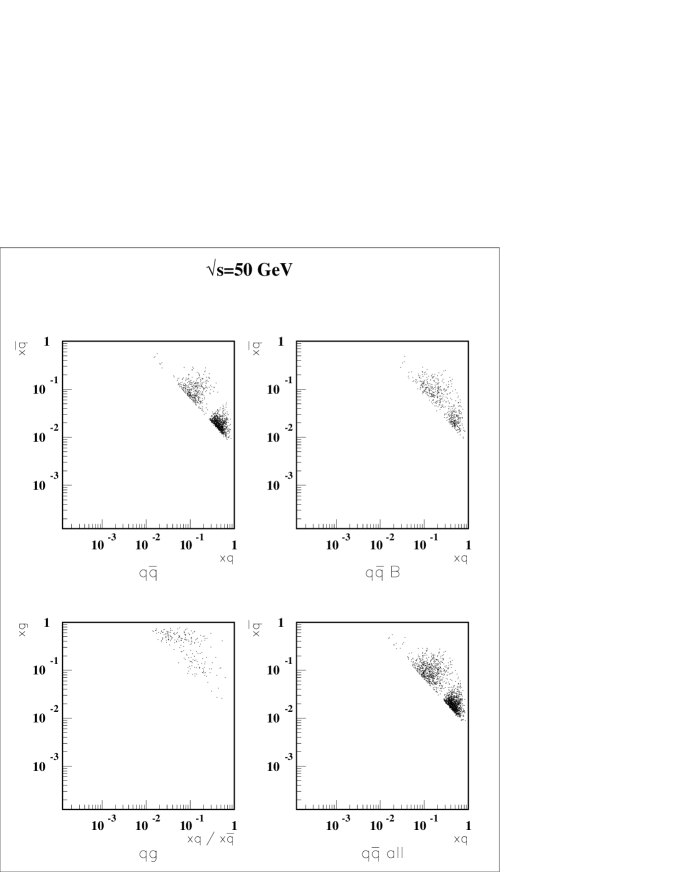
Figure 4: Event distribution in the plane of the Bjørken-$x$ of the partons that participate in the hard reaction at $\sqrt{s}=50$ GeV. $q\bar{q}$ denotes the Drell-Yan graph, $q\bar{q}$ $B$ the QCD annihilation graph.

Figure 5: Same as figure 4 for $\sqrt{s}=200$ GeV.

Fortunately, these ranges are also the ones, where the largest asymmetries are expected since the polaized parton distributions multiplied with $x$ have a maximum there. Therefore, it would be interesting to restrict the detected events to these regions. Furthermore, the exchange terms in equation (8) would disappear. In order to achieve this one has to calculate $x_{A/B}$ from the lepton momenta. Then one must decide which one of the incoming partons was the quark and which one was the antiquark. Since the majority of events fulfill $x_{q}>x_{\bar{q}}$ this criterium can be used very successfully for this purpose. In only 2%-10% of all cases the $x$-values are not assigned correctly.

Of course, it is not possible to reconstruct the $x$-values of the incoming partons of the QCD processes because the outgoing quark or gluon jet is not detected. Since the jet momentum is quite small in general we don’t make a big error by using the Drell-Yan formulas for the reconstruction of the Bjørken-$x$ also for the QCD processes.

Table 1 shows the event rates for the different cases. At $\sqrt{s}=200\,{\rm GeV}$ they are about ten to twenty times higher than for $\sqrt{s}=50\,{\rm GeV}$. This is mainly due to the fact that the unpolarized parton distributions rise steeply for smaller $x$. However, according to the shape of the transversity distributions for $\sqrt{s}=200\,{\rm GeV}$ one should expect a smaller $A^{TT}$. So we should try to minimize the statistical errors by integrating over all kinematical variables. The integration over the azimuth is performed as follows [11]

$$A^{TT}=\left\{\int\limits_{-\frac{\pi}{4}}^{\frac{\pi}{4}}-\int\limits_{\frac{\pi}{4}}^{\frac{3\pi}{4}}+\int\limits_{\frac{3\pi}{4}}^{\frac{5\pi}{4}}-\int\limits_{5\frac{\pi}{4}}^{7\frac{\pi}{4}}\right\}{\rm d}\phi\,A^{TT}(\phi)\quad.$$ (12)

For $\cos 2\phi$ this gives simply a factor of 4. According to our model the QCD annihilation graph carries the same asymmetry as the Drell-Yan graph which leads to

$$A^{TT}=\frac{N_{\rm DY}+N_{\rm annih.}}{N_{\rm DY}+N_{\rm annih.}+N_{\rm Compton}}A^{TT}_{\rm DY}\quad.$$ (13)

The statistical error of the asymmetry is $1/\sqrt{N}$ where $N$ denotes the total event rate.

Table 2 contains the results for the asymmetry together with the absolute statistical error. We can summarize them as follows:

• If $\delta q(x,4\,{\rm GeV}^{2})=\Delta q(x,4\,{\rm GeV}^{2})$ then $A^{TT}$ won’t be measurable at RHIC at $\sqrt{s}=50\,{\rm GeV}$ because the statistical error is approximately as large as the asymmetry itself.

• At $\sqrt{s}=200\,{\rm GeV}$ the relative statistical error is also very large, namely $60\%-80\%$. Therefore, it is very unlikely that the asymmetry can be measured as there will certainly be some unavoidable background and systematic error.

• The main reason for the predicted smallness of the asymmetry is the very small antiquark polarization which is of the order of 5% according to common parametrizations of parton distributions. By assuming a much larger sea polarization one gets larger asymmetries [10]. Consequently, there is a good chance that $A^{TT}$ can be measured at $\sqrt{s}=200\,{\rm GeV}$ if, e.g., $\delta\bar{q}(x,4\,{\rm GeV}^{2})=3\Delta\bar{q}(x,4\,{\rm GeV}^{2})$.

• It is crucial for the experiment that RHIC will be able run with the design luminosity in order to have enough events.

When we were writing this article we received [21] which describes a confinement model calculation of $\delta q(x,Q^{2})$. The authors also calculate $A^{TT}$ and their results are of the same order as the results presented in this paper.

Acknowledgements

We would like to thank Thomas Gehrmann for providing an evolution program for helicity distributions. We are also grateful to Torbjörn Sjöstrand for answering questions related to his program. This work was supported by DFG (Scha458/3) and BMBF.

PHENIX
subprocess	$\sqrt{s}=50\,{\rm GeV}$	$\sqrt{s}=200\,{\rm GeV}$
$q\bar{q}\rightarrow\mu^{+}\mu^{-}$	5236	70390
$q\bar{q}\rightarrow\mu^{+}\mu^{-}g$	2157	34720
$qg\rightarrow\mu^{+}\mu^{-}q$	637	10770
sum $N$	8030	115880
$K$-factor	1.5	1.6
PHENIX, $x$-$x$-Cuts
subprocess	$\sqrt{s}=50\,{\rm GeV}$	$\sqrt{s}=200\,{\rm GeV}$
$q\bar{q}\rightarrow\mu^{+}\mu^{-}$	3302	58020
$q\bar{q}\rightarrow\mu^{+}\mu^{-}g$	1027	27540
$qg\rightarrow\mu^{+}\mu^{-}q$	353	8740
sum $N$	4682	94300
$K$-factor	1.4	1.6

Table 1: Event rates.

PHENIX
parton distribution	$\sqrt{s}=50\,{\rm GeV}$	$\sqrt{s}=200\,{\rm GeV}$
Germann/Stirling	$1.00\%\pm 1.1\%$	$0.38\%\pm 0.30\%$
Bartelski/Tatur	$0.63\%\pm 1.1\%$	$0.51\%\pm 0.30\%$
PHENIX, $x$-$x$-Cuts
parton distribution	$\sqrt{s}=50\,{\rm GeV}$	$\sqrt{s}=200\,{\rm GeV}$
Germann/Stirling	$1.05\%\pm 1.4\%$	$0.45\%\pm 0.35\%$
Bartelski/Tatur	$1.70\%\pm 1.4\%$	$0.54\%\pm 0.35\%$

Table 2: Transverse double spin asymmetry $A^{TT}$ with absolute statistical error. The forseen polarization of beam and target at RHIC (70%) is already taken into account.

References

- [1] J.P. Ralston and D.E. Soper, Nucl. Phys. B152 (1979) 109.
- [2] X. Artru and M. Mekhfi, Z. Phys. C45 (1990) 669.
- [3] RHIC Spin Collaboration. Proposal on spin physics using the RHIC polarized collider. (1992)
- [4] STAR-RSC (RHIC Spin Collaboration), UPDATE. (1993)
- [5] The PHENIX/Spin Collaboration. Spin structure function physics with an upgraded PHENIX muon spectrometer. (1994)
- [6] X. Ji, Phys. Lett. B284 (1992) 137.
-
[7]
R.L. Jaffe and N. Saito, hep-ph/9604220 (1996),
submitted to Phys. Lett. B. - [8] R.L. Jaffe and X. Ji, Nucl. Phys. B375 (1992) 527.
- [9] H. He and X. Ji, Phys. Rev D52 (1995) 2960.
- [10] C. Bourrely and J. Soffer, Nucl. Phys. B423 (1994) 329.
- [11] J.L. Cortes, B. Pire and J.P. Ralston, Z. Phys. C55 (1992) 409.
- [12] T. Gehrmann and W.J. Stirling, hep-ph/9512406 (1995).
- [13] J. Bartelski and S. Tatur, hep-ph/9512393 (1995).
- [14] R.D. Field, Applications of perturbative QCD, Frontiers in Physics Volume No. 77, Addison-Wesley (1989), and references therein.
- [15] Y.L. Dokshitzer, D.I. Dyakonov and S.I. Troyan, Phys. Rep. 58 (1980) 269.
- [16] S.D. Ellis and W.J. Stirling, Phys. Rev. D23 (1981) 214.
-
[17]
J.C. Collins, D.E. Soper, G. Sterman,
Nucl. Phys. B250 (1985) 199.
G. Altarelli et al., Nucl. Phys. B246 (1984) 12. -
[18]
P. Chiapetta and M. Le Bellac, Z. Phys. C32 (1986)
521.
S. Gavin et al., in Hard Processes in Hadronic Interactions, edited by H. Satz and X.-N. Wang, Lawrence Berkeley Laboratory Report No. LBL-36984. -
[19]
T. Sjöstrand, Comp. Phys. Commun. 39 (1986) 347.
T. Sjöstrand and M. Bengtsson, Comp. Phys. Commun. 43 (1987) 367. - [20] D. Antreasyan et al., Phys. Rev. Lett. 47 (1981) 12.
- [21] V. Barone, T. Calarco and A. Drago, hep-ph/9605434 (1996).