Bayesian estimate of the effect of ${\rm B}^{0}\bar{\rm B}^{0}$ mixing measurements on the CKM matrix elements

Abstract

A method employing Bayesian statistics is used to incorporate recent experimental results on ${\rm B}^{0}_{\rm d}\bar{\rm B}^{0}_{\rm d}$ and ${\rm B}^{0}_{\rm s}\bar{\rm B}^{0}_{\rm s}$ mixing into a measurement of the Cabibbo-Kobayashi-Maskawa matrix elements with small theoretical uncertainties. The neutral B meson mixing results yield a slight improvement in the estimate of $|{\rm V}_{\rm td}|$. Prospects for improving the knowledge of the CKM matrix elements with measurements of ${\rm B}^{0}_{\rm s}\bar{\rm B}^{0}_{\rm s}$ mixing and the ${\rm K}^{+}\rightarrow\pi^{+}\nu\bar{\nu}$ branching ratio are considered.

The precise determination of the elements of the Cabibbo-Kobayashi-Maskawa (CKM) matrix [1] is one important goal of current experiments at BNL, CERN, CESR, FNAL, and SLAC and future experiments such as BaBar, Belle, CLEO-III, HERA-B, KTeV and LHC-B. Buras [2, 3] has pointed out that measurement of CP asymmetries in neutral B meson decays and the ${\rm K}_{\rm L}\rightarrow\pi^{\circ}\nu\bar{\nu}$ branching ratio can determine the CKM matrix with almost no theoretical uncertainties if ${\rm V}_{\rm us}$ is known. As yet, no measurements of these quantities exist. However, current experiments do provide information on two other useful measurements which are estimated to have ${\cal O}(10\%)$ theoretical uncertainties: the fractional ${\rm B}^{0}\bar{\rm B}^{0}$ mass difference and the ${\rm K}^{+}\rightarrow\pi^{+}\nu\bar{\nu}$ branching ratio.

1 ${\rm B}^{0}\bar{\rm B}^{0}$ mixing

In the Standard Model, mixing of neutral B mesons occurs via box diagrams dominated by internal top quark loops which allow the ratio of the CKM elements ${\rm V}_{\rm ts}/{\rm V}_{\rm td}$ to be determined from ${\rm B}^{0}_{\rm d}\bar{\rm B}^{0}_{\rm d}$ and ${\rm B}^{0}_{\rm s}\bar{\rm B}^{0}_{\rm s}$ mixing measurements [2, 4]:

$$\frac{\Delta m_{\rm s}}{\Delta m_{\rm d}}=\xi^{2}\frac{m_{\rm s}}{m_{\rm d}}\left|\frac{{\rm V}_{\rm ts}}{{\rm V}_{\rm td}}\right|^{2}$$ (1)

where $\Delta m_{\rm d}$ ($\Delta m_{\rm s}$) is the mass difference between the ${\rm B}^{0}_{\rm d}$ (${\rm B}^{0}_{\rm s}$) mass eigenstates, $m_{\rm s}$ ($m_{\rm d}$) is the ${\rm B}^{0}_{\rm d}$ (${\rm B}^{0}_{\rm s}$) mass and $\xi=1.16\pm 0.10$ [4] is the ratio of hadronic matrix elements for the ${\rm B}^{0}_{\rm s}$ and ${\rm B}^{0}_{\rm d}$ mesons and constitutes the theoretical uncertainty due to ${\rm SU}(3)_{\rm flavour}$ breaking effects. Currently, ${\rm B}^{0}_{\rm d}\bar{\rm B}^{0}_{\rm d}$ mixing is rather well measured, $\Delta m_{\rm d}=0.457\pm 0.019\ {\rm ps}^{-1}$ [5]; while experimental information from LEP on ${\rm B}^{0}_{\rm s}\bar{\rm B}^{0}_{\rm s}$ mixing indicates that $\Delta m_{\rm s}$ is at least ten times larger than $\Delta m_{\rm d}$ [6, 7, 8, 9, 10]. Although the LEP experiments are incapable of resolving values of $\Delta m_{\rm s}$ greater than $10\ {\rm ps}^{-1}$ due to their limited event samples and proper time resolution, we show that it is nonetheless possible to determine the additional constraints placed on the CKM matrix elements from the experimental information on B meson mixing using Bayes’ theorem. By way of demonstration, we first employ Bayes’ theorem to determine the allowed range of $\Delta m_{\rm s}$ given equation 1 and prior measurements of the magnitudes of CKM matrix elements [11].

For a proposition of interest $q$, prior knowledge $i$ and additional information $e$, Bayes’ theorem

$$P(q|i\wedge e)=P(q|i)\ P(e|i\wedge q)/P(e|i)$$ (2)

allows one to adjust the “prior probability” of $q$, $P(q|i)$, given the additional information $e$ [12]. The factor $P(e|i\wedge q)$ is called the “likelihood” and often factorizes further since $e$ is frequently the result of a sequence of statistically independent measurements and $P(e|i)$ can often be determined by normalization [13, 14, 15]. In our case, we use Bayes’ theorem to demonstrate how probability densities related to the CKM matrix are affected by recent ${\rm B}^{0}\bar{\rm B}^{0}$ mixing results and how these probabilities might further be affected by potential measurements of the ${\rm K}^{+}\rightarrow\pi^{+}\nu\bar{\nu}$ branching ratio.

Using the “standard” parameterization of the CKM matrix as recommended by the Particle Data Group (PDG) [11], the CKM matrix is determined by four angles $\Theta=(\theta_{12},\theta_{23},\theta_{13},\delta_{13})$. Assuming a uniform prior for $\Theta$ within $[0,\pi/2)^{3}\times[0,2\pi)$, the new probability density for $\Theta$ is

$$P(\Theta)=\prod_{i=1}^{6}g(v_{i},\mu_{i},\sigma_{i})$$ (3)

where $g(v,\mu,\sigma)$ is the Gaussian distribution and $v_{1},v_{2},\dots,v_{6}$ are the six quantities listed in Table 1

Matrix element	Magnitude
${\rm V}_{\rm ud}$	0.9736	$\pm$	0.0010
${\rm V}_{\rm us}$	0.2205	$\pm$	0.0018
${\rm V}_{\rm cd}$	0.224	$\pm$	0.016
${\rm V}_{\rm cs}$	1.01	$\pm$	0.18
${{\rm V}_{\rm ub}}/{{\rm V}_{\rm cb}}$	0.08	$\pm$	0.02
${\rm V}_{\rm cb}$	0.041	$\pm$	0.003

Table 1: Experimental determination of the magnitudes of six of the CKM matrix elements as compiled by the PDG [11].

expressed as functions on $[0,\pi/2)^{3}\times[0,2\pi)$ with independently measured values $\mu_{1},\mu_{2},\dots,\mu_{6}$ and corresponding variances $\sigma_{1}^{2},\sigma_{2}^{2},\dots,\sigma_{6}^{2}$. Once we have a probability density $\phi(\Theta)$ then the density $\psi(x)$ for any real function $f(\Theta)$,

$$\psi(x)=\frac{{\rm d}}{{\rm d}x}\int_{\Theta}{\rm d}\Theta\ \phi(\Theta)\ \lceil f(\Theta)\leq x\rceil\ ,$$ (4)

can be evaluated numerically [12, 16].

As an example of the method described above, consider the recent ALEPH study of the ${\rm B}^{0}_{\rm s}\bar{\rm B}^{0}_{\rm s}$ mass difference. As shown in Figure 1, the experimental likelihood function ${\cal L}(\Delta m_{\rm s})$ reflects the inability of the experiment to distinguish large values of $\Delta m_{\rm s}$ and only a lower limit on $\Delta m_{\rm s}$ is reported [8]. However, assuming equation 1 one can use the measurements in Table 1 together with measurements of $\Delta m_{\rm d}$ [5], the ${\rm B}^{0}$ meson masses [11] and a theoretical estimate of $\xi$ [4] as prior information in Bayes’ theorem to improve upon the ALEPH likelihood. Assuming that these measurements and theoretical estimates are independent and normally distributed, the prior probability density of $\Delta m_{\rm s}$ can be constructed from equation 4 given the constraints in Table 1 and is shown in Figure 1. There is a 95% probability that $\Delta m_{\rm s}>\ 5.8\ {\rm ps}^{-1}$ from the prior probability density alone. If the prior probability is combined with the ALEPH likelihood using Bayes’ theorem, then the lower limit improves to $7.5\ {\rm ps}^{-1}$ as shown in Figure 1.

Figure 1: The dotted curve shows the prior probability of $\Delta m_{\rm s}$ determined from the measurements in Table 1. The thin solid curve is ${\cal L}(\Delta m_{\rm s})$ the likelihood of $\Delta m_{\rm s}$ from the ALEPH experiment [8] and the thick solid curve is the overall probability of $\Delta m_{\rm s}$ determined using Bayes’ theorem. The normalization is arbitrary.

The influence of the ${\rm B}^{0}\bar{\rm B}^{0}$ mixing measurements on the CKM matrix elements can be determined if equation 1 is assumed. Given the ALEPH likelihood ${\cal L}(\Delta m_{\rm s})$ and assuming that $\Delta m_{\rm d}$, $\xi$, $m_{\rm s}$ and $m_{\rm d}$ are independent and Gaussian with means and variances as quoted above, then equation 4 can be used to determine the probability density for $|{\rm V}_{\rm ts}/{\rm V}_{\rm td}|$ or the likelihood $L(\Theta)$ of the ALEPH results given the CKM angles. Using this likelihood and the PDG prior $P(\Theta)$, the density $\psi_{ij}$ for the magnitude of CKM matrix element ${\rm V}_{ij}$ is determined by

$$\psi_{ij}(v)\propto\frac{{\rm d}}{{\rm d}v}\int_{\Theta}{\rm d}\Theta\ P(\Theta)\ L(\Theta)\ \lceil|{\rm V}_{ij}(\Theta)|\leq v\rceil$$ (5)

where the ${\rm V}_{ij}(\Theta)$ are the matrix elements expressed as a functions of the CKM angles. The resulting densities for the nine CKM elements, both with and without the ${\rm B}^{0}\bar{\rm B}^{0}$ mixing measurements, are shown in Figure 2. In the absence of ${\rm B}^{0}\bar{\rm B}^{0}$ mixing measurements, the 90% confidence limits on the matrix element magnitudes [17] are

$$\left(\begin{array}[]{ccc}{\rm V}_{\rm ud}&{\rm V}_{\rm us}&{\rm V}_{\rm ub}\\ {\rm V}_{\rm cd}&{\rm V}_{\rm cs}&{\rm V}_{\rm cb}\\ {\rm V}_{\rm td}&{\rm V}_{\rm ts}&{\rm V}_{\rm tb}\\ \end{array}\right)\sim{\left(\begin{array}[]{lcllcllcl}0.9745&\mbox{to}&0.9757&\ 0.219&\mbox{to}&0.224&\ 0.002&\mbox{to}&0.005\\ 0.219&\mbox{to}&0.224&\ 0.9736&\mbox{to}&0.9749&\ 0.036&\mbox{to}&0.046\\ 0.006&\mbox{to}&0.013&\ 0.035&\mbox{to}&0.045&\ 0.9989&\mbox{to}&0.9993\\ \end{array}\right)}\ .$$

There is good agreement between these results and the PDG [11] for all elements except for ${\rm V}_{\rm ts}$, which is due to their rounding procedure [18], and ${\rm V}_{\rm td}$, which is obviously non-Gaussian. The PDG [11, 18] and others [19, 20] use the method of least squares to calculate confidence levels which can lead to inaccurate results if the predicted distribution of the magnitude of a matrix element is non-Gaussian. The two-lobed structure of $|{\rm V}_{\rm td}|$ is due to the phase $\delta_{13}$ which is virtually unconstrained by the measurements of Table 1.

Figure 2: The probability density functions for the magnitudes of the nine CKM matrix elements. The solid curves show the probability densities determined with the PDG information in Table 1 alone; the dashed curves show the densities with the addition of the ${\rm B}^{0}\bar{\rm B}^{0}$ mixing results.

Only $|{\rm V}_{\rm td}|$ is significantly changed by the addition of the ${\rm B}^{0}\bar{\rm B}^{0}$ mixing information. As shown in Figure 2, the 90% confidence limits change from (0.0057 to 0.0131) to (0.0054 to 0.0121) as large values of $|{\rm V}_{\rm td}|$ are disfavoured by ${\cal L}(\Delta m_{\rm s})$ as shown in Figure 1.

2 The ${\rm K}^{+}\rightarrow\pi^{+}\nu\bar{\nu}$ branching ratio

A Bayesian estimate of the CKM matrix can also be constructed from ${\rm K}^{+}\rightarrow\pi^{+}\nu\bar{\nu}$ branching ratio measurements together with additional theoretical assumptions. The ${\rm K}^{+}\rightarrow\pi^{+}\nu_{\ell}\bar{\nu_{\ell}}$ branching ratio for a single lepton species $\ell$ is given by [21]

$$\mbox{Br}({\rm K}^{+}\rightarrow\pi^{+}\nu_{\ell}\bar{\nu_{\ell}})=\frac{\alpha^{2}\mbox{Br}({\rm K}^{+}\rightarrow\pi^{\circ}{\rm e}^{+}\nu_{\rm e})}{2\pi^{2}\sin^{4}{\theta}_{\rm w}}\times\frac{\left|{\rm V}^{\star}_{\rm cs}{\rm V}_{\rm cd}X^{\ell}_{NL}+{\rm V}^{\star}_{\rm ts}{\rm V}_{\rm td}X(x_{t})\right|^{2}}{\left|{\rm V}_{\rm us}\right|^{2}}\ ,$$ (6)

where $x_{t}\equiv m_{t}^{2}/m_{W}^{2}$. From Table 1 of reference [21], we assume $X^{\ell}_{NL}=(11.2\pm 1.0)\times 10^{-4}$ for $\ell=e,\mu$ and $X^{\ell}_{NL}=(7.6\pm 1.0)\times 10^{-4}$ for $\ell=\tau$ where the quoted errors are dominated by uncertainties in $\Lambda_{\overline{\rm MS}}$ and the charm quark mass. We use the approximation $X(x_{t})=0.65x_{t}^{0.575}$ which is accurate to better than 0.5% for $150\leq m_{t}\leq 190\ {\rm GeV}/c^{2}$ [3], and take $\alpha(m_{W})=1/128$, $\sin^{2}\theta_{\rm w}=0.23$, $m_{t}=180\pm 12\ {\rm GeV}/c^{2}$ [22], $m_{W}=80.32\pm 0.19\ {\rm GeV}/c^{2}$ and $\mbox{Br}({\rm K}^{+}\rightarrow\pi^{\circ}{\rm e}^{+}\nu_{\rm e})=4.82\pm 0.06\ \%$ [11].

The probability density of $B\equiv\mbox{Br}({\rm K}^{+}\rightarrow\pi^{+}\nu\bar{\nu})$, the branching ratio summed over $\ell={\rm e},\mu,\tau$, can be determined using the procedure of equation 4

$$\psi(B)=\frac{{\rm d}}{{\rm d}B}\int_{\Theta}{\rm d}\Theta\ P(\Theta)\ \lceil\beta(\Theta)<B\rceil$$ (7)

where $\Theta$ is now expanded to include $x_{t}$, $\mbox{Br}({\rm K}^{+}\rightarrow\pi^{\circ}{\rm e}^{+}\nu_{\rm e})$ and $X^{\ell}_{NL}$ as well as the six CKM measurements in Table 1. We assume that $x_{t}$, $\mbox{Br}({\rm K}^{+}\rightarrow\pi^{\circ}{\rm e}^{+}\nu_{\rm e})$ and $X^{\ell}_{NL}$ are independent and normally distributed about their central values but that the values of $X^{\ell}_{NL}$ are completely correlated for the three lepton species. With these assumptions and the constraints of Table 1, there is a 90% probability that $0.5\times 10^{-10}<\mbox{Br}({\rm K}^{+}\rightarrow\pi^{+}\nu\bar{\nu})<2.2\times 10^{-10}$ and the most probable value of the branching ratio is $0.8\times 10^{-10}$.

Figure 3: The dotted curve shows the probability density of the ${\rm K}^{+}\rightarrow\pi^{+}\nu\bar{\nu}$ branching ratio determined from the measurements in Table 1 and equations 6 and 7. The thin solid curve is the probability of $\mbox{Br}({\rm K}^{+}\rightarrow\pi^{+}\nu\bar{\nu})$ determined from BNL E787. The thick solid curve is the combined probability of $\mbox{Br}({\rm K}^{+}\rightarrow\pi^{+}\nu\bar{\nu})$. The normalization is arbitrary.

The current experimental upper limit at 90% confidence level of $2.4\times 10^{-9}$ [23] from BNL E787 is thus roughly an order of magnitude higher than the Standard Model prediction. From the recommended procedure for the calculation of confidence levels for Poisson processes with background [11], the probability density for $\mbox{Br}({\rm K}^{+}\rightarrow\pi^{+}\nu\bar{\nu})$ is $P_{e}(B)\propto\exp(-BAN_{{\rm K}^{+}})$ where $A=0.0027$ is the experimental acceptance and $N_{{\rm K}^{+}}=3.49\times 10^{11}$ is the number of stopped ${\rm K}^{+}$ [23]. The experimental result $P_{e}(B)$ is compared to the expected range from equation 7 in Figure 3. We also show the result of Bayes’ theorem for the combined probability for the ${\rm K}^{+}\rightarrow\pi^{+}\nu\bar{\nu}$ branching ratio. As expected the experimental result has no significant effect on the combined probability. The methods used in the paper should be useful in the near future as an upgraded version of BNL E787 is expected to be capable of observing the ${\rm K}^{+}\rightarrow\pi^{+}\nu\bar{\nu}$ decay assuming the Standard Model is correct [24]. In the following section we describe the possible effect of such a measurement on the unitarity triangle.

3 The unitarity triangle

The unitarity triangle is a convenient way to present the relations between the CKM matrix elements [11, 25]. The lengths of the sides of the triangle are given by $({\rm V}^{\star}_{\rm ub}{\rm V}_{\rm ud})/({\rm V}^{\star}_{\rm cb}{\rm V}_{\rm cd})$, $({\rm V}^{\star}_{\rm tb}{\rm V}_{\rm td})/({\rm V}^{\star}_{\rm cb}{\rm V}_{\rm cd})$ and 1. The side of unit length conventionally has endpoints at (0,0) and (1,0) in the complex plane so that the apex of the triangle is given by $(\rho,\eta)$.

A straightforward generalization of equation 4 allows us to calculate the probability density of $\rho$ and $\eta$, $\psi(\rho,\eta)$. Figure 4(a) shows the probability contours of $\psi(\rho,\eta)$ given the measurements in Table 1. The addition of the ${\rm B}^{0}\bar{\rm B}^{0}$ mixing information produces a slight modification of the contours as shown in Figure 4(b). Finally we show the contours given hypothetical measurements of $\Delta m_{\rm s}=12.5\pm 0.5\ {\rm ps}^{-1}$ and $\mbox{Br}({\rm K}^{+}\rightarrow\pi^{+}\nu\bar{\nu})=(1.0\ \pm\ 0.1)\times 10^{-10}$ in Figure 4(c). With these two measurements, there would be a 90% probability that $0.0077<|{\rm V}_{\rm td}|<0.0106$ and the most probable value of $|{\rm V}_{\rm td}|$ would be $0.0088$. As seen in Figure 4(c), it would be possible to confirm the prediction of CP violation ($\eta\not=0$) by the Standard Model at the 95% confidence level with these two particular measurements.

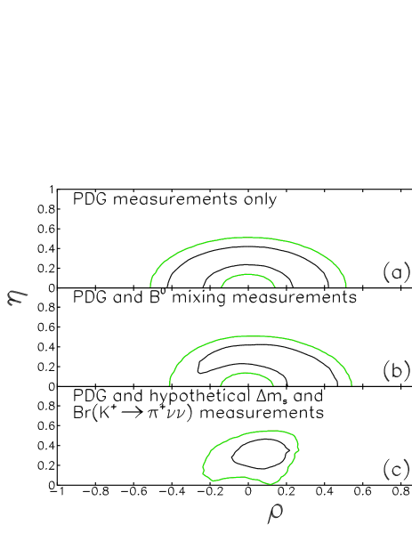
Figure 4: The 68.3% (dark) and 95.5% (light) probability contours for the apex of the unitarity triangle determined using (a) the measurements listed in Table 1 only, (b) the ${\rm B}^{0}\bar{\rm B}^{0}$ mixing results and Table 1, and (c) Table 1 and hypothetical measurements of $\Delta m_{\rm s}=12.5\pm 0.5\ {\rm ps}^{-1}$ and $\mbox{Br}({\rm K}^{+}\rightarrow\pi^{+}\nu\bar{\nu})=(1.0\pm 0.1)\times 10^{-10}$. A non-zero $\eta$ would confirm CP violation as predicted by the Standard Model.

4 Conclusions

Using Bayes’ theorem, recent measurements of ${\rm B}^{0}\bar{\rm B}^{0}$ mixing are used to improve upon current estimates of the CKM matrix elements with minimal theoretical uncertainty. Only $|{\rm V}_{\rm td}|$ is significantly affected by these results. The impact of current and potential measurements of ${\rm B}^{0}\bar{\rm B}^{0}$ mixing and the ${\rm K}^{+}\rightarrow\pi^{+}\nu\bar{\nu}$ branching ratio on the individual CKM matrix elements and the CKM unitarity triangle is also examined.

This work was supported by US Department of Energy contracts DE-FG05-92ER40742 and DE-FC05-85ER250000.

References

• [1] N. Cabibbo, Phys. Rev. Lett. 10 (1963) 531;
M. Kobayashi and T. Maskawa, Prog. Theor. Phys. 49 (1973) 652.
• [2] A.J. Buras, “Towards precise determinations of the CKM matrix without hadronic uncertainties”, Invited talk at the 27th International Conference on High Energy Physics, Glasgow, Scotland, 20-27 July, 1994. Proceedings, High Energy Physics, Vol. 2 1307-1310.
• [3] A.J. Buras, Phys. Lett B333 (1994) 476.
• [4] A. Ali and D. London, Z. Phys. C65 (1995) 431.
• [5] S.L. Wu, “Recent results on B meson oscillations”, Invited talk at the XVII International Symposium on Lepton-Photon Interactions, Beijing, China August 1995, hep-ex/9602003.
• [6] D. Buskulic et al., ALEPH Collaboration, Phys. Lett. B322 (1994) 441;
ALEPH Collaboration, “Measurement of the ${\rm B}^{0}_{\rm d}\bar{\rm B}^{0}_{\rm d}$ oscillation frequency”, submitted to the International Europhysics Conference on High Energy Physics, Brussels, Belgium, 1995, reference eps0409.
• [7] D. Buskulic et al., ALEPH Collaboration, Phys. Lett. B356 (1995) 409.
• [8] “Study of the ${{\rm B}^{0}_{\rm s}{\bar{\rm B}}^{0}_{\rm s}}$ oscillation frequency using D${}_{\rm s}^{-}{\ell}^{+}$ combinations in Z decays”, ALEPH Collaboration, D. Buskulic et.al., CERN-PPE 96/30, to be published in Phys. Lett. B.
• [9] DELPHI Collaboration, “Improved measurement of the oscillation frequencies of B0 mesons”, submitted to the International Europhysics Conference on High Energy Physics, Brussels, Belgium, 1995, reference eps0568.
• [10] R. Akers et al., OPAL Collaboration, Z. Phys. C66 (1995) 555;
OPAL Collaboration, “A study of B meson oscillation using inclusive lepton events”, submitted to the International Symposium on Lepton-Photon Interactions, Beijing, China, (1995).
• [11] R.M. Barnett et. al., Particle Data Group, Phys. Rev. D54 (1996) 1.
• [12] For propositions $a,b$, “$a\wedge b$” denotes $a\ {\bf and}\ b$ and $\lceil\ a\ \rceil$ denotes the function 1 if $a$ is $true$ and 0 if $a$ is $false$.
• [13] E.T. Jaynes, “Confidence intervals vs Bayesian intervals”, Foundations of Probability Theory, Statistical Inference, and Statistical Theories of Science, Vol. II, W.L. Harper and C.A. Hooker, eds., D. Reidel Publishing Co., Dordecht, Holland, 1976. See also: Probability Theory - The Logic of Science at URL http://omega.albany.edu:8008/JaynesBook.html.
• [14] E.T. Jaynes, “Prior information and ambiguity in inverse problems”, in SIAM-AMS Proceedings, Vol. 14, American Mathematical Society, 1984, pp. 151-166.
• [15] R.T. Cox, Am. J. Phys. 14, 1(1946).
• [16] G. Peter Lepage, “VEGAS: an adaptive multidimensional integration program”, CLNS-80/447, 1980.
• [17] For a probability density function $\phi(x)$, we quote the central confidence interval $[a,b]$ of probability $p$ as defined by $\int_{-\infty}^{a}{\rm d}x\ \phi(x)=\frac{1-p}{2}=\int^{\infty}_{b}{\rm d}x\ \phi(x)$. See also: W.T. Eadie, D. Dryard, F.E. James, M. Roos and B. Sadoulet, Statistical Methods in Experimental Physics, North-Holland Publishing Co., Amsterdam, Holland, 1971.
• [18] Burkhard Renk, private communication.
• [19] M. Schmidtler and K.R. Schubert, Z. Phys. C53 (1992) 347.
• [20] W.-S. Choong and D. Silverman, Phys. Rev. D49 (1994) 1649.
• [21] G. Buchalla and A.J. Buras, Nucl. Phys. B412 (1994) 106.
• [22] S. Abachi et. al., D$\emptyset$ Collaboration, Phys. Rev. Lett. 74 (1995) 2632;
F. Abe et. al., CDF Collaboration, Phys. Rev. Lett. 74 (1995) 2626.
• [23] S. Adler et. al., BNL E787, Phys. Rev. Lett. 76 (1996) 1421.
• [24] Robert McPherson, private communication.
• [25] L.-L. Chau and W.-Y. Keung, Phys. Rev. Lett. 53 (1984) 1802.