ABSTRACT

We calculate the $U(1)$ continuum gauge coupling using the values of action parameters coinciding with the multiple point. This is a point in the phase diagram of a lattice gauge theory where a maximum number of phases convene. We obtain for the running inverse finestructure constant the values $\alpha_{1}^{-1}=56\pm 5$ and $\alpha_{1}^{-1}=99\pm 5$ at respectively the Planck scale and the $M_{Z}$ scale. The gauge group underlying the phase diagram in which we seek multiple point parameters is what we call the Anti Grand Unified Theory (AGUT) gauge group $SMG^{3}$ which is the Cartesian product of 3 standard model groups (SMGs). There is one SMG factor for each of the $N_{gen}=3$ generations of quarks and leptons. In our model, this gauge group $SMG^{3}$ is the predecessor to the usual standard model group. The latter arises as the diagonal subgroup surviving the Planck scale breakdown of $SMG^{3}$. This breakdown leads to a weakening of the $U(1)$ coupling by a $N_{gen}$-related factor. For $N_{gen}=3$, this factor would be $N_{gen}(N_{gen}+1)/2=6$ if phase transitions between all the phases convening at the multiple point were purely second order. The factor $N_{gen}(N_{gen}+1)/2=6$ corresponds to the six gauge invariant combinations of the $N_{gen}=3$ different $U(1)$s that give action contributions that are second order in $F_{\mu\nu}$. The factor analogous to this $N_{gen}(N_{gen}+1)/2=6$ in the case of the earlier considered non-Abelian couplings reduced to the factor $N_{gen}=3$ because action terms quadratic in $F_{\mu\nu}$ that arise as contributions from two different of the $N_{gen}=3$ SMG factors of $SMG^{3}$ are forbidden by the requirement of gauge symmetry.

Actually we seek the multiple point in the phase diagram of the gauge group $U(1)^{3}$ as a simplifying approximation to the desired gauge group $SMG^{3}$. The most important correction obtained from using multiple point parameter values (in a multi-parameter phase diagram instead of the single critical parameter value obtained say in the 1-dimensional phase diagram of a Wilson action) comes from the effect of including the influence of also having at this point phases confined solely w.r.t. discrete subgroups. In particular, what matters is that the degree of first orderness is taken into account in making the transition from these latter phases at the multiple point to the totally Coulomb-like phase. This gives rise to a discontinuity $\Delta\gamma_{eff}$ in an effective parameter $\gamma_{eff}$. Using our calculated value of the quantity $\Delta\gamma_{eff}$, we calculate the above-mentioned weakening factor to be more like 6.5 instead of the $N_{gen}(N_{gen}+1)/2=6$ as would be the case if all multiple point transitions were purely second order. Using this same $\Delta\gamma_{eff}$, we also calculate the continuum $U(1)$ coupling corresponding to the multiple point of a single $U(1)$. The product of this latter and the weakening factor of about 6.5 yields our Planck scale prediction for the continuum $U(1)$ gauge coupling: i.e., the multiple point critical coupling of the diagonal subgroup of $U(1)^{3}\in SMG^{3}$. Combining this with the results of earlier work on the non-Abelian gauge couplings leads to our prediction of $\alpha^{-1}=136._{8}\pm 9$ as the value for the fine-structure constant at low energies.

1 Introduction

Over a period of a number of years we have put forth[1, 2, 3, 4, 5, 6] the observation that the actual values of the standard model running coupling constants $\alpha_{i}(\mu)$ $(i\in\{U(1),SU(2),SU(3)\})$ at the Planck energy scale $\mu_{Pl}$ (i.e., experimental values extrapolated to the Planck scale using the assumption of a minimal standard model) depart from critical values for a standard model group lattice gauge theory by a factor that is close to three for the non-Abelian $SU(2)$ and $SU(3)$ couplings (strictly speaking, this applies rather to the simple groups $SU(2)/\mbox{\bf{Z}}_{2}$ and $SU(3)/\mbox{\bf{Z}}_{3}$ having the same Lie algebra as $SU(2)$ and $SU(3)$).

We proposed the so-called $AGUT$ gauge group at the “fundamental scale” $\mu_{Pl}$ consisting of the 3-fold Cartesian product of the standard model group (sometimes referred to by use of the acronym “$AGUT$”: Anti Grand Unified Theory):

$$SMG\times SMG\times SMG\stackrel{{\scriptstyle def}}{{=}}SMG^{3}.$$ (1)

as way of “explaining” the phenomenologically indicated factors of three. Here we are anticipating that these factors, up to minor, controllable corrections, really have the integer value three.

Actually, rather than taking the $SMG$ as the group $U(1)\times SU(2)\times SU(3)$, we use instead a different group denoted as $S(U(2)\times U(3))$. However, both groups have the same Lie algebra. From the beginning we have assumed that the number of Cartesian product factors of the $SMG$ in $SMG^{3}$ is equal to the number of quark and lepton generations $N_{gen}$ so that each generation has its own set of gauge degrees of freedom. In our early[6, 7, 8] work in this series, we used a fitting procedure that lead us to conclude that the number of generations $N_{gen}$ was 3 prior to the subsequent experimental confirmation of $N_{gen}=3$ in $LEP$ measurements. We might therefore claim to have predicted the number of generations as being three at a time when the number $N_{gen}$ was essentially unknown except from notoriously unreliable cosmological fits.

In our more recent work[2, 1, 3, 4] we venture what can be said to be a more eloquent formulation in which fitting parameters are avoided and a number of assumptions made previously are essentially reduced to the postulate that the running gauge couplings at the Planck scale assume multiple point critical values. The multiple point is defined as the point in plaquette action parameter space where the largest possible number of “phases” in a lattice gauge theory come together. This requires that the functional form of the plaquette action - as defined by the parameters that span the space in which we seek the multiple point - is sufficiently general to “provoke” all the “phases” that we seek to bring together at the multiple point.

Although we suspect that it may be possible to avoid the assumption of a fundamental, truly existing lattice , this assumption is the most straight forward approach to our model.

To get an idea of what is meant by the “phases” that convene at the multiple point, recall first that the gauge field $U(\mbox{\begin{picture}(4.15,10.0)\put(0.0,3.0){\circle*{2.0}} \put(0.0,2.75){\line(1,0){7.0}} \put(7.3,3.0){\circle*{2.0}}\mbox{ } \end{picture} })$ assigns an element of the gauge group $G$ to each link of the lattice: $U:\{\;\mbox{\begin{picture}(4.15,10.0)\put(0.0,3.0){\circle*{2.0}} \put(0.0,2.75){\line(1,0){7.0}} \put(7.3,3.0){\circle*{2.0}}\mbox{ } \end{picture} }^{\!\!\!\!\!\!\!x^{\mu}\;\;y^{\mu}}\}\rightarrow G$. For complicated gauge groups such as $SMG$ and $SMG^{3}$ having many subgroups (and invariant subgroups), it will be seen that degrees of freedom corresponding to different subgroups can have qualitatively different fluctuation patterns. In other words, the region of action parameter space corresponding to some “phase” corresponds, in general, to different fluctuation patterns along different subgroups. The various phases can be classified using the different subgroups of the gauge group. We shall see that a “phase” is labelled by a subgroup $K\subseteq SMG^{N_{gen}}$ and an invariant subgroup $H\lhd K$. These labels $(K,H)$ characterise a possible qualitative physical behaviour of the vacuum that could be perceived using a small band of wavelengths at a given energy scale (the Planck scale in this case). More precisely, the elaboration of the “phases” $(K,H)$ is a classification of qualitatively different physical behaviours of the vacuum of a lattice gauge theory at the lattice scale[9] according to whether or not there is spontaneous breakdown of the gauge symmetry remaining after making a choice of gauge that we here take to be the (latticized) Lorentz gauge condition (i.e., for all sites $\mbox{\begin{picture}(4.15,4.0)\put(2.0,2.0){\circle*{2.0}} \end{picture} }^{\!\!\!x^{\mu}}$, $\prod_{\;\;\;\mbox{\begin{picture}(4.15,10.0)\put(0.0,3.0){\circle*{2.0}} \put(0.0,2.75){\line(1,0){7.0}} \put(7.3,3.0){\circle*{2.0}}\mbox{ } \end{picture} }^{\!\!\!\!\!\!\!x^{\mu}\;\;}\;\;\;\mbox{\tiny at }\mbox{\begin{picture}(4.15,4.0)\put(2.0,2.0){\circle*{2.0}} \end{picture} }^{\!\!\!x^{\mu}}}U\mbox{( $\;\mbox{\begin{picture}(4.15,10.0)\put(0.0,3.0){\circle*{2.0}} \put(0.0,2.75){\line(1,0){7.0}} \put(7.3,3.0){\circle*{2.0}}\mbox{ } \end{picture} }^{\!\!\!\!\!\!\!x^{\mu}\;\;}$ )}=1$ where $\;\;\;\mbox{\begin{picture}(4.15,10.0)\put(0.0,3.0){\circle*{2.0}} \put(0.0,2.75){\line(1,0){7.0}} \put(7.3,3.0){\circle*{2.0}}\mbox{ } \end{picture} }^{\!\!\!\!\!\!\!x^{\mu}\;\;}\;\;\;\mbox{\tiny at }\mbox{\begin{picture}(4.15,4.0)\put(2.0,2.0){\circle*{2.0}} \end{picture} }^{\!\!\!x^{\mu}}$ denotes a link that emanate from $\mbox{\begin{picture}(4.15,4.0)\put(2.0,2.0){\circle*{2.0}} \end{picture} }^{\!\!\!x^{\mu}}$ ). This choice of gauge still allows the freedom to perform gauge transformations of the types $\Lambda_{Const.}(x)=e^{i\alpha^{a}t^{a}}$ and $\Lambda_{Linear}(x)=e^{i\alpha^{a}t^{a}a_{\mu}x^{\mu}}$ respectively having constant and linear gauge functions ($a$ is a “colour” index labelling components $\alpha^{a}$ and generators $t^{a}$ of the Lie algebra). Such gauge transformations are used in defining the “phases” $(K,H)$ of the vacuum. Here we use the idea of different degrees of spontaneous symmetry breaking as a way to classify phases. This sort of classification can depend on the scale at which the classification is made. To illustrate this, one can think of two different regions of action parameter space with which are associated different finite correlation lengths. If the physics of these two regions is probed at a scale intermediate to these two correlation lengths, it would appear as though one region were Coulomb-like and the other confining and therefore separated by a phase transition. However, an examination of these regions at a length scale short compared to both correlation lengths would not detect a phase transition because both regions would appear to be in a Coulomb-like phase. The phase transition would also go undetected if the physics of the two regions were probed at a length scale large compared to both correlation lengths because both regions would appear to be confining. This situation is well known (e.g., in non-Abelian groups): a transition between Coulomb-like and confining lattice scale phases - “lattice artifacts” - often “disappear” in going to long wavelengths because phase diagram regions on both sides of the lattice scale transition are perceived as being in confinement at long distances.

Although we classify these phases with reference to a certain scale of wavelengths, there are nevertheless typically true first order phase transitions that are sharply defined in a specific regularization. In our model, we take the view that the regulator is not arbitrary but rather an ontological attribute of fundamental scale physics. From this point of view, “lattice artifact” phases assume a role that has physical implications.

In Section 2 we state the principle of multiple point criticality first in terms of the “lattice artifact” phases of a lattice gauge theory and then, in a more general context, as the prototype of a fine-tuning mechanism that results from arguing that even randomly fixed values of some extensive quantities of some sort or another will with a finite probability enforce the coexistence of two or more phases if the transition between these phases are first order. The presence of two or more phases separated by first order transitions fine-tunes “coupling constants” in a manner reminiscent of the way that temperature and pressure are fine-tuned at the triple point of water. Section 3 considers problems encountered in implementing the principle of multiple point criticality in the case of $U(1)$ as compared to the simpler case of the non-Abelian subgroups of the standard model. These problems, related to the “Abelian-ness” of $U(1)$ include the problem of charge normalisation and also the interactions between the $N_{gen}=3$ replicas of $U(1)$ in the AGUT gauge group $SMG^{3}$. In the roughest approximation, these interactions result in a weakening of the diagonal subgroup coupling of $U(1)^{3}\in SMG^{3}$ by a factor of $N_{gen}(N_{gen}+1)/2=6$ instead of the weakening factor $N_{gen}=3$ that applies to the non-Abelian subgroups (for which such interactions are not gauge invariant). Section 4 deals with approximate methods for constructing phase diagrams for the gauge group $U(1)^{3}$ in which we can seek out multiple point parameter values. After a brief discussion of how phases at the scale of a lattice regulator are classified, we develop a formalism that allows us to seek multiple point parameter values by adjusting the metric (which amounts to adjusting the parameters of a Manton action) in a $N_{gen}$-dimensional space upon which is superimposed an hexagonally symmetric lattice of points identified with the identity of $U(1)^{3}$. The hexagonal symmetry takes into account the allowed interactions between the $N_{gen}=3$ $U(1)$ factors of $U(1)^{3}$. Using this formalism, two approximative methods of determining phase boundaries are developed: the independent monopole and the group volume approximations. These describe respectively phase transitions that are purely second order and strongly first order. Calculations are done in Section 5 where we interpolate between the extreme situations described by the group volume and independent monopole approximations. This interpolation is done by calculating the discontinuity $\Delta\gamma_{eff}$ in an effective coupling $\gamma_{eff}$ at the multiple point. The dominant contributions to $\Delta\gamma_{eff}$ are due to multiple point transitions between phases that differ by the confinement of discrete subgroups (rather than continuous subgroups). The calculated $\Delta\gamma_{eff}$ reflects the degree of first-orderness of these transitions. As a result of including this effect the weakening factor $N_{gen}(N_{gen}+1)/2=6$ increases to about 6.5. The quantity $\Delta\gamma_{eff}$ is also used (together with $\gamma_{eff}$) to calculate the continuum $U(1)$ coupling corresponding to the multiple point of a single $U(1)$ which is then divided by the square root of the weakening factor of about 6.5 to get our prediction for the value of the running $U(1)$ coupling at the Planck scale. We also give values of the $U(1)$ coupling at scale of $M_{Z}$ obtained using the assumption of the minimal standard model in doing the renormalization group extrapolation. We present a number of values reflecting various approximations. In presenting what we take to be the “most correct” result, we compute the uncertainty from the deviations arising from plausibly correct ways of making distinctions in how different discrete subgroups enter into the calculation of $\Delta\gamma_{eff}$. The paper ends with concluding remarks in Section 6.

2 The Model

2.1 Multiple Point Criticality

The $SMG$ and, to an even greater extent, the $AGUT$ gauge group $SMG^{3}$ are non-simple groups with many subgroups and invariant subgroups. As already mentioned above, there can be a distinct “phase” for each pair of subgroups $(K,H)$ such that $H\triangleleft K\subseteq SMG^{3}$ (the symbol“$\triangleleft$ ” means “invariant subgroup of”). Such “phases”, which are often referred to as lattice artifacts, characterise qualitative physical behaviours that can be distinguished at least at the scale of the lattice. The principle of multiple point criticality states that Nature seeks out a point (the multiple point) in the phase diagram of a lattice gauge theory (with gauge group $SMG^{3}$) where a maximum number of “phases” come together.

2.1.1 Multiple point criticality: a very general model for fine-tuning

While the validity of the multiple point criticality principle is, in the context of our model, suggested alone on phenomenological grounds, we suspect that in a more general context, this principle is the consequence of having fixed amounts of some - presumably a multitude of - extensive quantities in spacetime . Universally fixed amounts of these extensive quantities could quite plausibly impose constraints that can only be fulfilled by having the coexistence of several “phases”. The idea is that having fixed amounts of certain extensive quantities can enforce the coexistence of several phases and in so doing place constraints on intensive parameters (e.g., gauge couplings, the cosmological constant). This idea provides a possible explanation for the “fine-tuned” parameters found in Nature in a manner suggested by the following analogous situation. Think of an equilibrium system enclosed by a container within which there is water in all three phases: solid, liquid, and ice. If the container is rigid and also impenetrable to heat and water molecules, we have accordingly fixed amounts of the extensive quantities: energy, mole number of water, and volume. There is a whole range of values at which the average energy and average volume per molecule can be fixed such that the system is forced to maintain the presence of all three phases. The enforced coexistence of all three phases in the presence of rapid changes in energy (i.e., non-vanishing heats of fusion, sublimation or vaporisation) as a function of the intensive parameters temperature and pressure in going from one phase to another “fine-tunes” the values of these parameters to those of the triple point of water. This mechanism provides a mechanism for fine-tuning that is effective if the transition is first order so that there is a “hop” in energy (and entropy) as a function of e.g. temperature.

Having (globally) fixed amounts of extensive quantities corresponding to 4-dimensional path integrals implies, strictly speaking, that locality is broken. This could, for example, come about in statistical mechanics where the use of a microcanonical ensemble can, taken in a stringent sense, imply correlations over long distances. This last remark is to be understood in the following way: having knowledge of the fixed amounts of the extensive quantities and thereby the amounts of the various phases means that if we at some place find a given phase, we can immediately conclude that the probability for finding more of this phase elsewhere - even at far-removed places - is smaller.

However it has been shown [9] that the non-locality introduced in this manner is harmless insofar as it does not lead to experimentally observable violations of locality. This mild form of non-locality is manifested in spacetime in a completely homogeneous way and it is tolerable physically precisely because its omni-presence in spacetime allows it to be incorporated into universal intensive constants of Nature (coupling constants).

The idea[10, 11, 12] of fixed extensive quantities is suggested by examining the limitations on the form that a nonlocal action can have if it is required to be diffeomorphism invariant (as a natural extension of translational invariance in general relativity). A simple but, for the purposes of long wavelength limits, very general form for a nonlocal Lagrangian action[9] is a general function $S_{nl}(I_{1},I_{2},\cdots)$ of all the (diffeomorphism invariant) spacetime integrals

$$I_{j}\stackrel{{\scriptstyle def}}{{=}}\int\sqrt{g(x)}{\cal L}_{j}(\phi(x),\partial_{\mu}\phi(x))d^{4}x$$ (4)

where $g=|\det g_{\mu\nu}|$ and the index $j$ enumerates the possible local field functions ${\cal L}_{j}$ with symmetry properties allowing them as Lagrange density terms.

With this functional form of the action, it follows that there are fixed amounts (i.e., given alone by the form of the action $S_{nl}$) of extensive quantities $I_{j}$ equal to the values of these spacetime integrals $I_{j}$ which yield the extremum of $S_{nl}$ (classical approximation). The action terms $S_{nl}$ consist typically of nonlinear (and thereby nonlocal) functions of the reparameterization invariant integrals $I_{j}$. Such action terms $S_{nl}(\{I_{j}\})$ are then also reparameterization invariant and the functional derivatives of $S_{nl}$ w.r.t. the fields become essentially local in the sense that these derivatives have the same value as seen from all spacetime points. Non-locality that comes about in this phenomenologically un-offensive way is manifested as the omnipresent values of constants of Nature. It is interesting that the potential paradoxes inherent to a theory with non-locality (e.g., of the “matricide” type naively encountered in “time machines”) are averted by a unique compromise that exists generically with a finite probability. We can show[13] that this unique solution coincides with multiple point values of intensive quantities such as fine structure constants and the cosmological constant.

2.2 AGUT with the gauge group $SMG^{3}$ and its breakdown to the $SMG$

In the context of our model, the experimental values for the fine-structure constants for the weak $SU(2)$ and the $QCD$ $SU(3)$ (after extrapolation to the Planck scale) are, to within the bounds of our uncertainty in making continuum corrections and other uncertainties, three times weaker than the values corresponding to the triple point in an $SU(N)$ lattice gauge theory using results from Monte Carlo calculations[14, 15, 16, 17]. However, to claim that the weakening factor has the integer value three would be somewhat presumptuous at this stage because of our lack of complete understanding of possible singularities (at the multiple point) in the continuum coupling as a function of bare parameters. Our concern comes about because such singularities are observed in numerical simulations[18] of the $U(1)$ continuum coupling. There is the hope that the effect of analogous singularities on the values of the non-Abelian couplings would be mitigated by a factor $1/(N^{2}-1)$ for $SU(N)$ groups. This is suggested if it is assumed that monopoles are responsible for the singularity. If however, we proceed using the assumption of an integer 3 relationship, we propose as an explanation that the gauge subgroups $SU(2)$, $SU(3)$, and $U(1)$ are embedded as the diagonal subgroup in the $AGUT$ gauge group $SMG^{3}$. The $AGUT$ gauge group $SMG^{3}$ is the Cartesian product of $N_{gen}=3$ group factors $SMG$:

$$SMG^{3}\stackrel{{\scriptstyle def}}{{=}}(U(1)_{Peter}\times U(1)_{Paul}\times U(1)_{Maria})\times$$ (5)

$$\times(SU(2)_{Peter}\times SU(2)_{Paul}\times SU(2)_{Maria})\times(SU(3)_{Peter}\times SU(3)_{Paul}\times SU(3)_{Maria})$$

where the labels “$Peter"$, “$Paul"$, $etc.$ distinguish the $N_{gen}$ different isomorphic Cartesian product group $SMG$ factors. The quantity $N_{gen}$ denotes the number of quark and lepton generations and is taken as 3 in accord with experimental results.

Before dealing with the gauge subgroup of primary interest in the present article - namely $U(1)^{3}\subseteq SMG^{3}$ - it will be instructive to first consider the subgroup $SU(N)^{3}\subseteq SMG^{3}$ $(N=2,3)$. In our proposal, the $SU(2)$ and $SU(3)$ subgroups of the standard model group are realized as the diagonal subgroups of $SU(2)^{N_{gen}}$ and $SU(3)^{N_{gen}}$ respectively. The breakdown of the non-Abelian Cartesian product subgroups of the $AGUT$ gauge group $SMG^{3}$ to the diagonal subgroups $SU(2)_{diag}$ and $SU(3)_{diag}$ can come about by different mechanisms. One breakdown mechanism, referred to as “confusion” [19, 20, 9, 21], comes about due to ambiguities that arise under group automorphic symmetry operations. Such ambiguities are also present in gauge groups with duplicated factors in Cartesian product groups such as our $AGUT$ with gauge group $SMG^{N_{gen}}$. Having the confusion mechanism of breakdown provides therefore a natural explanation for having a diagonal pattern of symmetry breakdown; i.e., gauge group couplings corresponding to groups embedded diagonally in groups with repeated Cartesian product factors.

The diagonal subgroup by definition consists of the elements $(U_{Peter},U_{Paul},\cdots,U_{N_{gen}})$ of $SU(N)^{N_{gen}}$ having identical excitations of the “$Peter$”, “$Paul$”, $etc.$ Cartesian product factors: $U_{Peter}=U_{Paul}=\cdots=U_{N_{gen}}=U_{common}$. That is,

$$SU(N)\stackrel{{\scriptstyle-}}{{\simeq}}SU(N)_{diag}^{N_{gen}}\stackrel{{\scriptstyle def}}{{=}}$$ (6)

$$\{(U_{common},U_{common},\cdots,U_{common})|U_{common}\in SU(N)\}\subseteq$$

$$\subseteq\underbrace{SU(N)\times SU(N)\times\cdots\times SU(N)}_{\tiny N_{gen}\mbox{ factors}}\;\;\;(N=2,3).$$

When the gauge group is realized in this way, it is readily shown that the inverse fine-structure constant for $SU(N)_{diag}^{N_{gen}}$ is additive in those of the $N_{gen}$ Cartesian product group factors of $SU(N)^{N_{gen}}$ (at least to lowest order perturbatively in weak coupling):

$$\frac{1}{\alpha_{diag}(\mu_{Planck})}=\frac{1}{\alpha_{Peter}(\mu_{Planck})}+\frac{1}{\alpha_{Paul}(\mu_{Planck})}+\cdots+\frac{1}{\alpha_{N_{gen}}(\mu_{Planck})}$$ (7)

This follows because the diagonal subgroup of $SU(N)^{3}$ corresponds by definition to identical excitations of the $N_{gen}$ isomorphic gauge fields (with the gauge couplings absorbed):

$$(g{\cal A}_{\mu}(x))_{Peter}=(g{\cal A}_{\mu}(x))_{Paul}=\cdots=(g{\cal A}_{\mu}(x))_{N_{gen.}}\stackrel{{\scriptstyle def.}}{{=}}(g{\cal A}_{\mu}(x))_{diag.}.$$ (8)

This has the consequence that the common $(gF_{\mu\nu})^{2}_{diag}$ in each term of the Lagrangian density for $SU(N)^{N_{gen.}}$ can be factored out:

$${\cal L}=-1/(4g_{Peter}^{2})(gF_{\mu\nu}^{a}(x))^{2}_{Peter}-1/(4g_{Paul}^{2})(gF_{\mu\nu}^{a}(x))^{2}_{Paul}-\cdots$$ (9)

$$\cdots-1/(4g_{N_{gen.}}^{2})(gF_{\mu\nu}^{a}(x))^{2}_{N_{gen.}}$$

$$=(-1/(4g_{Peter}^{2})-1/(4g_{Paul}^{2})-\cdots-1/(4g_{N_{gen.}}^{2}))\cdot(F_{\mu\nu}^{a}(x))^{2}_{diag}=$$

$$=-1/(4g_{diag}^{2})\cdot(gF_{\mu\nu}^{a}(x))^{2}_{diag}.$$

The inverse squared couplings for the diagonal subgroup is indeed just the sum of the inverse squared couplings for each of the $N_{gen}$ isomorphic Cartesian product factors of $SU(N)^{3}$. Additivity in the inverse squared couplings in going to the diagonal subgroup applies separately for each of the invariant Lie subgroup types $i\in\{SU(2),SU(3)\}\subset SMG$. So for the non-Abelian couplings we have that

$$\frac{1}{g_{i,diag}^{2}}=\frac{1}{g_{i,Peter}^{2}}+\frac{1}{g_{i,Paul}^{2}}+\cdots+\frac{1}{g_{i,N_{gen}}^{2}}\;\;(i\in\{SU(2),\;SU(3)\}).$$ (10)

Assuming that the inverse squared couplings for a given $i$ but different labels $\{Peter,$ $Paul,\cdots,N_{gen.}\}$ are all driven to the multiple point in accord with the principle of multiple point criticality, these $\{Peter,Paul,\cdots,N_{gen.}\}$ couplings all become equal to the multiple point value $g_{i,multi.\;point}$; i.e.,:

$$\frac{1}{g_{i,Peter}^{2}}=\frac{1}{g_{i,Paul}^{2}}=\cdots=\frac{1}{g_{i,N_{gen}}^{2}}=\frac{1}{g_{i,\;multi.\;point}^{2}}.$$ (11)

We see that the inverse squared coupling $1/g_{i,\;diag}^{2}$ for the $i$th subgroup of the diagonal subgroup, i.e.,

$$i\in\{SU(2)\overline{\simeq}SU(2)^{N_{gen}}_{diag},SU(3)\overline{\simeq}SU(3)^{N_{gen}}_{diag}\},$$ (12)

is enhanced by a factor $N_{gen}$ relative to the corresponding subgroup type $i$ of each of the $N_{gen}$ individual Cartesian product factors $Peter$, $Paul,\cdots,N_{gen.}$ of $SMG^{N_{gen.}}$:

$$\frac{1}{g_{i,diag}^{2}}=\frac{N_{gen}}{g_{i,\;multi.\;point}^{2}}.$$ (13)

In the context of our model, $N_{gen}=3$ yields values for $\frac{1}{g_{i,diag}^{2}}$ that agree (within anticipated uncertainties) with the experimental values of the non-Abelian couplings after extrapolation to the Planck scale using the assumption of a “desert”.

However, we shall see that the simple additivity rule that works so well for the non-Abelian couplings yields poor agreement with experiment for the $U(1)$ couplings. The explanation for this, in the context of our model, is in part that, for $U(1)$, there can be “mixed” action terms of the type $F^{Peter}_{\mu\nu}F^{\mu\nu\;Paul}$ even in the continuum Lagrangian as opposed to the case for the non-Abelian degrees of freedom where only quadratic terms $F^{Peter}_{\mu\nu}F^{\mu\nu\;Peter}$ with the same $Peter$, $Paul$ or $Maria$ label are gauge invariant.

3 Gauge Group of Interest: $U(1)^{3}$

The gauge group to which we ultimately want to apply the Mmultiple Point Criticality Principle (MPCP) is the Anti Grand Unified Theory (AGUT) gauge group $SMG^{3}$ or some group in which the latter is embedded in such a way that $SMG^{3}$ dominates as the group to be considered. However for the purpose of finding the multiple point $U(1)$ coupling, it can be argued that we can approximately ignore the interaction between the Abelian and non-Abelian subgroups provided we identify the $U(1)_{i}$ factors in $U(1)^{3}$ with the factor groups $SMG_{i}/(SU(2)\times SU(3))_{i}$ $(i\in\{Peter,Paul,Maria\})$. In this approximation, we essentially treat $SU(3)^{3}$, $SU(2)^{3}$ and $U(1)^{3}$ separately. We shall now address the $U(1)$ degrees of freedom by endeavouring the construction of some rather rough approximations to the phase diagram for a lattice gauge theory with the gauge group $U(1)^{3}$. In order to provoke the many possible phases $(K,H)$, including in principle the denumerable infinity of “phases” involving the discrete subgroups of $U(1)^{3}$, it is necessary to use a functional form for the plaquette action that is quite general.

3.1 Special problems with $U(1)^{3}$

In the case of the non-Abelian subgroups of the $SMG$ that we have dealt with in earlier work[4, 22], the correction factor in going from the multiple point couplings of $SMG^{3}$ to the diagonal subgroup couplings is 3 corresponding to the value of the number of generations $N_{gen}$. Recall that the diagonal subgroup couplings are in our model predicted to coincide with the experimental $U(1)$ coupling after extrapolation to the Planck scale.

However, the relation of the diagonal subgroup couplings to the multiple point critical couplings in the case of $U(1)^{3}$ turns out to be more complicated than for the non-Abelian $SMG$ couplings. The resolution of these complications helps us to understand the phenomenological disagreement found when a naively expected correction factor of $N_{gen}=3$ is used in going from the $U(1)$ couplings at the multiple point of $U(1)^{3}$ to the couplings for the diagonal subgroup of $U(1)^{3}$.

For the fine-structure constants of the non-Abelian groups $SU(2)$ and $SU(3)$, it was found that experimental values extrapolated to the Planck scale agree to within the uncertainties of our calculation with the predicted values $1/\alpha_{diag\;multicr}=3/\alpha_{multicr.}$ (i.e. the inverse fine-structure constants for the diagonal subgroups of the non-Abelian subgroups of $SMG^{3}$). While the factor 3 correction to the multiple point inverse squared coupling values obtained for a lattice gauge theory yields rather noteworthy agreement with the experimental values of non-Abelian fine-structure constants, the analogous relation does not hold for the $U(1)$ gauge algebra (weak hyper-charge). For $U(1)$ a correction factor of roughly 6 (or 7) is indicated phenomenologically. This would naively suggest that at the Planck scale we should postulate something like

$$U(1)^{6\;or\;7}=\overbrace{U(1)\times\cdots\times U(1)}^{6\;or\;7\;factors}$$ (14)

rather than $U(1)^{3}$ as suggested by our preferred “fundamental” gauge group $SMG^{N_{gen}}$ with $N_{gen}=3$.

An explanation for this disparity when we use $U(1)^{3}$ as the gauge group (rather than the naively indicated $U(1)^{6}$ or $U(1)^{7}$) can be sought by considering how the “Abelian-ness” of $U(1)$ distinguishes it from the non-Abelian subgroups.

3.1.1 The normalisation problem for $U(1)$

For $U(1)$, there is no natural unit of charge in contrast to the non-Abelian groups $SU(2)$ and $SU(3)$. For these latter, there is a way to normalise the fine-structure constants by means of the commutators. The commutation algebra provides a means of unambiguously fixing a convention for the gauge couplings that alone pertains to the Yang-Mills fields without reference to the charge of, for example, a matter field; the Yang-Mills fields are themselves charged in the non-Abelian case and can therefore be used to define a charge convention. Essentially this is because the Lie algebra commutator relations are non-linear and are therefore not invariant under re-scalings of the gauge potential $g{\bf A}_{\mu}$. Such scalings, if not forbidden, would of course deprive gauge couplings of physical significance.

Because such a rescaling is possible in the case of $U(1)$, the weak hyper-charge fine-structure constant is only normalizable by reference to some quantum of charge. This immediately raises the question of which particle should be declared as having the unit quantum of charge as its hyper-charge. An equivalent way to address this question is to ask which $U(1)$-isomorphic factor group of $SMG$ should be identified with the $U(1)$ on the lattice to give us the critical coupling.

It is only when - on the lattice - the group of real numbers R (in the covering group $\mbox{\bf{R}}\times SU(2)\times SU(3)$ of the $SMG$) is compactified to a $U(1)$ that a normalisation becomes possible and thereby that the idea of a critical coupling acquires a meaning. The only remnant in the continuum of having chosen a specific group on the lattice is the quantisation rule of the charges (more generally, a constraint on the allowed representations) and the lattice artifact monopoles. This suggests that we should take the length of the $U(1)$ in such a way as to enforce empirical charge quantisation rules. When we state that the critical coupling for a $U(1)$ lattice gauge theory is given by

$$\alpha_{crit}\propto\frac{1}{4\pi\beta_{crit}}=\frac{1}{4\pi\cdot 1.01},$$ (15)

the meaning is that this $\alpha_{crit}$ is the fine-structure constant at the phase transition corresponding to the coupling to the smallest charge quantum allowed on the lattice. For the $SMG$ as we define it:

$$SMG\stackrel{{\scriptstyle def}}{{=}}S(U(2)\times U(3))\stackrel{{\scriptstyle def}}{{=}}(\mbox{\bf{R}}\times SU(2)\times SU(3))/\{(2\pi,\mbox{\bf{1}}^{2\times 2},e^{i\frac{2\pi}{3}}\mbox{\bf{1}}^{3\times 3})^{n}|n\in\mbox{\bf{Z}}\},$$ (16)

the charge quantisation rule for weak hyper-charge is very sophisticated[23, 24]:

$$y/2+d/2+t/3=0\;\;(\mbox{mod }1).$$ (17)

This means that depending on whether the non-Abelian subgroups are represented trivially or non-trivially, the smallest allowed quantum for the weak hyper-charge is respectively $y/2=1$ and $y/2=1/6$. This complicated quantisation rule can be regarded as a consequence of Nature having chosen the gauge group[25, 26] $S(U(2)\times U(3))$. In spite of the fact that the global structure of this group imposes the severe restriction (17) on the possible representations, it still allows all representations that are seen phenomenologically.

The $U(1)$ centre of $SMG$ is embedded in the latter in a complicated way. In order to determine the non-Abelian coupling of the $SMG$, one must relate the $U(1)$ centre of the $SMG$ and the simple $U(1)$ studied using Monte Carlo methods on a lattice. Our earlier work suggests that the disconnected $\mbox{\bf{Z}}_{2}$ and $\mbox{\bf{Z}}_{3}$ centres of respectively the non-Abelian $SMG$ subgroups $SU(2)$ and $SU(3)$ should both alone be confined in phases that convene at the multiple point. In order to respect this requirement in the present work, it is necessary to require that the class of $\mbox{\bf{Z}}_{N}$ discrete subgroups $\mbox{\bf{Z}}_{N}$ for which there can be phases convening at the multiple point that are solely confined along $\mbox{\bf{Z}}_{N}$ must be as follows: when $\mbox{\bf{Z}}_{K}$ is in this class, then so are the groups $\mbox{\bf{Z}}_{K}+\mbox{\bf{Z}}_{2}=\mbox{\bf{Z}}_{K^{\prime}}$ (where $K^{\prime}$ is the smallest integer multi-plum of $K$ that is divisible by 2) and the groups $\mbox{\bf{Z}}_{K}+\mbox{\bf{Z}}_{3}=\mbox{\bf{Z}}_{K^{\prime\prime}}$ (where $K^{\prime\prime}$ is the smallest integer multi-plum of $K$ divisible by 3). Hence, for the phases that convene at the multiple point, the greatest $N$ of a phase that is solely confined w.r.t a subgroup $\mbox{\bf{Z}}_{N}$ must be such that $N$ is divisible by 2 and 3 and thus also by 6.

A rule from our earlier work[3] states that the coupling for a continuous Lie (sub)group $L$ at the multiple point is given - to a good approximation - by the critical coupling for a the factor group $L/\mbox{\bf{Z}}_{N_{max}}$ anywhere along the phase border where the Coulomb-like degrees of freedom corresponding to this factor group are critical. Here $\mbox{\bf{Z}}_{n_{max}}$ denotes the largest discrete subgroup that alone confines in a phase that convenes at the multiple point. We shall refer to this rule as the $\mbox{\bf{Z}}_{N_{max}}$ factor group rule.

We shall argue below that the largest discrete subgroup of the $U(1)$ centre of $SMG$ that is solely confined in a phase that convenes at the multiple point does not result in a $U(1)$-isomorphic factor group of length shorter than that corresponding to the identification of $SU(2)\times SU(3)$ with the identity. This corresponds to dividing the largest possible non-Abelian subgroup out of the $SMG$; the result is a factor group isomorphic with $U(1)/\mbox{\bf{Z}}_{6}$:

$$U(1)/\mbox{\bf{Z}}_{6}\stackrel{{\scriptstyle-}}{{\simeq}}SMG/(SU(2)\times SU(3)).$$ (18)

Consequently, we shall also argue that the $U(1)$ critical coupling $\sqrt{4\pi\alpha_{crit}}$ obtained using Monte Carlo simulations of a $U(1)$ lattice gauge theory is to be identified with the charge quantum of the factor group $SMG/(SU(2)\times SU(3))$. Subsequently we shall substantiate that it is reasonable to take this charge quantum as the weak hyper-charge of the left-handed positron (i.e., $y/2=1$). The arguments for this choice are indeed pivotal for the credibility of the proposed model. Had we for example taken the lattice critical coupling $\sqrt{4\pi\alpha_{crit}}$ as the hyper-charge of the left-handed quarks - which are assigned to the $\underline{2}\otimes\underline{3}$ representation of $SU(2)\times SU(3)$:

$$\left(\begin{array}[]{ccc}u_{r}&u_{b}&u_{y}\\ d_{r}^{c}&d_{b}^{c}&d_{y}^{c}\end{array}\right),$$ (19)

this would lead to an $\alpha_{crit}(\mu_{Pl})$ that was a factor $6^{2}=36$ times larger than that obtained the left-handed positron.

We return to these matters in Section 3.1.3.

3.1.2 The infinity of discrete subgroups of $U(1)^{3}$

Recall that at the multiple point, there are, in addition to phases confined w.r.t. continuous subgroups, also phases that are confined solely w.r.t. discrete subgroups. We use as the definition of confinement that Bianchi identities can be disregarded in the sense that plaquette variables can be treated as independent variables. We define Bianchi variables to be the group product of the plaquette variables enclosing a 3-volume. The simplest Bianchi variable on a hyper-cubic lattice are the 3-cubes enclosed by six plaquettes. Bianchi variables are identically equal to the group identity. This constraint introduces in general correlations between the values taken by plaquettes forming the boundary of a 3-volume. In the case of a first order phase transition, there is a “jump” in the width of the distribution of plaquette variables in going from a Coulomb to a confining phase. Our claim is that this “jump” is explained by a change in how effective Bianchi identities are in enforcing correlations between plaquette variable distributions for different plaquettes forming the closed surface of a 3-volume. In the Coulomb phase, Bianchi identities can presumably only be satisfied by having the sum of phases (thinking now of $U(1)$) of the plaquettes bounding a 3-volume add up to zero. At the transition to a confining phase, the width of plaquette variable distributions is large enough so that Bianchi identities are readily fulfilled in any of a large number of ways in which the values of plaquette variables can sum to a non-zero multiple of $2\pi$. This greater ease (energetically) with which Bianchi identities can be satisfied for a variety of configurations of values of boundary plaquette variables means that Bianchi identities are less effective in causing correlations between plaquette variables which in turn allows even greater fluctuations in plaquette variables in a sort of chain reaction that we claim is the explanation for the sudden decrease in the Wilson loop operator at the Coulomb to confining phase transition.

Were it not for Bianchi identities, the distributions of values taken by Bianchi variables would correspond (for a simple 6-sided cube) to the 6-fold convolution of an independent plaquette variable distribution (i.e., uncorrelated with the distribution on other plaquettes). For such a distribution, it turns out that the critical value of the inverse squared coupling coincides with a change from a distribution centred at the group identity to an essentially “flat” (i.e., Haar measure) distribution. That the 6-fold convolution of independent plaquette variable distributions becomes rather“flat” at the critical value of the coupling concurs nicely with our characterisation of confinement as the condition that prevails when the fulfilment of Bianchi identities has become almost “infinitely easy” energetically and can therefore be neglected in the sense that plaquette variable distributions for different plaquttes can be taken as approximately independent.

If it is a discrete subgroup that is confined, there will be subsidiary peaks in the exponentiated plaquette action $e^{S_{\Box}}$ at nontrivial elements of this discrete subgroup. Confinement occurs just when the subsidiary peaks are accessed with sufficient probability so that the 6-fold convolution of the plaquette distribution over elements of the discrete subgroup leads to comparable probabilities for accessing all of these discrete subgroup elements (i.e., when the 6-fold convolution of a plaquette variable distribution takes values at all elements of the discrete subgroup with roughly the same probability).

Having in the plaquette distribution the presence of subsidiary peaks (i.e., maxima of the distribution of group elements) at nontrivial elements of discrete subgroups affects the value of the critical coupling of the continuous (i.e., Lie) group degrees of freedom at the Coulomb to confinement phase transition. However, once the discrete subgroup is in the confining phase, the dependence of the Lie group critical coupling on the relative heights of the peaks has essentially reached a plateau. This is so because fluctuations along the discrete subgroup are by definition large enough so that the transition-relevant distribution obtained as the 6-plaquette convolution of the plaquette distribution over the discrete group is essentially already flat so that going deeper into confinement will hardly access more elements of the Lie group. So the Lie group coupling is essentially unchanged in going from the multiple point to where the discrete subgroup is deeply confined (meaning parameter values for which the discrete peaks are equally high). Here the fluctuations along the discrete subgroup and the cosets that are translations of it are maximal (i.e., equal probabilities for all the elements in a coset) and one therefore needs effectively only to consider the factor group obtained by dividing out the discrete subgroup. This is the reasoning underlying the $\mbox{\bf{Z}}_{N_{max}}$ factor group rule discussed above. The rule states that to a good approximation, the multiple point continuous group coupling equals the critical coupling for this factor group.

3.1.3 Resolving the $U(1)$ normalisation problem

There is the problem with $U(1)$ that the principle of multiple point criticality suggests that there should even be phases convening at the multiple in which there is solely confinement of $\mbox{\bf{Z}}_{N}$ subgroups of arbitrarily large $N$. This would result in couplings that vanish. However, if we also give the matter fields some arbitrarily large number of the charge quanta of the $U(1)$ that corresponds to the lattice compactification of R, the coupling of these matter particles need not be zero. But then our prediction would (only) be that the matter coupling is a rational number times the multiple point critical coupling.

In order to suggest the manner in which this rational factor might arise, let us speculate in terms of a model for how our universe came about. First we describe the model; then we formulate two concise statements from which the model follows. We end this Section by arguing for the validity of the two statements.

Assume that at high temperatures (e.g. immediately following the“Big Bang”), the phase that dominates is that having the largest number of light particles. Recalling that the various phases convening at the multiple point have the same vacuum energy density (in Minkowski language), such a phase would constitute the ”highest pressure” phase that could be expected to expand at the expense of other phases. We speculate that such a phase has an optimal balance of unconfined fermions and unconfined monopoles. However, unconfined monopoles are present in phases that are confined w.r.t. discrete subgroups (i.e., $\mbox{\bf{Z}}_{N}$ subgroups). So in terms of our speculative picture, we do not expect the high temperature dominant phase to be a totally Coulomb-like phase but rather a phase confined w.r.t. some discrete subgroups. In this scenario, we would claim that the phase in which we live - “our” cold-universe phase - has the maximal number of monopole charges consistent with having the phenomenologically known electrically charged particles (quarks and leptons). This leads us to a system of monopoles (in “our” cold-universe phase) causing confinement for any fraction of the electric charges known to exist phenomenologically. The picture to have in mind is that “our” cold-universe phase is but one of many degenerate phases that can convene at the multiple point of a cold universe. We speculate that the reason that only our phase is realized is because “our” phase dominated so effectively at the high temperatures following the “Big Bang” that all other phases disappeared with the result that these phases are non-existent in the present low-temperature universe. Had there existed “seeds” of these phases in the present universe, they could have competed more or less successfully with “our” phase.

Let us examine this proposal for “our” universe in the context of a $U(1)$ lattice gauge theory. We denote by the symbol $U(1)_{fund}$ the $U(1)$ gauge group that is associated with the compactification that establishes the Abelian degrees of freedom on the fundamental lattice. Let us furthermore assume that there is some integer $N_{max}$ such that $\mbox{\bf{Z}}_{N_{max}}$ is the largest discrete subgroup of $U(1)_{fund}$ that can confine alone in one of the phases convening at the cold-universe multiple point. This corresponds to having Coulomb-like behaviour for the coset-degrees of freedom of the factor group $U(1)_{fund}/\mbox{\bf{Z}}_{N_{max}}$. This means that if a $\mbox{\bf{Z}}_{N}$ with $N>N_{max}$ confines in a phase that convenes at the multiple point, it does so not alone but because the continuous $U(1)$ degrees of freedom also confine. Finally, let $N_{our}$ be defined such that $\mbox{\bf{Z}}_{N_{our}}$ is the largest discrete subgroup that alone is confined in “our” phase (which is assumed to be among the phases that meet at the multiple point).

With the assumption of an $N_{max}$, we can immediately conclude that the $U(1)_{fund}/\mbox{\bf{Z}}_{N_{max}}$ representation of $U(1)_{fund}$ has the largest minimum allowed charge quantum. Let us denote this as $Q_{max}$. Furthermore, we can conclude that the smallest allowed charge quantum - namely that of $U(1)_{fund}$ - is $Q_{max}/N_{max}$.

In terms of monopoles, we have of course the dual situation: denoting the smallest allowed monopole charge for $U(1)_{fund}$ as $m_{fund}$, the factor group $U(1)_{fund}/\mbox{\bf{Z}}_{N_{max}}$ allows monopoles of fractional charge the only restriction being that these must be multiples of $m_{fund}/N_{max}$.

The above proposal for “our” cold-universe phase as a vacuum that allows monopoles causing confinement for any fraction of the electric charges (measured in charge quanta of $U(1)_{fund}$) known to exist phenomenologically follows as a consequence of the validity of two statements:

1. $N_{our}$ and $N_{max}$ are such that:

   $$N_{max}=6\cdot N_{our}$$

   $$N_{our}\mbox{ not divisible by 2 or 3.}$$

2. The critical coupling $e_{crit}=\sqrt{4\pi\alpha_{crit}}$ for a $U(1)$ lattice gauge theory determined using Monte Carlo methods should be identified with the charge quantum $Q_{max}$ of the factor group $U(1)_{fund}/\mbox{\bf{Z}}_{N_{max}}$.

Before substantiating these statements, we first discuss some conclusions that that follow from assuming the validity of them.

As long as the conditions of statement 1 are fulfilled, $N_{max}$ can be arbitrarily large without making the coupling at the multiple point vanish (see first paragraph of (this) Section 3.1.3). The smallest allowed charge quantum in “our” phase is $N_{our}(Q_{max}/N_{max})\stackrel{{\scriptstyle def}}{{=}}Q_{our}$; the discrete subgroups $\mbox{\bf{Z}}_{2}$ and $\mbox{\bf{Z}}_{3}$ are not confined in “our” phase. These discrete subgroups $\mbox{\bf{Z}}_{2}$ and $\mbox{\bf{Z}}_{3}$ - which are only found once as subgroups of $\mbox{\bf{Z}}_{N_{max}}$ - are confined (alone) only in phases to which are associated minimum allowed charge quanta larger than $Q_{our}$. Using the statement 2, we can fix the value of the smallest allowed charge quantum in the phase with $/bz_{N_{max}}$ alone confined as $\sqrt{4\pi\alpha_{crit}}$ and thus in “our” phase as $Q_{our}=N_{our}\cdot(\sqrt{4\pi\alpha_{crit}}/N_{max})$.

It is now necessary to give an argument for which physical particles should have $Q_{max}=\sqrt{4\pi\alpha_{crit}}$ as its charge quantum. As stated above, earlier work leads us to expect the $\mbox{\bf{Z}}_{2}$ and $\mbox{\bf{Z}}_{3}$ centres of respectively $SU(2)$ and $SU(3)$ to confine alone in phases convening at the multiple point. The phase with $\mbox{\bf{Z}}_{2}\times\mbox{\bf{Z}}_{3}$ confined alone coincides with the phase with Coulomb-like behaviour for the coset degrees of freedom of the factor group $SMG/(SU(2)\times SU(3))\stackrel{{\scriptstyle-}}{{\simeq}}U(1)/\mbox{\bf{Z}}_{6}$ corresponding to the trivial representation of the $SU(2)\times SU(3)$ degrees of freedom. The left-handed positron $e^{+}_{L}$ is the singlet under $SU(2)\times SU(3)$ that has the smallest charge.

At the end of this Section, we shall give a speculative argument for why it is natural that the phase in which there alone is confinement of $SMG/(SU(2)\times SU(3))\stackrel{{\scriptstyle-}}{{\sim}}U(1)/\mbox{\bf{Z}}_{6}$ should be identified with the phase in which there is confinement solely of the discrete subgroup $\mbox{\bf{Z}}_{N_{max}}$ corresponding to Coulomb-like degrees of freedom for the cosets of $\frac{U(1)_{fund}/{\mbox{\scriptsize\bf{Z}}}_{N_{our}}}{\mbox{\bf{Z}}_{6}}\ =U(1)_{fund}/\mbox{\bf{Z}}_{N_{max}}$. This identification puts the hyper-charge of the left-handed positron into correspondence with the factor group $U(1)_{fund}/\mbox{\bf{Z}}_{N_{max}}$ charge quantum $\sqrt{4\pi\alpha_{crit}}$.

Use now the usual convention for hyper-charge: $y/2=Q/6Q_{L}$ (for particles of hyper-charge $Q$) and associate $(y/2)_{e^{+}_{L}}=1$ with $Q=Q_{max}=\sqrt{4\pi\alpha_{crit}}$ (the $U(1)$ lattice gauge critical coupling). This determines the hyper-charge quantum $Q_{L}$ of “our” phase (which has unconfined quarks and leptons at the Planck scale) as $Q_{L}=\frac{\sqrt{4\pi\alpha_{crit}}}{6}$. This is the charge quantum of the $\underline{2}\otimes\underline{3}$ representation of $SU(2)\times SU(3)$.

The properties ascribed to “our” cold-universe phase are contingent upon the validity of statements 1 and 2 above. Let us now argue for the validity of these statements (in reverse order).

Statement 2 follows basically from the $Z_{N_{max}}$ factor group rule for the multiple point coupling of continuous degrees of freedom as discussed on page 3.1.3. This rule states that if the multiple point for $U(1)_{fund}$ has contact with a phase in which a discrete subgroup $\mbox{\bf{Z}}_{N}\in U(1)_{fund}$ is alone confined, then to a very good approximation, the multiple point value of the coupling for the continuous degrees of freedom (i.e., the coupling values that reflect the effect of also having a phase confined alone w.r.t $\mbox{\bf{Z}}_{N}$ that convenes at the multiple point) is obtained by assuming that this discrete subgroup is totally confined (instead of having the multiple point (i.e., critical) coupling value). This is tantamount to identifying the multiple point value of the coupling of the continuous degrees of freedom of $U(1)_{fund}$ with the value of the critical coupling for the factor group $U(1)_{fund}/\mbox{\bf{Z}}_{N}$. If there are more than one phase convening at the multiple point that is confined solely w.r.t. some discrete subgroup, then the best approximation to the multiple point coupling of the continuous degrees of freedom of $U(1)_{fund}$ is given by the critical value of the coupling of the factor group with the largest discrete subgroup $\mbox{\bf{Z}}_{N_{max}}$ divided out: i.e., the critical coupling value of $U(1)_{fund}/\mbox{\bf{Z}}_{N_{max}}$. We referred to this approximation as the $\mbox{\bf{Z}}_{N_{max}}$ factor group rule.

The approximate validity of statement 2) follows using results from Monte Carlo simulations of lattice gauge theories. From these results the critical value $e_{crit}=\sqrt{4\pi\alpha_{crit}}$ of the coupling for factor groups groups of the type $U(1)_{fund}/\mbox{\bf{Z}}_{N}$ with $N=2$ or 3 can be deduced. As the identification of the critical coupling for $U(1)_{fund}/\mbox{\bf{Z}}_{N_{max}}$ with the critical coupling for $U(1)_{fund}/\mbox{\bf{Z}}_{N}$ ($N=2$ or 3) is good even for $N<<N_{max}$, the approximate validity of statement 2) follows.

To establish the validity of statement 1, write as above $N_{max}=pN_{our}$ where $p\in\mbox{\bf{Z}}$ and $N_{our}$ is such that $\mbox{\bf{Z}}_{N_{our}}$ is the largest discrete subgroup of $U(1)_{fund}$ that is confined in “our” phase. We note first that $N_{our}$ cannot be divisible by 2 or 3. Had this been the case, we would have respectively the subgroups $\mbox{\bf{Z}}_{2}$ and $\mbox{\bf{Z}}_{3}$ confined in “our” phase. This would correspond to a restriction of the possible Coulomb-like degrees of freedom to those having the charge quantum of a factor group isomorphic to $SMG/(SU(2)\times SU(3))$. The latter is a singlet w.r.t $SU(2)\times SU(3)$ and accordingly has a charge quantum too large to allow the $\underline{2}\otimes\underline{3}$ representation of $SU(2)\times SU(3)$ needed for having the phenomenologically observed left-handed quarks and leptons. Phenomenologically at least, our phase does not have confinement of quarks and leptons at the Planck scale.

However, in order to have the (unrealized) phases with $\mbox{\bf{Z}}_{2}$ and $\mbox{\bf{Z}}_{3}$ alone confined among the degenerate cold-universe phases that convene at the multiple point, it is necessary that $p$ be divisible by 2 and 3: $p=q\cdot 6$. To establish statement 1) however, we need to argue that $q=1$. This somewhat speculative argument goes as follows. Let us imagine that there are extra degrees of freedom that are hidden from us but which also tend to go into different phases. Let us speculate that the extra hidden degrees of freedom influence the form of our “fundamental” Lagrangian. So really our “fundamental” Lagrangian is an effective Lagrangian; which effective Lagrangian is realized as our “fundamental” Lagrangian can depend on which phases that hidden degrees of freedom are in. It is important for the argument that the difference that these extra degrees of freedom can make as to which effective Lagrangian is realized as our “fundamental” Lagrangian can even be manifested as different numbers of quanta of $U(1)_{fund}$ for quarks and leptons for different effective Lagrangians. From this point of view, figuring out which phase would have maximum pressure immediately following the “Big Bang” also requires looking at different “possible” effective Lagrangians (corresponding to hidden degrees of freedom being in different phases and even perhaps having quarks and leptons made up of different numbers of quanta of $U(1)_{fund}$) before “deciding” on what our “fundamental” Lagrangian should be. These different “fundamental ” Lagrangians (i.e., different effective Lagrangians among which ours is found) are different because the extra to us hidden degrees of freedom of other fundamental theories can be in phases having various different minima. Using as input that observed quarks and leptons must not be confined, this picture favours a choice for our “effective” Lagrangian that corresponds to quarks and leptons having the largest possible number of the charge quanta of $U(1)_{fund}$; i.e., the largest possible number of the quanta $Q_{max}/N_{max}$. This allows the largest possible discrete subgroup to be confined in “our” phase and accordingly the greatest number of monopoles consistent with having observed fermions.

Another way of putting this is that phenomenology tells us that $\mbox{\bf{Z}}_{2}$ and $\mbox{\bf{Z}}_{3}$ cannot be confined in our phase. So the corresponding monopoles are not available for helping to have a high pressure at the high temperatures immediately following the Big Bang. However, all possible other monopoles can help create high pressure at high temperatures; the corresponding discrete subgroups are expected to be confined in “our” phase. The argument is that when the hidden degrees of freedom can go into one or another phase that lead to one or another “effective” Lagrangian for us, the effective Lagrangian that can be expected to become our “fundamental” Lagrangian is one that doesn’t “waste” monopoles in the sense that the charge quanta of “our” phase (i.e., of the factor-group $U(1)_{fund}/\mbox{\bf{Z}}_{N_{our}}$) do not consist of a smaller number of fundamental quanta $Q_{max}/N_{max}$ than absolutely necessary in order to have the phenomenologically forbidden $\mbox{\bf{Z}}_{2}$ and $\mbox{\bf{Z}}_{3}$ monopoles convene in (unrealized) cold-universe degenerate phases convening at the multiple point. This dictates that $N_{max}$ is just a single factor 6 larger than $N_{our}$ so that $q=1$ above as we set out to show.

3.1.4 Cartesian product gauge groups, additive actions and factorizable subgroups

The fact that the “fundamental” gauge group $SMG\times SMG\times SMG$ is a Cartesian product group means that it is possible to have an action that is additive in contributions from each of the three group factors in the Cartesian product:

$$S=S_{Peter}+S_{Paul}+S_{Maria}.$$ (20)

We have used such an additive action in connection with the calculation of the non-Abelian gauge couplings in previous work. In this section we explain why, from the standpoint of the $MPCP$, it is necessary to use a more general action in the case of the Abelian gauge coupling.

With such an action, we are restricted to bringing together, at an approximative multiple point, the confining phases that correspond to factorizable invariant subgroups which means invariant subgroups that are Cartesian products of invariant subgroup factors each of which can be identified as coming from just one of the isomorphic $SMG$ factors (labelled by “$Peter$”, “$Paul$”, $\cdots$) of $SMG^{N_{gen}}$. So if we restrict ourselves to an additive action of the type (20), the phase diagram for the “fundamental” gauge group $SMG^{N_{gen}}$ is completely determined from a knowledge of the phase diagram for just one of the group factors of (e.g. $SMG_{Peter}$) of $SMG^{N_{gen}}$. The additive action approximation yields the same value of the coupling for the $U(1)$ subgroup of each of the $SMG$ factors (labelled by the $N_{gen}$ indices “$Peter$”, “$Paul$”, $\cdots$). The same applies for the three $SU(2)$’s and $SU(3)$’s. In going to the diagonal subgroup, all three $SMG$ fine-structure constants (i.e. for $U(1)$, $SU(2)$ and $SU(3)$) are each enhanced by the same factor $N_{gen}=3$:

$$\frac{1}{\alpha_{diag}}(\mu_{Pl})=\frac{1}{\alpha_{Peter}}(\mu_{Pl})+\frac{1}{\alpha_{Paul}}(\mu_{Pl})+\frac{1}{\alpha_{Maria}}(\mu_{Pl})=$$ (21)

$$=\frac{1}{\alpha_{multicr.}}+\frac{1}{\alpha_{multicr.}}+\frac{1}{\alpha_{multicr.}}=\frac{3}{\alpha_{multicr.}}.$$

For the non-Abelian subgroups, it turns out that the approximate multiple point found in this way lacks contact with relatively few of the possible partially confining phases whereas such an approximate multiple point lacks contact with an infinity of partially confining phases of $U(1)^{3}$. Accordingly, we have found that the approximate multiple point critical couplings obtained using an additive action (20) yield excellent predictions for the non-Abelian fine-structure constants whereas the analogous prediction for the $U(1)$ fine-structure constant is off by about 100 %.

The phases that are lacking when the action is restricted to being additive - i.e., phases corresponding to confinement along non-factorizable subgroups - are present unless all the group factors of a Cartesian product group are without common nontrivial isomorphic subgroups of the centre. In the case of the Cartesian product group $SMG^{3}$, the centre (which itself is a Cartesian product) has nontrivial repeated subgroup factors that are in different $SMG$ factors of $SMG^{3}$. Diagonal subgroups of such repeated subgroup factors are non-factorizable in the sense that they cannot be factorized into parts that each are unambiguously associated with just one $SMG$ factor of $SMG^{3}$. With an additive action, it is not possible to have confinement alone along the diagonal subgroups of such repeated factors.

Getting the phases that are confined w.r.t. non-factorizable invariant subgroups to convene at the multiple point (together with phases for factorizable invariant subgroups) requires interaction terms in the action that obviously are incommensurate with having an additive action. Having such interaction terms means that it does not suffice to consider just one $SMG$ factor at a time as was the case for the additive action (20). In general, the presence of interaction terms means that it is necessary to seek the multiple point for the whole $SMG^{3}$. For simplicity, we might approximate the problem by considering $U(1)^{3}$, $SU(2)^{3}$ and $SU(3)^{3}$ separately - but even this may ignore some non-factorizable subgroups that could confine by having appropriate interaction terms in the action. However, for the non-Abelian groups, an even rougher approximation is rather good: finding the multiple point couplings for $SU(2)$ and $SU(3)$ instead of respectively for $SU(2)^{3}$ and $SU(3)^{3}$ corresponds to finding the multiple point using the approximation of an additive action (20).

Having non-factorizable subgroups requires having invariant (and therefore necessarily central) “diagonal-like” subgroups (i.e., diagonal subgroups or subgroups that are diagonal up to automorphisms within subgroups of the centre). The centre of $SMG^{3}$ is the Cartesian product

$$[(U(1)\times\mbox{\bf{Z}}_{2}\times\mbox{\bf{Z}}_{3})/``\mbox{\bf{Z}}_{6}"]_{Peter}\times[(U(1)\times\mbox{\bf{Z}}_{2}\times\mbox{\bf{Z}}_{3})/``\mbox{\bf{Z}}_{6}"]_{Paul}\times[(U(1)\times\mbox{\bf{Z}}_{2}\times\mbox{\bf{Z}}_{3})/``\mbox{\bf{Z}}_{6}"]_{Maria}$$ (22)

In the case of the non-Abelian subgroups $SU(2)^{3}$ and $SU(3)^{3}$, the possibility for non-factorizable subgroups is limited to the finite number of “diagonal-like” subgroups that can be formed from $\mbox{\bf{Z}}_{2}^{3}$ and $\mbox{\bf{Z}}_{3}^{3}$ (i.e., the respective centres of $SU(2)$ and $SU(3)$). An examples is

$$\{(g,g)|g\in\mbox{\bf{Z}}_{3}\}\stackrel{{\scriptstyle-}}{{\simeq}}\mbox{\bf{Z}}_{3}$$ (23)

where the element $(g,g)$ is the special (diagonal) case of say an element $(g_{Peter},g_{Paul})\subset SMG^{3}$ for which $g_{Peter}=g_{Paul}\stackrel{{\scriptstyle def}}{{=}}g$. Other examples are

$$\{(g,g^{-1})|g\in\mbox{\bf{Z}}_{3}\}\stackrel{{\scriptstyle-}}{{\simeq}}\mbox{\bf{Z}}_{3},$$ (24)

$$\{(g,g,g)|g\in\mbox{\bf{Z}}_{3}\}\stackrel{{\scriptstyle-}}{{\simeq}}\mbox{\bf{Z}}_{3},$$ (25)

$$\{(h,h^{\prime},h^{\prime\prime})|h,h^{\prime},h^{\prime\prime}\in\mbox{\bf{Z}}_{2},\mbox{two out of three of the }h,h^{\prime},h^{\prime\prime}\mbox{odd}\}$$ (26)

$$=\{(1,1,1),(1,-1,-1),(-1,1,-1),(-1,-1,1)\}\stackrel{{\scriptstyle-}}{{\simeq}}\mbox{\bf{Z}}_{2}\times\mbox{\bf{Z}}_{2}$$

and

$$\{(h,h,g,g)|h\in\mbox{\bf{Z}}_{2},g\in\mbox{\bf{Z}}_{3}\}\stackrel{{\scriptstyle-}}{{\simeq}}\mbox{\bf{Z}}_{2}\times\mbox{\bf{Z}}_{3}\}.$$ (27)

In the case of $U(1)^{3}\subset SMG^{3}$, any subgroup is invariant (because $U(1)^{3}$ lies entirely in the centre of $SMG^{3}$). In particular, any diagonal-like subgroup is invariant and constitutes therefore a non-factorizable subgroup along which there separately can be confinement. While the non-factorizable (invariant) subgroups for $SU(2)^{3}$ and $SU(3)^{3}$ are exclusively of dimension $0$, such subgroups can occur for $U(1)^{3}$ with dimension 0, 1, 2 and 3. For $U(1)$, non-factorizable subgroups occur as diagonal-like subgroups of all possible Cartesian products having two or three repeated subgroup factors (with different labels “$Peter$”, “$Paul$”, $\cdots$). These repeated factors can be discrete $\mbox{\bf{Z}}_{N}$ subgroups (for all $N\in\mbox{\bf{Z}}$) and also $U(1)$ subgroups. The latter are of importance as regards plaquette action terms that are bilinear in gauge fields: unlike the case for continuous non-Abelian subgroups, it is possible to have gauge invariant quadratic action terms of, for example, the type $F_{\mu\nu\;Peter}F^{\mu\nu}_{Paul}$ defined on, for example, $U(1)_{Peter}\times U(1)_{Paul}\subset U(1)^{3}$. Because the subgroup $U(1)_{Peter}\times U(1)_{Paul}$ lies in the centre of $SMG^{3}$, diagonal-like subgroups are invariant and it is therefore meaningful to consider the transition between phases that are confining and Coulomb-like for such diagonal-like subgroups. By introducing terms in the action of the type $F_{\mu\nu\;Peter}F^{\mu\nu}_{Paul}$, we can extend the space of parameters and thereby find additional phases that we subsequently can try to make accessible at the multiple point. In fact, such terms can explain the factor “6” enhancement of Abelian inverse squared couplings in going to the diagonal subgroup of $U(1)^{3}$. The analogous factor for the non-Abelian diagonal subgroup couplings is recalled as being only three - i.e., $N_{gen}=3$.

4 Phase Diagram

4.1 “Phase” classification according to symmetry properties of vacuum

We classify the lattice artifact phases of the vacuum according to whether or not there is spontaneous breakdown of symmetry under gauge transformations corresponding to the sets of gauge functions $\Lambda_{Const}$ and $\Lambda_{Linear}$ that are respectively constant and linear in the coordinates:

$$\Lambda_{Const}\in\{\Lambda:\mbox{\bf{R}}^{4}\rightarrow G|\exists\alpha[\forall x\in\mbox{\bf{R}}^{4}[\Lambda(x)=e^{i\alpha}]]\}$$ (28)

and

$$\Lambda_{Linear}\in\{\Lambda:\mbox{\bf{R}}^{4}\rightarrow G|\exists\alpha_{\mu}[\forall x\in\mbox{\bf{R}}^{4}[\Lambda(x)=e^{i\alpha_{\mu}x^{\mu}}]]\}.$$ (29)

Here $\alpha=\alpha^{a}t^{a}$ and $\alpha_{\mu}=\alpha^{a}_{\mu}t^{a}$ where $a$ is a “colour” index in the case of non-Abelian subgroups. Spontaneous symmetry breakdown is manifested as non-invariant values for gauge variant quantities. However, according to Elitzur’s theorem, such quantities cannot survive under the full gauge symmetry. Hence a partial fixing of the gauge is necessary before it makes sense to talk about the spontaneous breaking of these types of symmetry. We choose the Lorentz gauge for the reason that this still allows the freedom of making gauge transformations of the types $\Lambda_{Const}$ and $\Lambda_{Linear}$ to be used in classifying the lattice artifact “phases” of the vacuum.

When the gauge field $U(\;\mbox{\begin{picture}(4.15,10.0)\put(0.0,3.0){\circle*{2.0}} \put(0.0,2.75){\line(1,0){7.0}} \put(7.3,3.0){\circle*{2.0}}\mbox{ } \end{picture} }^{\!\!\!\!\!\!\!x^{\mu}\;\;y^{\mu}})$ takes values in a non-simple gauge group such as $SMG^{3}$ having many subgroups and invariant subgroups (including discrete subgroups), it is possible for degrees of freedom corresponding say to different subgroups to take group values according to distributions that characterise qualitatively different physical behaviours along the different subgroups. Some degrees of freedom can have a fluctuation pattern characteristic of a Higgsed phase; some of the degrees of freedom having fluctuation patterns characteristic of an un-Higgsed phase can be further classified according to whether they have Coulomb-like or confinement-like patterns of fluctuation. The point is that a “phase”, which of course corresponds to a region in the action parameter space, can, for a non-simple gauge group, be described in terms of characteristica that differ along different subgroups. The fluctuation patterns for the various degrees of freedom corresponding to these subgroups can be classified according to the transformation properties of the vacuum under the two classes of gauge transformations $\Lambda_{Const}$ and $\Lambda_{Linear}$. We shall see that the set of possible “phases” corresponds one-to-one to the set of all possible subgroup pairs $(K,H)$ consisting of a subgroup $K\subseteq G$ (where the gauge group $G$ of interest here is $SMG^{3}$) and an invariant subgroup $H\triangleleft K$. Each “phase” $(K,H)$ in general corresponds to a partitioning of the degrees of freedom (these latter can be labelled by a Lie algebra basis) - some are Higgsed, others that are un-Higgsed; of the latter, some degrees of freedom can be confining, others Coulomb-like. It is therefore useful to think of a group element $U$ of the gauge group as being parameterised in terms of three sets of coordinates corresponding to three different structures that are appropriate to the symmetry properties used to define a given phase $(K,H)$ of the vacuum. These three sets of coordinates, which are definable in terms of the gauge group $SMG^{3}$, the subgroup $K$, and the invariant subgroup $H\triangleleft K$, are the homogeneous space $SMG^{3}/K$, the factor group $K/H$, and $H$ itself:

$$U=U(g,k,h)\;\;\mbox{with }\;g\in SMG^{3}/K,k\in K/H,h\in H.$$ (30)

The coordinates $g\in SMG^{3}/K$ will be seen to correspond to Higgsed degrees of freedom, the coordinates $k\in K/H$ to un-Higgsed, Coulomblike degrees of freedom, and the coordinates $h\in H$ to un-Higgsed, confined degrees of freedom.

For each phase $(K,H)$, the degrees of freedom taking values in the subgroup $K$ (after having fixed the gauge by the choice of say the Lorentz gauge condition - see above)) are said to exhibit “un-Higgsed” behaviour which by definition means that $K$ is the maximal subgroup of gauge transformations having constant gauge transformations $\Lambda_{Const.}$ that leaves the vacuum invariant. The gauge symmetry of the vacuum for the degrees of freedom that take as values the cosets of the homogeneous space $SMG^{3}/K$ is spontaneously broken under gauge transformations with constant gauge functions and is accordingly taken as the defining feature of a Higgsed phase.

Lattice degrees of freedom that take values in the invariant subgroup $H\lhd K$ are said to have “confinement-like” behaviour which by definition means that $H$ is the maximal invariant subgroup $H\lhd K$ of elements $h=\exp\{i\alpha^{1}_{a}t_{a}\}$ such that the gauge transformations with linear gauge functions $\Lambda_{Linear}$ exemplified by $\Lambda_{Linear}\stackrel{{\scriptstyle def.}}{{=}}h^{x^{1}/a}$ leave the vacuum invariant. For the degrees of freedom that take values in the factor group $K/H$, there is invariance of the vacuum under gauge transformations for which the (exponentiated) gauge function is constant and takes values in $K$ while there is spontaneous breakdown of the vacuum under the gauge transformations with linear gauge functions. Degrees of freedom for which the vacuum (in the Lorentz gauge) has these transformation properties are by definition said to demonstrate “Coulomb-like” behaviour.

In implementing the multiple point criticality principle ($MPCP$) in practice, we seek a multiple point in some restriction to a finite dimensional subspace of the in principle infinite dimensional action parameter space. This just amounts to making an action ansatz. Consider an action parameter space that has been chosen so that we can realize a given phase $(K\subseteq G,H\triangleleft K)$. In this paper, we consider only the special case $K=G$ corresponding to not having degrees of freedom that are Higgsed. However, we want to include a suggestion of the manner in which one - at least in a discretized gauge theory - could also have convening phases at the multiple point that are Higgsed w.r.t. to various degrees of freedom even though we shall not make use of Higgsed phases in the sequel.

In order to bring about a Higgsing of the gauge group $G$ down to the subgroup $K$, one could use action terms defined on gauge invariant combinations of site-defined fields $\phi(\mbox{\begin{picture}(4.15,4.0)\put(2.0,2.0){\circle*{2.0}} \end{picture} }^{\!\!\!x^{\mu}})$ and the link variables $U(\mbox{\begin{picture}(4.15,10.0)\put(0.0,3.0){\circle*{2.0}} \put(0.0,2.75){\line(1,0){7.0}} \put(7.3,3.0){\circle*{2.0}}\mbox{ } \end{picture} })$. The fields $\phi(\mbox{\begin{picture}(4.15,4.0)\put(2.0,2.0){\circle*{2.0}} \end{picture} }^{\!\!\!x^{\mu}})$ take values on homogeneous spaces $G/K$ of the gauge group $G$ where $K\subseteq G$. Such action terms are designed so that for sufficiently large values of a coefficient $\kappa$, the field $\phi(\mbox{\begin{picture}(4.15,4.0)\put(2.0,2.0){\circle*{2.0}} \end{picture} }^{\!\!\!x^{\mu}})$ acquires a non-vanishing vacuum expectation value: $\langle\phi(\mbox{\begin{picture}(4.15,4.0)\put(2.0,2.0){\circle*{2.0}} \end{picture} }^{\!\!\!x^{\mu}})\rangle\neq 0$ with the result that the gauge symmetry is spontaneously Higgsed from that of the gauge group $G$ down to that of the subgroup $K$. Then degrees of freedom corresponding to the cosets of $G/K$ are Higgsed and degrees of freedom corresponding to elements of $K$ are un-Higgsed. We have seen that the defining feature of the subgroup $K$ is that it is the maximal subgroup of gauge transformations having constant gauge functions that leave the vacuum invariant.

Other coefficients - call them $\beta$ and $\xi$ - multiply action terms defined on factor groups $K/H$ of the un-Higgsed subgroup $K$ where $H\triangleleft K$. Two types of coefficients $\beta$ and $\xi$ having to do with respectively continuous and discrete invariant subgroups $H$ are distinguished. For sufficiently large values of the parameters $\beta$ and/or $\xi$, the gauge symmetry under gauge transformations having linear gauge functions is spontaneously broken from that of $K$ down to that of the invariant subgroup $H$. The degrees of freedom corresponding to the factor group $K/H$ behave by definition Coulomb-like; elements of the invariant subgroup $H$ correspond to “confined degrees of freedom”. By definition, $H\triangleleft K$ is the maximal invariant subgroup of gauge transformations having linear gauge functions that leave the vacuum invariant.

Were we to include the possibility of Higgsed phases, an extra interaction between the Higgs field and the gauge field (in addition to the one implemented by the use of covariant derivatives in the kinetic term for the Higgs field) would be needed in order to make the various phases meet at the multiple point. Otherwise there is the risk that the fine-structure constant changes (e.g., does not remain equal to $\alpha_{crit}$) in going from $\langle\phi(\mbox{\begin{picture}(4.15,4.0)\put(2.0,2.0){\circle*{2.0}} \end{picture} }^{\!\!\!x^{\mu}})\rangle=0$ to $\langle\phi(\mbox{\begin{picture}(4.15,4.0)\put(2.0,2.0){\circle*{2.0}} \end{picture} }^{\!\!\!x^{\mu}})\rangle\neq 0$. A suitable interaction term might be of a rather explicit form; for example, it could be implemented by replacing the parameters $\beta$ and $\xi$ by functions of the Higgs fields so that the interaction effectively (i.e., via the Higgs fields) will depend on the subgroup $K\subseteq SMG^{3}$ of un-Higgsed degrees of freedom. This could be accomplished using a term in the action of the form

$$c|\phi(\mbox{\begin{picture}(4.15,4.0)\put(2.0,2.0){\circle*{2.0}} \end{picture} }^{\!\!\!x^{\mu}})|^{2}\mbox{Tr}(U(\Box)).$$ (31)

A term such as (31) comes into play when the gauge symmetry is spontaneously broken by Higgsing from $G$ down to $K\subseteq G$. It could compensate changes in the critical coupling that accompany such a spontaneous breakdown inasmuch as it is obvious that

$$\langle\phi(\mbox{\begin{picture}(4.15,4.0)\put(2.0,2.0){\circle*{2.0}} \end{picture} }^{\!\!\!x^{\mu}})\rangle\left\{\begin{array}[]{l}=0\mbox{ in phase }(G,\mbox{\bf{1}})\\ \neq 0\mbox{ in phase }(K,\mbox{\bf{1}}),\;\;\;\phi(\mbox{\begin{picture}(4.15,4.0)\put(2.0,2.0){\circle*{2.0}} \end{picture} }^{\!\!\!x^{\mu}})\in G/K\end{array}\right..$$ (32)

In other words, a term such as (31) vanishes in the phase $(G,\mbox{\bf{1}})$ where $\langle\phi(\mbox{\begin{picture}(4.15,4.0)\put(2.0,2.0){\circle*{2.0}} \end{picture} }^{\!\!\!x^{\mu}})\rangle=0$ but can, in going into the phase $(K,\mbox{\bf{1}})$ where $\langle\phi(\mbox{\begin{picture}(4.15,4.0)\put(2.0,2.0){\circle*{2.0}} \end{picture} }^{\!\!\!x^{\mu}})\rangle\neq 0$, make a contribution to the inverse squared coupling for $K$.

4.2 Portraying $U(1)^{3}$ and its subgroups

The phase diagram for the group $U(1)^{3}\stackrel{{\scriptstyle def}}{{=}}U(1)_{Peter}\times U(1)_{Paul}\times U(1)_{Maria}\subset SMG^{3}$ can be expected to be rather complicated because of its many subgroups. There is a denumerable infinity of compact subgroups of $U(1)^{3}$ (discrete as well as continuous subgroups ranging in dimension from zero to three). We shall seek an approximate $U(1)^{3}$ phase diagram in the context of a Lattice gauge theory with a Manton action.

As mentioned above, even a continuum action term of for example the form $\int d^{4}xF_{\mu\nu}^{Peter}F^{\mu\nu\;Paul}$ is invariant under gauge transformations in the case of Abelian groups such as $U(1)^{3}$ simply because $F_{\mu\nu}^{Peter}$ and $F^{\mu\nu\;Paul}$ are separately gauge invariant . In particular, a Manton action can have a term of this type and therefore a general Manton action can be written

$$S_{\Box;,Man}(\theta^{Peter},\theta^{Paul},\theta^{Maria})=min\{\hat{\theta}^{i}g_{ik}\hat{\theta}^{k}|\hat{\theta}^{j}=\theta^{j}\mbox{ mod }(2\pi)\}$$ (34)

where $i,k\in\{Peter,Paul,Maria\}$ and $g_{ik}$ is the metric tensor.

We may choose more general coordinates by defining new coordinates $\theta^{i}$ as linear combinations of the old ones $\tilde{\theta}^{j}$: $\theta^{i}\rightarrow K^{i}_{\;k}\tilde{\theta}^{k}$. Under such a transformation, an action term of for example the type $(F^{Peter}_{\mu\nu})^{2}$ may transform into a linear combination involving also terms of the type $F^{\mu\nu\;Peter}F^{Paul}_{\mu\nu}$ and vice versa. Also, the identification $mod$ $2\pi$ is transformed into a more general identification modulo a lattice $L$ in the covering group ${\bf R}^{3}$:

$$\vec{\theta}\;\;\;\;\;\widetilde{\mbox{\tiny identified}}\;\;\;\;\;\vec{\theta}+\vec{l}\;\;\mbox{where}\;\;\vec{l}\in L$$ (35)

The meaning of (35) is that $\vec{\theta}$ and $\vec{\theta}+\vec{l}$ corresponds to the same group element of $U(1)^{3}$.

Because the requirement of gauge invariance for an action defined on the Abelian gauge group $U(1)_{Peter}\times U(1)_{Paul}\times U(1)_{Maria}$ does not prohibit linear combinations of $F^{\mu\nu}_{Peter}$, $F^{\mu\nu}_{Paul}$ and $F^{\mu\nu}_{Maria}$ that can lead to bilinear terms of the type $F^{\mu\nu}_{Peter}F_{\mu\nu\;Paul}$, there are many possible formulations corresponding to the same physics (this assumes of course that the functional form of the action and the quantisation rules are changed appropriately in going from one formulation to another). So points in the phase diagram should correspond to equivalence classes of formulations having the same physics.

The gauge group $U(1)^{3}$ is a (compact) factor group of the covering group ${\bf R}^{3}$ obtained by dividing out a discrete subgroup $L$ isomorphic to ${\bf Z}^{3}$ that we refer to as the identification lattice $L$. This is just the 3-dimensional lattice of elements of ${\bf R}^{3}$ that are identified with the unit element in going to $U(1)^{3}$. If we assume that ${\bf R}^{3}$ is provided with an inner product, there will be a recipe for constructing a unique Manton action

$$S_{\Box}(\vec{\theta})=min\{\vec{\theta}^{\prime T}{\bf g}\vec{\theta}^{\prime}|\vec{\theta}^{\prime}\in\vec{\theta}+L\}.$$ (36)

where ${\bf g}$ denotes the metric tensor. The point is that we construct the metric ${\bf g}$ so that it describes the Manton action. The expression (36) is just the generalisation of (4.2) to the case of an arbitrary choice of coordinates instead of the special case in (4.2) where coordinates are referred to basis vectors $\vec{l}\in L$.

For ease of exposition, it is useful to consider $U(1)^{2}$ as a representative prototype for $U(1)^{3}$. Physically different Manton actions correspond to different classes of isometric-ally related embeddings of the identification lattice into the Euclidean plane (i.e., $\mbox{\bf{R}}^{2}$ provided with the action-related metric). A pair of embeddings where one is rotated w.r.t. the other correspond to physically the same Manton action. Such rotations could be implemented by coordinate transformations that transfers the coordinate set from one embedding into being the coordinate set of the rotated embedding. Obviously the two lattice constants (call them $a_{Peter}$ and $a_{Paul}$) and the angle (call it $\phi$) between the two lattice directions are isometric-ally invariant (i.e., invariant under rotations). Hence the specification of the properties of a physically distinct Manton action (for $U(1)^{2}$) requires three parameters. These can be taken as the three independent matrix elements of the metric tensor. We re-obtain the coordinate choice (4.2) by adopting as our coordinate choice the requirement that the identification lattice has the coordinates

$$2\pi(n_{Peter},n_{Paul})\;\;\;\mbox{with }\;\;\ n_{Peter},n_{Paul}\in{\bf Z}.$$ (37)

We give now a concrete example. Using the coordinates (37) for the identification lattice, the class of embeddings corresponding to a given Manton action $S_{\Box}(\vec{\theta}$) given by (36) is specified by the metric tensor

$${\bf g}=\left(\begin{array}[]{cc}g_{11}&g_{12}\\ g_{21}&g_{22}\end{array}\right)=\left(\begin{array}[]{cc}\frac{\beta_{Peter}}{2}&\sqrt{\frac{\beta_{Peter}\beta_{Paul}}{4}}\cos\phi\\ \sqrt{\frac{\beta_{Peter}\beta_{Paul}}{4}}\cos\phi&\frac{\beta_{Paul}}{2}\end{array}\right).$$ (38)

In particular, for $\vec{\theta}=(2\pi,0)$ it follows that

$$S_{\Box\;Man}(\vec{\theta})=(2\pi,0){\bf g}\left(\begin{array}[]{c}2\pi\\ 0\end{array}\right)=\frac{\beta_{Peter}}{2}(2\pi)^{2}.$$ (39)

We define

$$\frac{\beta_{Peter}}{2}(2\pi)^{2}\stackrel{{\scriptstyle def}}{{=}}a^{2}_{Peter}.$$ (40)

$$\frac{\beta_{Paul}}{2}(2\pi)^{2}\stackrel{{\scriptstyle def}}{{=}}a^{2}_{Paul}.$$

where $a_{Peter}$ and $a_{Paul}$ denote respectively the identification lattice constants in the respectively the $Peter$ and $Paul$ directions along the lattice.

Strictly speaking, two different metric tensors (39) may correspond to the same physical action because there are different ways of representing the same physics that are related by (discrete) isomorphic mappings of the identification lattice into itself. But these discrete ambiguities do not affect the number of (continuous) parameters needed - namely three for $U(1)^{2}$.

Using the covering group $\mbox{\bf{R}}^{3}$ with the Manton-action metric and the embedded identification lattice, it is possible to depict, among other things, the denumerable infinity of compact subgroups of $U(1)^{3}$. Starting at the identity of the covering group $\mbox{\bf{R}}^{3}$, it is seen that the identification lattice induces a $U(1)$ subgroup on any direction along which a lattice point is encountered at a finite distance from the unit element of $\mbox{\bf{R}}^{3}$. Recall from above that the lattice constant $a_{i}$ is inversely proportional to the coupling: $a_{i}=2\pi\sqrt{\frac{\beta_{i}}{2}}$ $(i\in\{Peter,Paul,Maria\})$ . So the larger the distance from the identity to the first encountered lattice point along some one-dimensional subgroup of $U(1)^{3}$, the weaker is the coupling for this subgroup. In particular, if we have $a_{i}=a_{i\;crit}=2\pi\sqrt{\frac{\beta_{i\;crit}}{2}}$ for all nearest neighbour lattice points, then all other one-dimensional subgroups will be in a Coulomb-like phase and at least somewhat removed from the phase boundaries at which confinement would set in.

We want to let the $MPCP$ single out the identification lattice $L$ - which of course means a system of couplings - that will bring the maximum number of phases together. We shall consider phases corresponding to subgroups of dimension ranging from 0 to 3 as candidates for phases that can meet at a multiple point.

If the $Peter$, $Paul$ and $Maria$ directions of the lattice are chosen to be mutually orthogonal (corresponding to a cubic identification lattice), we have in this choice a proposal for a multiple point in the sense that, by choosing the nearest neighbour lattice constants to correspond to critical couplings, we have a Manton action described by the geometry of this identification lattice such that various phases can be reached by infinitesimal changes in this lattice and thereby in the action form. By such infinitesimal modifications, one can reach a total of 8 phases with confinement of 8 subgroups. These subgroups are the ones corresponding to directions spanned by the 6 nearest neighbour points to, for example, the origin (i.e., unit element) of the orthogonal lattice: 1 zero-dimensional subgroup (with the Manton action, we do not get discrete subgroups confining), 3 one-dimensional subgroups, 3 two-dimensional subgroups and 1 three-dimensional “subgroup” (i.e., the whole $U(1)^{3}$). For the choice of the orthogonal lattice, the action (4.2) is additive (i.e., without interactions) in the $Peter$, $Paul$, and $Maria$ terms and the diagonal coupling is multiplied by the same factor 3 as for the non-Abelian couplings (see (21) above). However, as already mentioned, an additive action is without interaction terms. These are important for the $U(1)$ diagonal coupling.

It turns out that we can get a larger number of phases to convene at the multiple point using a hexagonal lattice. Really this refers to a special way of having interaction terms of the type $F_{\mu\nu}^{Peter}F^{\mu\nu\;Paul}$ in such a way that there is an abstract symmetry similar to that of a hexagonal lattice. The hexagonal identification lattice results in a better implementation of the $MPCP$. With the hexagonal choice of lattice, it is possible with infinitesimal departures from a lattice with critical distance to the nearest neighbours to provoke any one of 12 different phases in the “volume” approximation (after some slight extra modifications; see Section (4.3.2) below) or 15 different phases in the “independent monopole” approximation (Section (4.3.1) below): one phase corresponding to confinement of the zero-dimensional subgroups, six phases corresponding to confinement of one-dimensional subgroups, four phases (seven in the “independent monopole” approximation) corresponding to confinement of two-dimensional subgroups and one phase corresponding to confinement of the whole three-dimensional $U(1)^{3}$. The choice of the hexagonal lattice obviously better satisfies the $MPC$ principle. The fact that the hexagonal lattice introduces interactions between the $Peter$, $Paul$ and $Maria$ degrees of freedom in the Lagrangian is not forbidden for $U(1)$ contrary to the situation for the non-Abelian couplings where such mixed terms in the Lagrangian would not be gauge invariant (unless they were of fourth order or higher).

Originally the hexagonal identification lattice was invented as a way of optimally realizing the multiple point criticality idea for $U(1)^{3}$ and its continuous subgroups. But we should also endeavour to have phases confined alone w.r.t. discrete Abelian subgroups in contact with the multiple point. However, it is a priori not obvious that this hexagonal identification lattice can be used for implementing the multiple point criticality principle in the case of the discrete subgroups $\mbox{\bf{Z}}_{N}$ of $U(1)^{3}$ which, according to the $MPCP$ should also be present at the multiple point. For example, it seems unlikely that subgroups of $\mbox{\bf{Z}}_{2}^{3}$ can in analogy to the $6+4+1+1=12$ continuous subgroups $U(1)^{3}$ (in the hexagonal scheme) separately confine at the multiple point. The reason is that $\mbox{\bf{Z}}_{2}$ does not have sufficiently many conjugacy classes so that the subgroups of $\mbox{\bf{Z}}_{2}^{3}$ can have a generic multiple point at which 12 phases convene inasmuch as $\mbox{\bf{Z}}_{2}^{3}$ has only 8 elements and consequently only 8 conjugacy classes. Consequently, at most 8 phases can convene at a generic multiple point if we restrict ourselves to single plaquette action terms and only allow confinement of $\mbox{\bf{Z}}_{2}^{3}$ and subgroups thereof.

In general, having a phase for a gauge group $G$ that confines alone along an (invariant) subgroup $H$ requires that the distribution of elements along $H$ is rather broad and that the cosets of the factor group $G/H$ alone behave in a Coulomb-like fashion which most often means that the distribution of these cosets must be more or less concentrated about the coset consisting of elements identified with the identity.

Let us think of the hexagonal identification lattice for $U(1)^{2}$ (the latter for the sake of illustration instead of $U(1)^{3}$) that is spanned by the variables $\theta_{Peter}$ and $\theta_{Paul}$ say. In the most general case, the action for a $U(1)^{2}$ gauge theory could be taken as an infinite sum of terms of the type

$$a_{nm}cos(n\theta_{Peter}+m\theta_{Paul})$$ (41)

Let us enquire as to what sort of terms could be used to attain criticality for $\mbox{\bf{Z}}_{2\;Peter}\times\mbox{\bf{Z}}_{2\;Paul}\subset U(1)^{2}$ itself as well as for subgroups of $\mbox{\bf{Z}}_{2\;Peter}\times\mbox{\bf{Z}}_{2\;Paul}\subset U(1)^{2}$. Denote elements of $U(1)^{2}$ as $(\theta_{Peter},\theta_{Paul})$ and use additivity in the Lie algebra as the composition rule:

$$(\theta_{1\;Peter},\theta_{1\;Paul})\circ(\theta_{2\;Peter},\theta_{2\;Paul})=(\theta_{1\;Peter}+\theta_{2\;Peter},\theta_{1\;Paul}+\theta_{2\;Paul}).$$ (42)

Relative to the identity $(0,0)$, the elements of $\mbox{\bf{Z}}_{2\;Peter}\times\mbox{\bf{Z}}_{2\;Paul}\subset U(1)^{2}$ (each of which constitutes a conjugacy class) are $(0,\pi)$, $(\pi,0)$, and $(\pi,\pi)$ (assuming a $2\pi$ normalisation). Note that the terms in (41) having even values of both $m$ and $n$ cannot be used to suppress the probability density at nontrivial elements of $\mbox{\bf{Z}}_{2\;Peter}\times\mbox{\bf{Z}}_{2\;Paul}$ relative to the identity element $(0,0)$; such even $n$ and even $m$ terms of (41) therefore leave $\mbox{\bf{Z}}_{2\;Peter}\times\mbox{\bf{Z}}_{2\;Paul}$ and its subgroups totally confined.

Note however by way of example that all terms of (41) with odd $n$ and even $m$ contribute to the suppression of the element $(\pi,\theta_{Paul})\in\mbox{\bf{Z}}_{2\;Peter}\times\mbox{\bf{Z}}_{2\;Paul}$ relative to the element $(0,\theta_{Paul})\in\mbox{\bf{Z}}_{2\;Peter}\times\mbox{\bf{Z}}_{2\;Paul}$ (where $\theta_{Paul}\in\mbox{\bf{Z}}_{2\;Paul}$ can be anything) and can therefore be used to render the subgroup $\mbox{\bf{Z}}_{2\;Peter}$ critical (while the distribution over the elements of the subgroup $\mbox{\bf{Z}}_{2\;Paul}$ is flat for any element of $\mbox{\bf{Z}}_{2\;Peter}$ which means that $\mbox{\bf{Z}}_{2\;Paul}$ is left totally confined). We observe that while all such odd-$n$ even-$m$ terms

$$n=2p+1\mbox{ for }p\in\mbox{\bf{Z}}$$ (43)

suppress the probability density at $(\pi,\theta_{Paul}\in\mbox{\bf{Z}}_{2\;Paul})$ relative to $(0,\theta_{Paul}\in\mbox{\bf{Z}}_{2\;Paul})$, these odd-$n$ terms also concentrate probability density at $p$ different maxima along $U(1)_{Peter}\setminus\mbox{\bf{Z}}_{2\;Peter}$; i.e., at elements $(0<\theta_{Peter}<\pi,\theta_{Paul}\in\mbox{\bf{Z}}_{2\;Paul})$. However these $p$ extra maxima in probability are not “noticed” by $\mbox{\bf{Z}}_{2\;Peter}\times\mbox{\bf{Z}}_{2\;Paul}$ and its subgroups because such maxima are located at elements of $U(1)_{Peter}\times U(1)_{Paul}$ that do not coincide with elements of $\mbox{\bf{Z}}_{2\;Peter}\times\mbox{\bf{Z}}_{2\;Paul}$. The point to be gleaned from this example is that for the purpose of rendering the $\mbox{\bf{Z}}_{2\;Peter}\in U(1)_{Peter}\times U(1)_{Paul}$ degrees of freedom critical, we can do the job with any one representative from among the infinite number of terms of (41) having coefficients $a_{nm}$ with $n$ odd and $m$ anything. We can therefore make the choice $n=1$ without loss of generality. This choice will also be seen to be a convenient way to approximately decouple the action parameters relevant to degrees of freedom corresponding to continuous subgroups of $U(1)_{Peter}\times U(1)_{Paul}$ and the degrees of freedom corresponding to discrete subgroups of $U(1)_{Peter}\times U(1)_{Paul}$.

Generalising the above example, we can enumerate a choice for the smallest set of parameters $a_{nm}$ in (41) that permits us maximal freedom in trying to get partially confining phases w.r.t. subgroups of $U(1)_{Peter}\times U(1)_{Paul}$ (including $\mbox{\bf{Z}}_{2\;Peter}\times\mbox{\bf{Z}}_{2\;Paul}$ and subgroups thereof) to convene at the multiple point. Such a choice is conveniently made as follows:

• confinement alone along $\mbox{\bf{Z}}_{2\;Peter}$ and a peaked Coulomb-like distribution of the cosets of the factor group $(\mbox{\bf{Z}}_{2\;Peter}\times\mbox{\bf{Z}}_{2\;Paul})/\mbox{\bf{Z}}_{2\;Peter}$ is achieved using any term $a_{nm}$ of (41) for which with $n$ is even and $m$ is odd; we choose $a_{01}\stackrel{{\scriptstyle def}}{{=}}\beta_{Paul}$ and set all other $n$-even, $m$-odd terms equal to zero.

• confinement alone along $\mbox{\bf{Z}}_{2\;Paul}$ and a peaked Coulomb-like distribution of the cosets of the factor group $(\mbox{\bf{Z}}_{2\;Peter}\times\mbox{\bf{Z}}_{2\;Paul})/\mbox{\bf{Z}}_{2\;Paul}$ is achieved using any term $a_{nm}$ of (41) for which $m$ is even and $n$ is odd; we choose $a_{10}\stackrel{{\scriptstyle def}}{{=}}\beta_{Peter}$ and set all other $m$-even, $n$-odd terms equal to zero.

• confinement alone along $\{(1,1),(-1,-1)\}\subset\mbox{\bf{Z}}_{2\;Peter}\times\mbox{\bf{Z}}_{2\;Paul}$ and a peaked Coulomb-like distribution of the cosets of the factor group $(\mbox{\bf{Z}}_{2\;Peter}\times\mbox{\bf{Z}}_{2\;Paul})/\{(1,1),(-1,-1)\}$ is achieved using any term $a_{nm}$ of (41) for which both with $n$ and $m$ is odd; we choose $a_{11}\stackrel{{\scriptstyle def}}{{=}}\beta_{interaction}$ and set all other $n$-odd, $m$-odd terms equal to zero.

This gives us effectively three free parameters with which we can try to bring discrete partially confining phases together at the multiple point. This choice using

$$a_{nm}=a_{10}\stackrel{{\scriptstyle def}}{{=}}\beta_{Peter},$$ (44)

$$a_{nm}=a_{01}\stackrel{{\scriptstyle def}}{{=}}\beta_{Paul}$$

and

$$a_{nm}=a_{11}\stackrel{{\scriptstyle def}}{{=}}\beta_{interaction}$$

is the most smooth choice. Other choices for action terms with $n$ and/or $m$ odd could potentially result in additional maxima in the probability density that are not centred at elements of $\mbox{\bf{Z}}_{2\;Peter}\times\mbox{\bf{Z}}_{2\;Paul}\subset U(1)_{Peter}\times U(1)_{Paul}$ (e.g., for $p\neq 0$ in (43)). But these additional maxima would effectively not influence the distribution of continuum degrees of freedom as such additional maxima can easily be suppressed by (dominant) $n$-even, $m$-even action terms everywhere on $U(1)_{Peter}\times U(1)_{Paul}$ except at elements of $\mbox{\bf{Z}}_{2\;Peter}\times\mbox{\bf{Z}}_{2\;Paul}$ Representing these dominant $n$-even, $m$-even action terms by the smoothest ones corresponds to using just three non-vanishing parameters to adjust the continuum degrees of freedom along subsets of $U(1)_{Peter}\times U(1)_{Paul}$:

$$a_{20}\stackrel{{\scriptstyle def}}{{=}}\gamma_{Peter}.$$ (45)

$$a_{02}\stackrel{{\scriptstyle def}}{{=}}\gamma_{Paul}$$

and

$$a_{22}\stackrel{{\scriptstyle def}}{{=}}\gamma_{interaction}.$$

So we end up with six parameters where the three $n$-even, $m$-even ones can be used to bring phases confined w.r.t. continuous subgroups of $U(1)_{Peter}\times U(1)_{Paul}$ together at the multiple point. These parameters are approximately independent of the parameters $\beta_{Peter}$, $\beta_{Paul}$ and $\beta_{interaction}$ than can be used to bring phases confined w.r.t. discrete subgroups of $U(1)_{Peter}\times U(1)_{Paul}$ together at the multiple point. We end up with an action $S$

$$S=\gamma_{Peter}\cos(2\theta_{Peter})+\beta_{Peter}\cos\theta_{Peter}+\gamma_{Paul}\cos(2\theta_{Paul})+\beta_{Paul}\cos\theta_{Paul}+$$ (46)

$$+\beta_{interact}\cos(\theta_{Peter}+\theta_{Paul})+\gamma_{interaction}\cos(2(\theta_{Peter}+\theta_{Paul})).$$

Let us assume that $\gamma_{Peter}$, $\gamma_{Paul}$ and $\gamma_{interaction}$ have been chosen so as to bring $U(1)^{2}$ and the continuous subgroups of $U(1)^{2}$ together at the multiple point. This leaves three approximately independent parameters that can be used as coefficients to plaquette action terms defined on $\mbox{\bf{Z}}_{2}\times\mbox{\bf{Z}}_{2}$ and its subgroups. These parameters can be adjusted so as to bring phases confined w.r.t. subgroups of $\mbox{\bf{Z}}_{2}\times\mbox{\bf{Z}}_{2}$ together at the multiple point. That we have three (effectively) independent parameters up to a constant action term is in accord with $\mbox{\bf{Z}}_{2}\times\mbox{\bf{Z}}_{2}$ having just four elements (i.e., four possible conjugacy classes). With three parameters we can have a generic multiple point at which four phases convene. However, the number of possible different phases (regardless of whether they can all meet at the multiple point) obtainable by varying the parameters $\beta_{Peter}$, $\beta_{Paul}$, and $\beta_{interact}$ is five. Two of the five possible phases correspond to total confinement and totally Coulomb-like behaviour for $\mbox{\bf{Z}}_{2\;Peter}\times\mbox{\bf{Z}}_{2\;Paul}$; the remaining three possible phases correspond to confinement along 1-dimensional subgroups of $\mbox{\bf{Z}}_{2\;Peter}\times\mbox{\bf{Z}}_{2\;Paul}$ enumerated above in connection with our procedure for choosing $\beta_{Peter}$, $\beta_{Paul}$, and $\beta_{interact}$. However, only two of these three phases with confinement solely along 1-dimensional subgroups can convene at a (generic) multiple point. This is different from the situation for $U(1)^{2}$ (i.e., for the continuum); it is shown elsewhere that in this case, all three phases that are confined solely along a 1-dimensional subgroups can convene at a single (generic) multiple point.

On the other hand, for $\mbox{\bf{Z}}_{N}$ (with $N>3$) there are enough conjugacy classes (and thereby potential action parameters) so that for any of the three directions $\theta_{Peter}$, $\theta_{Paul}$ and $\theta_{Paul}-\theta_{Peter}$ in $\mbox{\bf{Z}}_{3}$ we can independently choose to have a somewhat flat distribution of group elements (corresponding to confinement-like behaviour)) along for example the $\theta_{Peter}$ direction while at the same time having a peaked distribution of the cosets of the factor group $(\mbox{\bf{Z}}_{N\;Peter}\times\mbox{\bf{Z}}_{N\;Paul})/\mbox{\bf{Z}}_{N\;Peter}$ (corresponding to Coulomb-like behaviour for these degrees of freedom). This is of course just the partially confining phase confined w.r.t. $\mbox{\bf{Z}}_{N\;Peter}$. It turns out that also for $\mbox{\bf{Z}}_{3}$, this is in principle at least just barely possible.

For $U(1)^{3}$, an analogous difference between the subgroups $\mbox{\bf{Z}}_{2}^{3}$ and $\mbox{\bf{Z}}_{N}^{3}$ ($N>3$) is found. Of the six possible 1-dimensional subgroups of $\mbox{\bf{Z}}_{2}^{3}$, only three of the corresponding partially confining phases can convene at any (generic) multiple point as compared to the situation for $U(1)^{3}$ where six such phases can convene at the multiple point.

According to the multiple point criticality principle, we should determine the critical $U(1)$ coupling corresponding to the multiple point in a $U(1)^{3}$ phase diagram where a maximum number of partially confining phases convene. This also applies of course to the possible 1-dimensional discrete subgroups. We deal with these latter subgroups by using an appropriate correction to the continuum $U(1)$ coupling in a later Section.

Beforehand, it is not known whether it is even numerically possible to have criticality for the discrete subgroups using the hexagonal symmetry scheme for the couplings. At least in the case of $\mbox{\bf{Z}}_{2}$, the subgroups in some directions are lacking because there are not enough action parameters to bring them all to the multiple point. Hence the $\mbox{\bf{Z}}_{2}$ correction should only have a weight reflecting the contribution from the fraction of these 1-dimensional discrete subgroups that (alone) can be confined at the multiple point. For $\mbox{\bf{Z}}_{2}^{3}$, it turns out that only one half (i.e., three out of six) of the hexagonal nearest neighbour 1-dimensional subgroups can convene at a (generic) multiple point. In the boundary case of $\mbox{\bf{Z}}_{3}^{3}$, it is not entirely clear as to whether the contribution should also be reduced by some factor.

On the other hand, for $\mbox{\bf{Z}}_{N}^{3}$ ($N>3$), it is not strictly excluded to have the six 1-dimensional phases at a (generic) multiple point that correspond to the six analogous phases of $U(1)^{3}$. This reflects the fact that for $\mbox{\bf{Z}}_{N}^{3}$ with $N>3$, there are sufficiently many conjugacy classes so that the hexagonal identification lattice that is so efficient in getting phases corresponding to continuous subgroups of $U(1)^{3}$ to convene at the multiple point can presumably also bring the analogous phases of discrete subgroups $\mbox{\bf{Z}}_{N}^{3}$ ($N>3$) together at the multiple point.

When we talk about “contributions” of $\mbox{\bf{Z}}_{N}$ subgroups to $\frac{1}{g^{2}}$, we are anticipating that in a later Section, we shall make approximate corrections for our having initially neglected that there should also be phases convening at the multiple point for which the various discrete invariant subgroups are alone confining while the corresponding continuous factor groups behave in a Coulomb-like fashion. The correction procedure that we use results in small corrections to the critical continuum couplings that we loosely refer to as “contributions” to the inverse squared couplings from $\mbox{\bf{Z}}_{2}$, $\mbox{\bf{Z}}_{3}$, etc.

In summary, it is possible for $\mbox{\bf{Z}}_{N}$ discrete subgroups of large enough $N$ to realize all possible combinations of phases for the (nearest neighbour) 1 - dimensional subgroups of the hexagonal identification lattice coupling scheme. These partially confining phases should also convene at the multiple point; we deal with this requirement in an approximate way in a later Section by making a correction to $\frac{1}{g^{2}}$ for discrete subgroups $\mbox{\bf{Z}}_{N}$ with various values of $N$. The result of the discussion above is that the approximate correction that will be made to $(\frac{1}{g^{2}})_{mult\;point}$ coming from taking into account that we also want to have partially confining phases w.r.t. $\mbox{\bf{Z}}_{2}^{3}$ at the multiple point is reduced by a factor $\frac{3}{6}=\frac{1}{2}$ relative to the analogous correction for $\mbox{\bf{Z}}^{3}_{N}$ ($N>3$). It may also well be that the contribution in the marginal case of $\mbox{\bf{Z}}_{3}$ should also be reduced by some factor. These considerations will be incorporated into the presentation of our results.

4.3 Mapping out the phase diagram for $U(1)^{3}$: approximative techniques

4.3.1 Monopole condensate approximation - outline of procedure

The philosophy of the first approximation to be used to estimate which phase is obtained for given parameters is that the decisive factor in distinguishing the Coulomb-like phase (or Coulomb-like behaviour of some of the degrees of freedom) from the confinement phase is whether quantum fluctuations are such that the Bianchi identities are important or essentially irrelevant in introducing correlations between plaquette variables.

That is to say we imagine that the phase transition between a “Coulomb” and confining phase - as function of the parameters $\beta$ - occur when the fluctuations of the plaquette variables take such values that the fluctuation of the convolution of the number of plaquette variable distributions (coinciding with the number of plaquettes bounding a 3-cube - e.g., six for a hyper-cubic lattice) become just large enough so as to be essentially spread out over the whole group (or over the elements within the cosets of a factor group) in question and thereby rendering Bianchi identities essentially irrelevant.

The idea behind this philosophy is that when the fluctuations are so large that a naive (i.e. neglecting Bianchi constraints) convolution of the 6 plaquettes making up the boundary of a 3-cube fluctuates over the whole group (leading essentially to the Haar measure distribution), the Bianchi-identity is then assumed to be essentially irrelevant in the sense that each plaquette fluctuates approximately independently of the other plaquettes that form the boundary of a 3-cube. In this situation there is essentially no (long range) correlations. This is of course the characteristic feature of a confining phase.

If, however, fluctuations of the convolutions of plaquettes variable distributions $e^{S_{\Box}}$ for the six plaquettes bounding a 3-cube do not cover the whole group, the Bianchi identities are important in the sense that the constraint that these impose leads to a correlation of plaquette variable fluctuations over “long” distances (i.e., at length scales of at least several lattice constants). Such “long” range correlations are taken as the characteristic feature of a Coulomb-like behaviour.

The idea of phase determination according to whether the fluctuations in plaquette variables are small enough so that Bianchi identity constraints can introduce “long” range correlations or not can be translated into a lattice monopole scenario: a Coulomb-like phase corresponds to a scarcity of monopoles while the vacuum of a confining phase is copiously populated by monopoles. For a single $U(1)$ gauge group, a monopole (or rather the cross section in the time track of a monopole) is just a 3-cube for which the values of the bounding plaquette variables - defined say by the convention that Lie-algebra (angle) variables take values in the interval $[-\pi,\pi)$ - have fluctuations large enough so as to get back to the unit element by first adding up to a circumnavigation of the whole group. Such a traversal of the whole $2\pi$ length of the group as the way the Bianchi identity is realized is tantamount to having a lattice artifact monopole. The confinement phase is characterised by the copious occurrence of such monopoles.

The case where the gauge group is $U(1)^{3}$ is slightly more complicated. As seen above, the group $U(1)^{3}$ can be thought of as the cosets of the group $\mbox{\bf{R}}^{3}$ modulo an identification lattice. A unique assignment of an element of the group $\mbox{\bf{R}}^{3}$ to each $U(1)^{3}$-valued plaquette requires a convention which we take to be the choice of that element among the coset representatives having the shortest distance to the zero-element of $\mbox{\bf{R}}^{3}$. With such a convention, we can, for any 3-cube, now ask if the sum of the $\mbox{\bf{R}}^{3}$ representatives for the surrounding plaquette variables typically add up to the unit element (as is characteristic of the Coulomb-like phase) or instead add up to one of the nontrivial elements of the identification-lattice (as is characteristic of a confining phase) corresponding respectively to not having a monopole or having a monopole with some $N_{gen}$-tuple of magnetic monopole charges $2\pi(n_{Peter},n_{Paul},n_{Maria})$ $(n_{Peter},n_{Paul},n_{Maria}\in\mbox{\bf{Z}})$.

Monopoles come about when the Bianchi identities (one for each of the $N_{gen}$ $U(1)$ subgroups labelled by names $``Peter"$, $``Paul"$ and $``Maria"$) are satisfied by having the values of the plaquette variables of a 3-cube add up to a lattice point other than that corresponding to the identity element of $\mbox{\bf{R}}^{3}$. In other words, a monopole is a jump from the origin of the $\mbox{\bf{R}}^{3}$ identification lattice to another point of the identification lattice that takes place when values of the variables for the plaquettes surrounding a 3-cube add up to a nonzero multiple of $2\pi$ for at least one of the $N_{gen}=3$ $U(1)$’s of $U(1)^{3}$ as the way of fulfilling the Bianchi identities.

Having a phase in which for example a one-dimensional subgroup - $U(1)_{Peter}$ say - is confined corresponds to having, statistically speaking, an abundance of cubes of the lattice for which the monopole charge $2\pi(n_{Peter},n_{Paul},n_{Maria})$ is typically $\pm 2\pi(1,0,0)$ but (depending on couplings) also with less frequent occurrences of the monopole charges $\pm 2\pi(2,0,0)$, $\pm 2\pi(3,0,0),\cdots$ as well as only occasional monopoles with $n_{Paul}\neq 0$ and $n_{Maria}\neq 0$. Which phase is realized is determined of course by the values of the couplings. We recall that the information about the couplings is “built into” the distance between lattice points of the identification lattice. Confinement along for example the $U(1)_{Peter}$ subgroup corresponds to having a less than critical distance between nearest neighbour lattice points lying along the $U(1)_{Peter}$ subgroup. It is also possible to have confinement along two dimensional subgroups (including the orthogonal two-dimensional subgroups) and the entire (three-dimensional) $U(1)^{3}$.

We want to use the monopole condensate model to construct a phase diagram for $U(1)^{3}$. A confining subgroup is generated in a direction along which the spacing between nearest (identification lattice) neighbours is smaller than that corresponding to critical coupling values. In general, the critical coupling for a given subgroup depends on which phases are realized for the remaining $U(1)$ degrees of freedom. For example, confinement for a given one dimensional subgroup of $U(1)^{3}$ occurs for a weaker coupling when one or both of the other $U(1)$ degrees of freedom are confined than when both of these other degrees of freedom are in Coulomb-like phases. In the roughest monopole approximation, these interactions between phases is ignored. Accordingly, the critical distance in one direction is taken to be independent of the distance between neighbouring identification lattice points in other directions. This approximation is appropriate if we take the transition as being second order because the fluctuation pattern then goes smoothly through the transition so that the transition for one subgroup does not abruptly change the fluctuation pattern significantly for another subgroup.

In this approximation, seeking the multiple point is easy. Multiple point criticality is achieved simply by having the critical distance between identification lattice points in all nearest neighbour directions. In this approximation, the number of phases convening at the multiple point is maximised by having the largest possible number of nearest neighbour directions (i.e., maximum number of one-dimensional subgroups). This just corresponds to having the tightest possible packing of identification lattice points. In three dimensions (corresponding to $N_{gen}=3$) tightest packing is attained using a hexagonal lattice. The generalisation to $U(1)^{3}$ for the coordinate choice of (37) is that the points to be identified with the unit element are

$$2\pi(n_{Peter},n_{Paul},n_{Maria})\;\;\;(n_{Peter},n_{Paul},n_{Maria}\in{\bf Z}).$$ (47)

and with this coordinate choice the value of the Manton action at the multiple point is given by

$$S_{\Box\;Man}(\vec{\theta}(\Box))=\theta^{i}(\Box)g_{ik}\theta^{k}(\Box)\;\;(i,k\in\{Peter,Paul,Maria\})$$ (48)

where

$${\bf g}=\frac{\beta_{crit}}{2}\left(\begin{array}[]{ccc}1&\frac{1}{2}&\frac{1}{2}\\ \frac{1}{2}&1&\frac{1}{2}\\ \frac{1}{2}&\frac{1}{2}&1\end{array}\right).$$ (49)

Here we review briefly the symmetry properties of the hexagonal lattice in the metric of (49). A point of the lattice has 12 nearest neighbours that define a cub-octahedron. Under an isometric transformation that leaves the identification lattice invariant (as a set), one of the 12 nearest neighbours be transformed into another one in 12 ways. Moreover, the 4 points adjacent to any one of the 12 nearest neighbour points must be transformed into each other in 4 ways. In this way we account for the $4\times 12$ operations that exhaust the allowed symmetry operations of the point group characterising the symmetry of the hexagonal lattice.

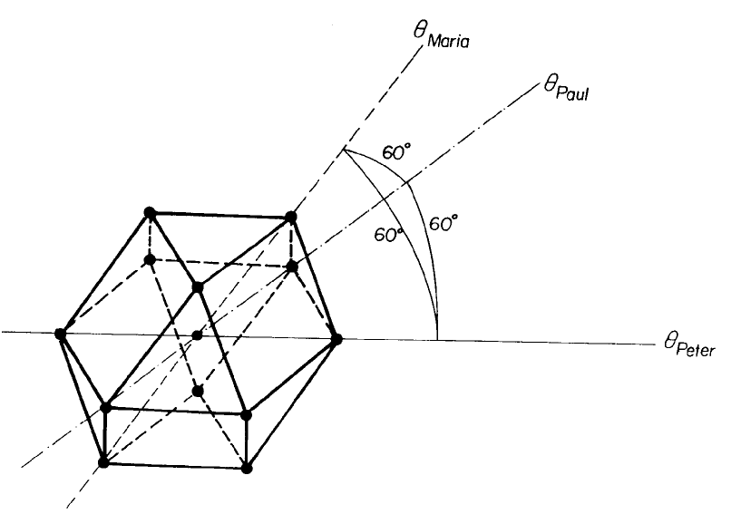
Figure 1: The nearest neighbours of a chosen point in the identification lattice form a cub-octahedron. The metric used is that which corresponds to taking the squared distance as the Manton action.

For the purpose of elucidating the symmetries of the hexagonal identification lattice, it is useful to introduce an extra (superfluous) coordinate $\theta_{4}$. First let us rewrite $S_{\Box\;Manton}$ in (48) as

$$\vec{\theta}^{T}{\bf g}\vec{\theta}=\vec{\theta}^{T}\left\{\frac{\beta}{2}\left(\left(\begin{array}[]{ccc}1/2&0&0\\ 0&1/2&0\\ 0&0&1/2\end{array}\right)+\frac{1}{2}\left(\begin{array}[]{ccc}1&1&1\\ 1&1&1\\ 1&1&1\end{array}\right)\right)\right\}\vec{\theta}=$$ (50)

$$=\frac{\beta}{4}(\theta_{1}^{2}+\theta_{2}^{2}+\theta_{3}^{2}+(\underbrace{-\theta_{1}-\theta_{2}-\theta_{3}}_{\stackrel{{\scriptstyle def}}{{=}}\theta_{4}})^{2})=\frac{\beta}{4}\sum^{4}_{i=1}\theta_{i}^{2}$$

where $\theta_{1}=\theta_{Peter},\cdots,\theta_{3}=\theta_{Maria};\theta_{4}=-\sum_{i=1}^{3}\theta_{i}$.

In this coordinate system with the superfluous coordinate $\theta_{4}$, we have the constraint

$$\sum_{i=1}^{4}\theta_{i}=0$$ (51)

and the hexagonal lattice is characterised as the set of points with coordinates

$$(\theta_{1},\theta_{2},\theta_{3},\theta_{4})\in 2\pi{\bf Z}^{4}.$$ (52)

In this notation, it is apparent that the symmetry group for the lattice and the metric consists of the permutations combined with or without a simultaneous sign shift of all four coordinates.

Each of the 12 nearest neighbours to any site of the identification lattice (e.g. the group identity) have, in the 4-tuple coordinate notation, just two non-vanishing coordinates (that sum to zero). The 1-dimensional subgroups correspond to the 6 co-linear pairs of these 12 nearest neighbours.

The 2-dimensional subgroups are of two types. One type, of which there are 4, are spanned by the identity and any (non-co-linear) pair of the 12 nearest neighbour sites that have a common non-vanishing coordinate. A given subgroup of this type contains 6 nearest neighbour sites positioned at the corners of a hexagon; all 6 such sites of a given 2-dimensional subgroup of this type have a vanishing coordinate in common; e.g., the 6 nearest neighbours with a “0” for the first coordinate belong to the same 2-dimensional subgroup of this type. That there are four such subgroups follows from the fact that there are 4 possibilities for having a common vanishing coordinate in the 4-tuple notation. The other type of 2-dimensional subgroups - there are 3 mutually orthogonal such subgroups - are each spanned by 2 pairs of nearest neighbour sites where the two sites of each such pair have no common non-vanishing coordinates. There are 3 such pairs:

$$\begin{array}[]{c}(\pm 2\pi,0,\mp 2\pi,0)\\ (0,\pm 2\pi,0,\mp 2\pi)\end{array}$$ (53)

$$\begin{array}[]{c}(\pm 2\pi,\mp 2\pi,0,0)\\ (0,0,\pm 2\pi,\mp 2\pi)\end{array}$$ (54)

$$\begin{array}[]{c}(\pm 2\pi,0,0,\mp 2\pi)\\ (0,\pm 2\pi,\mp 2\pi,0).\end{array}$$ (55)

Any of the 3 pairs (53), (54), (55) span one of the $\left(\begin{array}[]{c}3\\ 2\end{array}\right)=3$ orthogonal 2-dimensional subgroups.

The 3-dimensional “subgroup” (which of course is the whole $\mbox{\bf{R}}^{3}$ space) corresponds in the 4-tuple notation to the (whole) hyper-plane specified by

$$\{\vec{\theta}|\sum_{i=1}^{4}\theta_{i}=0\}.$$ (56)

The 0-dimensional subgroup corresponds simply to the identification lattice site that is chosen as the group identity.

4.3.2 Group volume approximation

In this approximation, which is an alternative to the monopole approximation, we calculate the free energy as a function of the couplings for each phase ansatz (i.e. each partially confining phase). The criterion for having a phase in contact with the multiple point is that there is some region of plaquette action parameter space infinitesimally close to the multiple point where the corresponding free energy function is the most stable (i.e., larger than the free energy functions of all the other phases that meet at the multiple point). In previous work[1, 22, 4], we have derived an approximate expression for the free energy per active link. We used the notation $\log Z_{H\triangleleft G}$ for the free energy function corresponding to the phase for which $H$ is the largest confined invariant subgroup of the gauge group $G$:

$$(\log Z_{H\triangleleft G})_{\mbox{\tiny per active link}}=\log\left[\frac{(\pi/6)^{\frac{d_{G}}{2}}}{{\bf\beta}_{G}^{\frac{d_{G}}{2}}vol(G)}\right]+\log\left[\frac{(6\pi)^{\frac{d_{H}}{2}}}{{\bf\beta}_{H}^{\frac{d_{H}}{2}}vol(H)}\right].$$ (57)

where

$${\bf\beta}_{H}^{\frac{1}{2}dim\;H}\stackrel{{\scriptstyle def}}{{=}}\prod_{i}\beta_{i}^{\frac{1}{2}dim\;H_{i}}$$ (58)

and the index $i$ runs over the Lie algebra ideals of $H$.

Consider two partially confining phases in the case that one of these is confined w.r.t to the invariant subgroup $H_{I}$ and the other is confined w.r.t. the invariant subgroup $H_{J}$. At any point in parameter space where these two partially confining phases meet (including the multiple point of course) the condition to be satisfied is $\log Z_{H_{I}\triangleleft G}=\log Z_{H_{J}\triangleleft G}$. This together with (57) leads to the following condition that is fulfilled at any point on the phase boundary separating these two phases:

$$\log(6\pi)^{\frac{dim(H_{J})-dim(H_{I})}{2}}=\log\frac{{\bf\beta}_{H_{J}}^{\frac{dim(H_{J})}{2}}vol(H_{J})}{{\bf\beta}_{H_{I}}^{\frac{dim(H_{I})}{2}}vol(H_{I})}.$$ (59)

We want of course to consider (57) in the special case for which $G=U(1)^{3}$.

Using here a slightly different notation, designate by $\log Z_{H_{n}}$ the free energy per active link for the phase ansatz for which one of the above-mentioned n-dimensional subgroups $H_{n}$ of $U(1)^{3}$ ($dim(H_{n})=n$; $n\in\{0,1,2,3\}$), is confining and the factor group $U(1)^{3}/H_{n}$ behaves in a Coulomb-like way ($H_{n}$ could be one of the 1-dimensional subgroups: e.g., $H_{1}=U(1)_{Peter}$ say). Let us denote by $a$ the lattice constant of the identification lattice. Rewriting (57) and specialising to the case of the gauge group $G=U(1)^{3}$ and $H_{J}=H_{n}$ reveals the dependence of the free energy per active link on the quantity log$a$:

$$\log Z_{H_{n}}=C-(dim(U(1)^{3})+dim(H_{n}))\log a$$ (60)

where $dim(U(1)^{3})=3$ and $dim(H_{n})$ are respectively the dimension of the gauge group (i.e., the $U(1)^{3}$ part of $SMG^{3}$) and the dimension of the subgroup $H_{n}$ and $C$ is a quantity that does not depend on the identification lattice constant $a$. The slope of the various phase ansätze is just

$$\frac{d\log Z_{H_{n}}}{d\log a}=-(dim(U(1)^{3})+dim(H_{n})).$$ (61)

Upon rewriting (59), one obtains for the condition defining the phase boundary between the phase with confinement along the subgroup $H_{n}$ and the phase with confinement along $H_{m}$ the equation

$$(6\pi)^{(dim(H_{n})-dim(H_{m}))/2}=\frac{(\frac{a^{2}}{2\pi^{2}})^{dim(H_{n})/2}c_{n}(2\pi)^{dim(H_{n})}}{(\frac{a^{2}}{2\pi^{2}})^{dim(H_{m})/2}c_{m}(2\pi)^{dim(H_{m})}}\;\;(n,m\in\{0,1,2,3\})$$ (62)

where the volume $vol(H_{n})$ of the subgroup $H_{n}\subseteq U(1)^{3}$, measured in the coordinate $\theta$, is

$$vol(H_{n})=c_{n}(2\pi)^{dim(H_{n})}.$$ (63)

The quantity $c_{n}$ is a factor associated with the subgroup $H_{n}$ that depends on the geometry of the identification lattice.

As an example, consider first a cubic identification lattice (actually we shall end up using an hexagonal lattice as this better satisfies the principle of multiple point criticality). For the cubic lattice with $a=a_{1\;crit}\stackrel{{\scriptstyle def}}{{=}}2\pi\sqrt{\frac{\beta_{crit}}{2}}$, it is possible to have the confluence of three phases of the type corresponding to 1-dimensional subgroups of $U(1)^{3}$ at a multiple point - namely those corresponding to the 1-dimensional subgroups along the $Peter$, $Paul$, and $Maria$ directions of the lattice having $a_{1\;crit}=2\pi\sqrt{\frac{\beta_{crit}}{2}}$ (the subscript “1” on $a_{1\;crit}$ denotes that it is a one dimensional subgroup that is critical). Furthermore, in the case of the cubic identification lattice, it will be seen that phases corresponding to all subgroups of $G=U(1)^{3}$ are simultaneously critical when the identification lattice constant $a=a_{1\;crit}=2\pi\sqrt{\frac{\beta_{crit}}{2}}$. This follows by observing that the free energy $\log Z_{n}$ ($n\in\{0,1,2,3\}$) for the different ansätze (i.e., confinement along the various possible subgroups) are equal for the same value of the identification lattice constant $a$ (i.e., for $a=a_{1\;crit}$) because the constants $c_{n}$ in (62) are independent of the dimension $dim(H_{n})$ of the subgroup (and therefore equal). Hence the condition (62) that defines the boundary between two partially confining phases is independent of dimension. This then means that for the unit cell of the cubic identification lattice, all the quantities $\log Z_{n}$ ($n\in\{0,1,2,3\}$) intersect for $a=a_{1\;crit}=2\pi\sqrt{\frac{\beta_{crit}}{2}}=2\pi\sqrt{\frac{1.01}{2}}=4.465$. So the use of the cubic identification lattice with $a=a_{1\;crit}$ shows that it is possible to have a multiple point at which 8 partially confining phases are in contact: there is one totally confining phase (corresponding to $H_{3}$), three phases corresponding to three 2-dimensional subgroups $H_{2}$, three phases corresponding to three 1-dimensional subgroups $H_{1}$, and a totally Coulomb-like phase corresponding to $H_{0}$. In particular, the coupling corresponding to the diagonal subgroup of $U(1)^{3}$ (in the first approximation, this is the coupling that we identify with the continuum $U(1)$ coupling) is down by a factor $\sqrt{3}$ relative to the critical coupling for a $U(1)$ lattice gauge theory. This follows because the inverse of the ratio of the length of the diagonal to the critical lattice constant is $\sqrt{3}$. Phenomenologically, a factor of roughly $\sqrt{6}$ rather than $\sqrt{3}$ is needed so we must conclude that for the $U(1)$ continuum coupling, the prediction of the multiple point criticality principle using a cubic identification lattice is at odds with experiment.

However, the multiple point criticality principle states that we should seek the values of the continuum $U(1)$ coupling at a point in parameter space at which a maximum number of phases come together. We have already seen that for a hexagonal identification lattice in the covering group $\mbox{\bf{R}}^{3}$ of the gauge group $U(1)^{3}$, we can, in terms of the 12 nearest neighbours of a site in the hexagonal identification lattice, identify a total of 15 subgroups corresponding to 15 partially confining phases. Even though we shall discover in the sequel that 3 of these 15 partially confining phases - the 2-dimensional “orthogonal” phases given by (53-55) - are not realistically realizable in the volume approximation inasmuch as these phases are “pushed” too far away from the multiple point in the volume approximation, there remains 12 partially confining phases that can be made to convene at the multiple point. This is, in view of the multiple point criticality principle, an improvement upon the total of 8 phases that can be realized at the multiple point in the case of the cubic identification lattice.

It will be seen that the price we must pay for realizing these 12 remaining partially confining phases at the multiple point in the case of the hexagonal identification lattice instead of the 8 partially confining phases of the cubic identification lattice is that these 12 phases no longer come together exactly at a common value of the identification lattice constant $a$ if we use a pure Manton action (36).

For the hexagonal identification lattice, the problem is that when the lattice constant $a$ is chosen so that $a=a_{1\;crit}\stackrel{{\scriptstyle def}}{{=}}2\pi\sqrt{\frac{\beta_{crit}}{2}}$ corresponding to criticality for the 1-dimensional subgroups, this choice fixes the values of the couplings for the 2- and 3-dimensional subgroups at sub-critical values. For example, for $a=a_{1\;crit}$, the free energy functions $\log Z_{0}$ and $\log Z_{1}$ are equal corresponding to the coexistence of the totally Coulomb-like phase and the six phases that are confined along 1-dimensional subgroups. However, if for example one wishes to have coexistence of the totally Coulomb-like phase and the four phases that are confined along the four 2-dimensional subgroups, it will be seen (Table 2) that $\log a$ must be decreased by $\frac{1}{4}\log(4/3)$. But this reduction in $\log a$ would put the phases corresponding to 1-dimensional subgroups into confinement.

Information about the cubic and hexagonal lattices are tabulated in Tables 1 and 2. Table  1 pertains to the cubic lattice; Table  2 to the hexagonal identification lattice. The entries in the first four (five) rows and columns of Table 1 (Table 2) give the values of the identification lattice constant $a^{2}$ (in terms of $a^{2}_{1\;crit}$) at which pairs (corresponding to a row and column heading) of free energy phase ansätze intersect; i.e., these entries are the quantities

$$\frac{a^{2}}{a^{2}_{1\;crit}}=\left(\frac{c_{n}}{c_{m}}\right)^{\frac{-2}{dim(H_{n})-dim(H_{m})}}\;\;\;\;(n,m\in\{0,1,2,3\})$$ (64)

obtained by rewriting (62) and using that $a_{1\;crit}^{2}=3\pi$ (obtained from (62) with $n=1$ and $m=0$. The quantities $a$ and $a_{1,\;crit}=2\pi\sqrt{\frac{\beta_{crit}}{2}}$ are respectively the identification lattice constant and the critical value of the (identification) lattice constant. The quantities $c_{n}$ are the volume correction factors associated with the subgroup $H_{n}$ ($n\in\{0,1,2,3\}$). These are also tabulated in the tables below. All the volume correction factors are unity for the cubic identification lattice. For the hexagonal lattice, $c_{0}$ and $c_{1}$ are both unity whereas $c_{2}=\sqrt{3/4}$ and $c_{3}=\sqrt{1/2}$ corresponding respectively to the ratio of area of a minimal parallelogram in the hexagonal lattice to the area of a simple plaquette in the cubic lattice and the ratio of the volume of a (minimal) parallelpipidum of the hexagonal lattice to the volume of a simple cube in the cubic lattice.

Table 1: Parameters pertaining to the cubic identification lattice. The entries in the first four rows and columns are all unity because phases corresponding to all subgroups convene at the multiple point for the critical value of the coefficient $\frac{1}{e^{2}_{U(1)\;crit}}$ in the Manton action; i.e., the quantity $\frac{a^{2}}{a^{2}_{1\;crit}}=\left(\frac{c_{n}}{c_{m}}\right)^{\frac{-2}{dim(H_{n})-dim(H_{m})}}$ $(n,m\in\{0,1,2,3\})$ is unity for all $m,n\in\{0,1,2,3\}$. The quantities in the last three columns are as explained in Table (2).

CUBIC	$\log Z_{H_{0}}$	$\log Z_{H_{1}}$	$\log Z_{H_{2}}$	$\log Z_{H_{3}}$	$\frac{d\log Z_{H_{n}}}{d\log a}$	# phases	$c_{n}$
$\log Z_{H_{0}}$	1	1	1	1	-3	1	1
$\log Z_{H_{1}}$		1	1	1	-4	3	1
$\log Z_{H_{2}}$			1	1	-5	3	1
$\log Z_{H_{3}}$				1	-6	1	1

Table 2: Parameters pertaining to the hexagonal identification lattice. As regards the five rows and first five columns, the entry in the n$th$ column and the m$th$ row is the coefficient $\frac{a^{2}}{a^{2}_{1\;crit}}=\left(\frac{c_{n}}{c_{m}}\right)^{\frac{-2}{dim(H_{n})-dim(H_{m})}}$ $(n,m\in\{0,1,2,3\})$ . This is the quantity by which $\frac{1}{e^{2}_{U(1)\;crit}}$ must be multiplied in order that the phases confined w.r.t. the $n$-dimensional and $m$-dimensional subgroups can come together at the multiple point. The slope of the $\frac{d\log Z_{H_{m}}}{d\log a}$, calculated from (61), is given in the sixth column. Column seven gives the number of phases of dimension $m$. The entries in column eight are the “volume” correction factors $c_{n}$ (see (63)) in the hexagonal lattice relative to the corresponding (unit) “volumes” in the cubic lattice.

HEXAG.	$\log Z_{H_{0}}$	$\log Z_{H_{1}}$	$\log Z_{H_{2}orthog}$	$\log Z_{H_{2}}$	$\log Z_{H_{3}}$	$\frac{d\log Z_{H_{n}}}{d\log a}$	# phases	$c_{n}$
$\log Z_{H_{0}}$	1	1	1	$\sqrt{\frac{4}{3}}$	$\sqrt[3]{2}$	-3	1	1
$\log Z_{H_{1}}$		1	1	$\frac{4}{3}$	$\sqrt{2}$	-4	6	1
$\log Z_{H_{2}orthog}$			1		2	-5	3	1
$\log Z_{H_{2}}$				1	$\frac{3}{2}$	-5	4	$\sqrt{\frac{3}{4}}$
$\log Z_{H_{3}}$					1	-6	1	$\sqrt{\frac{1}{2}}$

However, the amount by which the free energy functions for these different phases fail to intersect at a common value of the identification lattice is hopefully small enough to be dealt with meaningfully by perturbing the Manton action (using 4$th$ and 6$th$ order terms) in such a way as to allow 12 phases to convene at a multiple point.

We therefore replace the Manton action (containing by definition only second order terms) by a more complicated action:

$$S_{\Box,\;Manton}\rightarrow S_{\Box,\;Manton}+S_{\Box,\;h.o.}$$

where $S_{\Box,\;h.o.}$ designates higher than second order terms. In choosing the higher order terms, we want to use the lowest possible order terms that bring together the desired phases at the multiple point.

The number of additional terms needed depends on how many phases we want to bring together at the multiple point. As explained above, we have decided to settle for the 12 phases (corresponding to one 0-dimensional, six 1-dimensional, four 2-dimensional, and one 3-dimensional subgroups) that have the smallest possible volume on the hexagonal lattice and which are not too far from being able to convene at the multiple point with the Manton action alone. These 12 phases seem to exhaust the ones for which a modification of the couplings using the procedure to be explained below can be regarded as a small perturbation; for example, the diagonal subgroup coupling (with pure Manton action) is so far removed from the critical couplings of the 12 hexagonal lattice phase discussed above that we a priori give up trying to have a phase confined along the diagonal subgroup in contact with the multiple point. The same applies presumably to the 2-dimensional “orthogonal” subgroups (53-55) as already mentioned above.

Due to the high degree of symmetry of the hexagonal lattice, the conditions for the criticality are identical for phases corresponding to the four 2-dimensional subgroups and the six 1-dimensional subgroups. So the number of parameters we need to get all 12 phases to convene is effectively that for four phases (corresponding to the four possible dimensionalities of subgroups). This requires 4-1=3 parameters. This can be compared to the generic number of parameters necessary for the meeting of 12 phases: 12-1=11 parameters. The point is that the symmetry of the hexagonal identification lattice allows a non-generic multiple point in an action parameter space spanned by just three parameters. These can be chosen as the Manton parameter (i.e., the coefficient to the second order term in a Taylor expansion of the action) and two parameters that are coefficients to respectively a 4th and a 6th order term. These 4th and 6th order terms are to be chosen so as to have the same symmetry as the hexagonal lattice; otherwise we lose the symmetry that allows a non-generic multiple point. Without the symmetry, we would in general need 11 parameters instead of 3. It is also necessary that these two terms contribute differently to the different free energy functions for the different types of subgroup that we want to bring to the multiple point. Otherwise we could compensate for the effect of these higher order terms for all subgroups by using a single new effective coefficient to the Manton term. In other words, we want our high order terms to be such that these give different new effective coefficients to the second order action term for different subgroups. The effective second order coefficient is defined as the coefficient in the Manton action that would give the same fluctuation width inside the subgroup in question as there would be with the higher order terms in place. To this end we use linear combinations of spherical harmonics $Y_{lm}$ with $l=4$ and $l=6$ that have the same symmetry as the cub-octahedron (which can be taken as the “unit cell” of the hexagonal identification lattice). These linear combinations, denoted $Y_{4\;comb}$ and $Y_{6\;comb}$, are invariant under the symmetry of the cub-octahedron.

In using the $Y_{4\;comb}$ and $Y_{6\;comb}$ as perturbations to the Manton action, we obtain an effective Manton inverse squared coupling strength that varies with the direction $\vec{\xi}$:

$$\frac{1}{e^{2}_{eff}(\vec{\xi})}.$$ (65)

Here $\vec{\xi}$ denotes a vector in $\mbox{\bf{R}}^{3}$ (the covering space of $U(1)^{3}$).

The desired combinations $Y_{4\;comb}$ and $Y_{6\;comb}$ that have the symmetry of the cub-octahedron turn out, after a rather strenuous calculation, to be

$$Y_{4\;comb}=\frac{2}{3}\sqrt{7}Y_{40}+\frac{4}{3}\sqrt{5}(Y_{43}+Y_{4,-3})/i\sqrt{2}$$ (66)

and

$$Y_{6\;comb}=(-4\sqrt{\frac{3}{35}})Y_{60}+\sqrt{\frac{11}{10}}(Y_{66}+Y_{6,-6})/\sqrt{2}+(Y_{63}+Y_{6,-3})/i\sqrt{2}.$$ (67)

These have been calculated in a coordinate system in which the $z$-axis coincides with a 3-axis of symmetry of the cub-octahedron. In Table 3 these combinations $Y_{4\;comb}$ and $Y_{6\;comb}$ are averaged over the 1,2 and 3-dimensional subgroups of $U(1)^{3}$. The fact that both combinations vanish for $U(1)^{3}$ (the 3-dimensional subgroup) reflects of course the property that spherical harmonics vanish when integrated over the surface of a sphere. Table 3 also gives the values of $Y_{4\;comb}$ and $Y_{6\;comb}$ along the diagonal subgroup of $U(1)^{3}$.

Table 3: The $4th$ and $6th$ order action contributions needed to realize 12 partially confining phases at the multiple point. The contributions have the symmetry of the hexagonal identification lattice.

$$\begin{array}[]{|c|c|c|}\hline\cr\mbox{subgroup}&Y_{4\;\;comb}&Y_{6\;\;comb}\\ \hline\cr\langle Y_{l\in\{4,6\}}\rangle_{3-dim}&0&0\\ \hline\cr\langle Y_{l\in\{4,6\}}\rangle_{2-dim}&\frac{\sqrt{7}}{4}&\frac{5}{4}\sqrt{\frac{3}{35}}\\ \hline\cr Y_{l\in\{4,6\};\;1-dim}&\frac{\sqrt{7}}{4}&\frac{117}{32}\sqrt{\frac{3}{35}}\\ \hline\cr Y_{l\in\{4,6\};\;diagsubgr}&\frac{2\sqrt{7}}{3}&-4\sqrt{\frac{3}{35}}\\ \hline\cr\end{array}$$ (68)

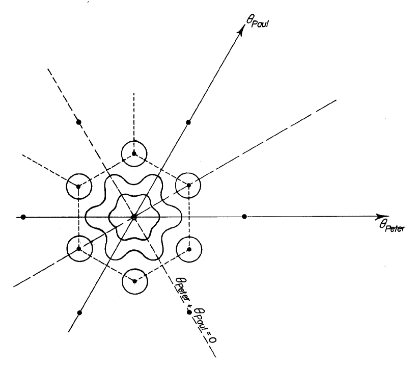
Figure 2: Contours of constant perturbed Manton action for $U(1)^{2}$ represented in the covering group $\mbox{\bf{R}}^{2}$ with the metric in the plane of the paper that is identified with the Manton action metric. The hexagonal lattice of “$\bullet$” are points identified in compactifying from $\mbox{\bf{R}}^{2}$ to $U(1)^{2}$. The purpose of the correction - it is sixth order and gives the contours a “webbed feet” look - is to increase $\log Z$ for the phases with confinement along one of the three 1-dimensional subgroups - i.e., along the $\theta_{Peter}$ axis, the $\theta_{Paul}$ axis and along the line given by $\theta_{Peter}+\theta_{Paul}=0$ - while disfavouring fluctuations along directions that bisect the angles between these 1-dimensional subgroup directions. This is accomplished by decreasing the gradient of the action in these three subgroup directions while increasing the gradient in directions that bisect the above-mentioned three subgroups

Using the Tables 1, 2, and 3, let us now determine the coefficients to the 2$nd$ order (i.e. Manton) as well as 4$th$ and 6$th$ order action terms by using the requirement that averages over the 1, 2 and 3-dimensional subgroups of $U(1)^{3}$ are equal to the $U(1)$ critical inverse squared coupling $1/e^{2}_{U(1)\;crit}$ when the volume correction factors for the hexagonal lattice are taken into consideration. These latter are given by (64). Using that $\beta=1/e^{2}=a^{2}/2\pi^{2}$ we can write the condition to be satisfied if the average over the subgroup $H_{n}$ - i.e., $\langle 1/e^{2}(\vec{\xi})\rangle_{H_{n}}$ - is to have a value corresponding to the boundary between a phase confined along $H_{n}$ and the totally Coulomb phase:

$$\langle\frac{1}{e^{2}(\vec{\xi})}\rangle_{H_{n}}=\left(\frac{c_{n}}{c_{0}}\right)^{\frac{-2}{dim(H_{n})-dim(H_{0})}}\frac{1}{e^{2}_{U(1)\;crit}}$$ (69)

where $c_{0}$ and $H_{0}$ correspond to the totally Coulomb phase. Eqn. (69) yields three equations - one for each type of subgroup $H_{n}$ ($n=dim(H_{n})$).

For $n=3$ there are no contributions to $\langle\frac{1}{e^{2}_{eff}(\vec{\xi})}\rangle_{3-dim\;subgr}$ from $Y_{4\;comb}$ and $Y_{6\;comb}$. The second order coefficient $\frac{1}{e_{Manton}^{2}}$ is therefore determined by the one equation

$$\langle\frac{1}{e^{2}_{eff}(\vec{\xi})}\rangle_{3-dim\;subgr}=\frac{1}{e_{Manton}^{2}}=\left(\frac{c_{3}}{c_{0}}\right)^{\frac{-2}{3-0}}\frac{1}{e^{2}_{U(1)\;crit}}=2^{\frac{1}{3}}\frac{1}{e^{2}_{U(1)\;crit}}.$$ (70)

The coefficients to $Y_{4\;comb}$ and $Y_{6\;comb}$ - denoted respectively as $B_{4}$ and $B_{6}$ - can be obtained from the equations for $\langle\frac{1}{e^{2}_{eff}(\vec{\xi})}\rangle_{1-dim\;subgr}$ and $\langle\frac{1}{e^{2}_{eff}(\vec{\xi})}\rangle_{2-dim\;subgr}$. Assigning dimensionality to the strictly speaking dimensionless quantity $1/e^{2}$, we use that [$B_{4}$]=[$\frac{1}{e^{4}}$] and [$B_{6}$]=[$\frac{1}{e^{6}}$].

For $n=1$ we have:

$$\langle\frac{1}{e^{2}_{eff}(\vec{\xi})}\rangle_{1-dim\;subgr}^{3}=B_{6}\langle Y_{6\;comb}\rangle_{1-dim\;subgr}+\left(\frac{1}{e^{4}_{Manton}}+B_{4}\langle Y_{4\;comb}\rangle_{1-dim\;subgr}\right)^{\frac{3}{2}}=$$ (71)

$$=B_{6}\frac{117}{32}\sqrt{\frac{3}{35}}+\left(\frac{2^{\frac{2}{3}}}{e^{4}_{U(1)\;crit}}+B_{4}\frac{\sqrt{7}}{4}\right)^{\frac{3}{2}}=\left(\left(\frac{c_{1}}{c_{0}}\right)^{\frac{-2}{3-0}}\frac{1}{e^{2}_{U(1)\;crit}}\right)^{3}=\left(1\frac{1}{e^{2}_{U(1)\;crit}}\right)^{3}.$$

For $n=2$ we have:

$$\langle\frac{1}{e^{2}_{eff}(\vec{\xi})}\rangle_{2-dim\;subgr}^{3}=B_{6}\langle Y_{6\;comb}\rangle_{2-dim\;subgr}+\left(\frac{1}{e^{4}_{Manton}}+B_{4}\langle Y_{4\;comb}\rangle_{2-dim\;subgr}\right)^{\frac{3}{2}}=$$ (72)

$$=B_{6}\frac{5}{4}\sqrt{\frac{3}{35}}+\left(\frac{2^{\frac{2}{3}}}{e^{4}_{U(1)\;crit}}+B_{4}\frac{\sqrt{7}}{4}\right)^{\frac{3}{2}}=\left(\left(\frac{c_{2}}{c_{0}}\right)^{\frac{-2}{2-0}}\frac{1}{e^{2}_{U(1)\;crit}}\right)^{3}=\left(\sqrt{\frac{4}{3}}\frac{1}{e^{2}_{U(1)\;crit}}\right)^{3}.$$

The values of the geometric factors $c_{n}$ are from Table 2 and the values of $\langle Y_{6\;comb}\rangle_{n-dim\;subgr\;H_{n}}$ and $\langle Y_{4\;comb}\rangle_{n-dim\;subgr\;H_{n}}$ $(n=dim(H_{n})\in\{0,1,2,3\})$ are taken from Table 3.

Solving these equations for the coefficients $B_{4}$ and $B_{6}$ yields

$$B_{4}=-0.1463\mbox{ and }B_{6}=-0.7660$$ (73)

We have now succeeded in fitting three coefficients of a modified Manton (i.e. a plaquette action dominated by a second order “Manton” term but having perturbative 4$th$ and 6$th$ order terms) in such a way that 4 types of phases $H_{n}$ convene at a multiple point in the sense that $\langle 1/e^{2}_{eff}(\vec{\xi})\rangle_{H_{n}}$ ($n=dim(H_{n})\in\{0,1,2,3\}$) is equal to the $U(1)$ critical coupling up to a factor pertaining to the geometry of the hexagonal identification lattice. Because the modified Manton action has the symmetry of the hexagonal lattice, multiple point criticality for a phase corresponding to a given dimension implies multiple point criticality for all phases corresponding to a given dimension. For this reason we achieve multiple point criticality for a total of 12 phases. The averaging $\langle 1/e^{2}_{eff}(\vec{\xi})\rangle_{H_{n}}$ can be taken as an average over all directions within the subgroup $H_{n}$ using a measure defined by being invariant under rotations leaving the Manton metric invariant.

So we now have at our disposal a means of calculating a directionally dependent effective inverse squared coupling where the directional dependence comes from the perturbative $4th$ and $6th$ order action terms. In a later section, we shall want to calculate $1/e^{2}_{eff}$ in the direction corresponding to the diagonal subgroup (in a chosen coordinate system).

5 Calculation of the numerical value of the continuum coupling

5.1 Outline of procedure

The aim now is to calculate the continuum $U(1)$ standard model weak hyper-charge coupling corresponding to the “diagonal subgroup” coupling at the multiple point of the $AGUT$ gauge group $SMG^{3}$. In principle, the multiple point should be sought in a very high dimensional action parameter space that is also in contact with a multitude of phases that are alone confined w.r.t discrete $\mbox{\bf{Z}}_{N}$ subgroups. In an even more correct search for the multiple point involving phases with confining discrete subgroups, we should really consider Abelian and non-Abelian groups at the same time (i.e, the full $SMG^{3}$ or perhaps an even larger group) because discrete subgroups having the characteristic of being non-factorizable could a priori simultaneously involve Abelian subgroups and centres of semi-simple subgroups.

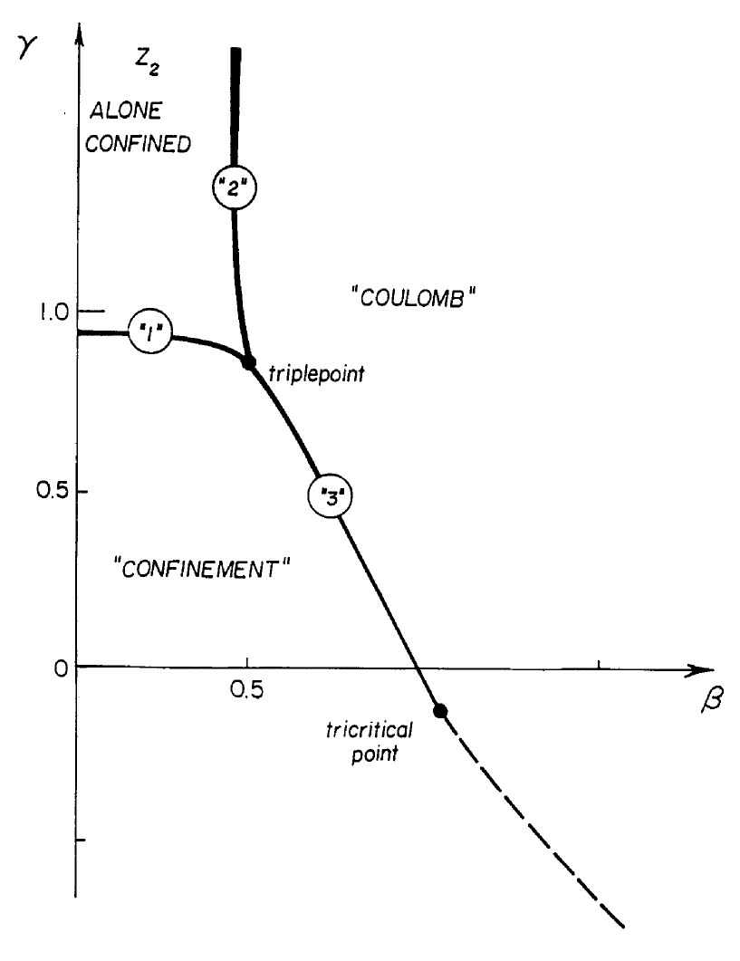
Figure 3: The phase diagram for $U(1)$ when the two-parameter action is used. This type of action makes it possible to provoke the confinement of $\mbox{\bf{Z}}_{2}$ (or $\mbox{\bf{Z}}_{3}$) alone.

As a crude prototype to a $U(1)^{3}$ phase diagram, we consider the (generic) phase diagram spanned by the parameters of an action with $\cos\theta,\cos\frac{\theta}{2}$ and $\cos\frac{\theta}{3}$ terms. This action, which is one of the simplest generalisations of the pure Wilson action, has been studied extensively[15] and many features of the phase diagram (Figure 3) are well understood. From the triple point (TP) (which is the “multiple point” in this 2-dimensional phase diagram) emanate three characteristic phase borders: the phase border “3” separates the totally confining and totally Coulomb-like phases; the phase border “1” separates the totally confining phase from the phase where only the discrete subgroup $\mbox{\bf{Z}}_{2}$ is confined; this latter phase is separated from the totally Coulomb-like phase by the phase border “2”.

The calculational procedure to be used in determining the continuum $U(1)$ coupling is approximative and is done in two steps:

1. first we calculate the factor analogous to the factor $3=N_{gen}$ in the non-Abelian case; we call this the enhancement factor and denote it as $\frac{1/\alpha_{U(1)^{3}\;diag}}{1/\alpha_{U(1)_{crit\;TP}}}$. This factor lies in the range 6.0 - 8.0 depending on the degree of “first-orderness” of the triple point (TP) transition at boundary “2”.

2. In the second step, the continuum $U(1)$ coupling corresponding to the multiple point value for a single $U(1)$ is determined using an analogy to a procedure proposed by Luck[27] and developed by Jersàk[18].

This two-step calculation can be done using more or less good approximations as regards the extent to which the continuum $U(1)$ coupling value reflects having phases solely confining w.r.t. discrete subgroups among the phases that convene at the multiple point. Let us outline the possible approximations in the order of increasing goodness.

1. The roughest calculation would be to use a single parameter action with hexagonal symmetry without regard to having phases at the triple point (TP) that are confining solely w.r.t. the discrete subgroups $\mbox{\bf{Z}}_{2}$ and $\mbox{\bf{Z}}_{3}$ of $U(1)^{3}$. In this approximation, these discrete subgroups are treated as though they were totally confining inasmuch as it is a $U(1)$-isomorphic factor group obtained essentially by dividing $\mbox{\bf{Z}}_{2}\times\mbox{\bf{Z}}_{3}$ out of the $U(1)$ centre of $SMG$ that is identified with the lattice $U(1)$ critical coupling.

2. By using a two-parameter action (later a three parameter action) leading to the phase diagram of Figure 3, the action now acquires a (nontrivial) dependence on the elements within the cosets of the factor group $U(1)/\mbox{\bf{Z}}_{2}$ (or the factor group $U(1)/(\mbox{\bf{Z}}_{2}\times\mbox{\bf{Z}}_{3})$ in the case of a three-parameter action) that can reveal how close the discrete subgroups are to being critical. However these details are of little importance to the $U(1)$ continuum coupling; the latter depends essentially only on a single yet to be defined parameter $\gamma_{eff}$ the critical value of which is very nearly constant along the phase boundary “1” of Figure 3. Hence the $U(1)$ continuum coupling is also approximately constant along this phase boundary in accord with the rule described in the footnote on page 17. The critical value $\gamma_{eff\;crit}$ of the parameter $\gamma_{eff}$ is expressible in terms of the critical lattice parameters available from computer data for a lattice gauge theory with a single $U(1)$.

3. The effect on the continuum coupling of having phases convening at the multiple point that are confined solely w.r.t. $\mbox{\bf{Z}}_{2}$ and solely w.r.t. $\mbox{\bf{Z}}_{3}$ appears first when we take into account the discontinuity in $\Delta\gamma_{eff}$ encountered in crossing the boundary “2” at the multiple point. As we in both steps A. and B. above want to use the value of $\gamma_{eff}$ corresponding to the totally Coulomb-like phase at the multiple point, it is important for our calculation of the $U(1)$ continuum coupling to take the “jump” $\Delta\gamma_{eff}$ into account. Inasmuch as the continuum subgroup degrees of freedom are in the same phase on both sides of boundary “2”, this discontinuity $\Delta\gamma_{eff}$ is entirely due to a phase transition for the discrete subgroup(s). Moreover, the presence of a discontinuity presumably reflects the degree of first-orderness of the triple point transition at border “2” inherited from a pure $\mbox{\bf{Z}}_{2}$ and $\mbox{\bf{Z}}_{3}$ transition (i.e., for $\gamma>>1$ in Figure 3).

4. The discrete subgroups $\mbox{\bf{Z}}_{2}$ and $\mbox{\bf{Z}}_{3}$ contribute differently to the “jump” $\Delta\gamma_{eff}$ in crossing the boundary “2” due to the fact that $\mbox{\bf{Z}}_{2}^{3}$ does not inherit the hexagonal symmetry of $U(1)^{3}$ while $\mbox{\bf{Z}}_{3}^{3}$ is more likely to do so. This is discussed at the end of Section 4.2.

It is important to recall that the normalisation of the $U(1)$ that we have argued for is implemented by the identification of the $U(1)$ lattice critical coupling with the ($U(1)$-isomorphic) factor-group $=SMG/(SU(2)\times SU(3))$ for some one of the Cartesian product factors say $SMG_{Peter}$. Since we have argued or assumed that phases with genuine discrete subgroups of this $U(1)$ factor-group are not to be in contact with the multiple point chosen by Nature, the only discrete subgroups that are to be taken into account are discrete subgroups of the $U(1)$ subgroup of $SMG$. The relation between the $U(1)$ subgroup and the factor-group $SMG/(SU(2)\times SU(3))$ can be described as $U(1)_{factorgr}=U(1)_{subgr}/{\bf Z}_{6}$.

In using $U(1)/\mbox{\bf{Z}}_{6}$ as the factor group to be identified with the lattice critical $U(1)$, we identify the elements of $\mbox{\bf{Z}}_{6}$ and thereby “hide” any differences that there might be in the probabilities for being at different elements of $\mbox{\bf{Z}}_{6}$ when a one-parameter action is used (approximation 1 in list above). But the details of how the heights of the peaks in probability at different elements of $\mbox{\bf{Z}}_{6}$ differ are important if we want to arrange that the discrete subgroups of $\mbox{\bf{Z}}_{6}$ are by themselves to be confined in phases convening at the triple point. However such details become visible again if the (one-parameter) Wilson action (roughest approximation 1 in the list above) is replaced by the (two-parameter) “mixed” fundamental-adjoint action (approximation 2 and 3 in the list above). By introducing an additional parameter in this way, we render the group elements identified in the factor groups $U(1)_{subgr}/\mbox{\bf{Z}}_{2}$ and $U(1)_{subgr}/\mbox{\bf{Z}}_{3}$ inequivalent (i.e., the action acquires a dependence on the elements within the cosets of these factor groups). So in effect, by going from the Wilson action to the two-parameter action we lift the factor group up into a kind of covering space. The result is that by replacing the $U(1)_{factorgr}$ critical coupling by the triple point coupling for the $U(1)_{subgr}$ of $SMG$, we essentially arrange that the subgroups ${\bf Z}_{2}$ and ${\bf Z}_{3}$ can confine individually in phases that convene at the triple point (TP).

In both steps A. and B. of the calculation of the continuum $U(1)$ coupling, we make use of the “jump” $\Delta\gamma_{eff}$ in the quantity $\gamma_{eff}$ that in Section 5.2 below will be argued to be an effective coupling in the sense that in the region of the phase diagram near the phase border “1” in Figure 3 (i.e., on both sides of “1”) it is to a good approximation valid that the phase realized (i.e., the totally confined or the phase with only $\mbox{\bf{Z}}_{2}$ confined) is determined by the value of this one variable $\gamma_{eff}$ ($\gamma_{eff}$ is a certain combination of the parameters $\gamma$ and $\beta$ of the two-parameter action (see Figure 3)). Consequently, the variable $\gamma_{eff}$ is necessarily constant along the phase boundary “1” and we can also assume that the corresponding continuum coupling has a constant value along this boundary. The change in $\gamma_{eff}$ - i.e. $\Delta\gamma_{eff}$ - comes first at the boundary “2” in going into the totally Coulomb-like phase. The value of $\Delta\gamma_{eff}$ (calculated in Section 5.3) depends on the degree of “first-orderness” that at the multiple point ($\gamma\approx 1$) is inherited from the pure $\mbox{\bf{Z}}_{2}$ and $\mbox{\bf{Z}}_{3}$ transitions at $\gamma\rightarrow\infty$. Without the correction for discrete subgroups embodied by $\Delta\gamma_{eff}$, the multiple point coupling is obtained as if the discrete subgroups were totally confining.

In the step A., the quantity $\Delta\gamma_{eff}$, which reflects the degree of first-orderness inherited from the pure $\mbox{\bf{Z}}_{2}$ and $\mbox{\bf{Z}}_{3}$ transition in crossing boundary “2” at the multiple point, is used to interpolate between the enhancement factor of about 8 obtained with the volume approximation and the enhancement factor of 6 obtained with the independent monopole approximation. These approximations are most suitable for respectively first and second order transformations. The calculation of the enhancement factor is done in Section 5.4.

In step B. of the calculation (performed in Section 5.5), the quantity $\Delta\gamma_{eff}$ is again used - this time in the combination $\gamma_{eff}+\Delta\gamma_{eff}$ - to calculate the $U(1)$ continuum coupling corresponding to the triple point values of a (single) $U(1)$ lattice gauge theory. We seek the continuum coupling in the corner of the totally Coulomb-like phase (necessary if Planck-scale confinement of observed fermions is to be avoided) that lies at the triple point - that is, in the “corner” formed by the phase borders “2” and “3”. According to the above argumentation, we know that the continuum coupling at any position along the border “1”: it is just equal to the value at $\gamma=\gamma_{crit}$ and $\beta=0$. In particular, this is true at the multiple point in the phase with only $\mbox{\bf{Z}}_{2}$ confining (i.e., in the “corner” formed by the phase boundaries “1” and “2”). But as argued above, we want the coupling corresponding to the Coulomb phase “corner” formed by borders “2” and “3”. This requires a correction that accounts for going from the multiple point corner formed by “1” and “2” to the multiple point corner formed by borders “2” and “3” (and in principle also a small correction from crossing border “1”). It is this transition, corresponding to the transition from a phase with solely $\mbox{\bf{Z}}_{2}$ confining to a totally Coulomb-like phase that is accompanied by the “jump” denoted by $\Delta\gamma_{eff}$.

5.2 The approximation of an effective $\gamma$

In the literature ([15, 16]) we find the phase diagram for a $U(1)$ group with a mixed lattice action having a $\gamma$ term defined on the factor-group $U(1)/{\bf Z}_{2}$:

$$S_{\Box}(\theta)=\gamma cos(2\theta)+\beta cos(\theta).$$ (74)

With this action it is easy to provoke confinement of the whole group as well as the totally Coulomb phase and phase confined solely w.r.t. a discrete subgroup isomorphic to $\mbox{\bf{Z}}_{2}$ for a judicious choice of the action parameters $\gamma$ and $\beta$ that span the phase diagram in Figure 3. Indeed the phase diagram of Figure 3 clearly reveals a triple point common to three phases. The interpretation of these phases as the three referred to above is confirmed by rough mean field estimates for the phase borders. In the case of the non-Abelian subgroups $SU(2)$ and $SU(3)$, two of the phases in Figure 3 are actually connected, because one of the phase borders ends at a tri-critical point. However, this does not of course preclude the existence of a multiple (i.e., triple) point.

Before proceeding, it is useful to change notation by scaling the variable $\theta$ down by a factor two inasmuch as it is recalled (see 3.1.1) that we want to normalise relative to the factor group $U(1)/\mbox{\bf{Z}}_{2}$.

$$S_{\Box}(\theta)=\gamma\cos(\theta)+\beta\cos(\theta/2).$$ (75)

Note that with this notational convention, Bianchi identities are fulfilled modulo $4\pi$. In discussions of monopoles dealt with in later sections, we shall have occasion to distinguish “full” $4\pi$-monopoles and “minimal strength” $\frac{2\pi}{4\pi}$-monopoles. The latter will be seen to correspond to the “length” of the factor group $U(1)/\mbox{\bf{Z}}_{2}$. These remarks first become relevant and more transparent when, in a later section, we explain the idea of “minimal strength” monopoles. In the case of $\mbox{\bf{Z}}_{2}$, such monopoles are referred to as $\frac{2\pi}{4\pi}$-monopoles. These will be seen to be the monopoles present relative to a $\mbox{\bf{Z}}_{2}$ background field.

In order to obtain numerical results, the multiple point coupling in this diagram will in a later Section be related to the point at which $\beta=0,\gamma=\gamma_{critical}$ inasmuch as we have a procedure for relating this point to the continuum coupling at the triple point (hereafter “TP”) “corner” formed by the phase boundaries “1” and “2” and subsequently at the for us interesting TP “corner” formed by the phase boundaries “2” and “3” (i.e., the totally Coulomb phase at the TP - see Figure 3). We shall actually argue that to a very good approximation the continuum coupling does not vary along the phase border “1” (separating the “total confinement” and the “phase with only ${\bf Z}_{2}$ confining”) in going from $(\beta,\gamma)=(0,\gamma_{crit})$ to the corner at the TP formed by the phase boundaries “1” and “2”. It is first upon crossing the phase boundary “2” into the totally Coulomb phase at the TP that there is a change - a jump $\Delta\gamma_{eff}$ - in the quantity $\gamma_{eff}$ that immediately below will be seen to be an effective coupling. This jump $\Delta\gamma_{eff}$ comes from a jump in the relative probability of finding the plaquette variable at the(a) non-trivial element of $Z_{2}(\mbox{\bf{Z}}_{3})$ upon making the transition at boundary “2” separating the totally Coulomb-like phase from the phase solely confined w.r.t. $\mbox{\bf{Z}}_{2}$ or $\mbox{\bf{Z}}_{3}$ in Figure 3. As the continuum degrees of freedom are in the same phase on both sides of the boundary “2”, the discontinuity $\Delta\gamma_{eff}$ must be entirely due to the discrete subgroup transition which inherits a considerable degree of the first order nature of the pure (i.e., for $\gamma\rightarrow\infty$) discrete group transition.

In order to see how the effective coupling $\gamma_{eff}$ comes about, we consider the partition function for the action (75)

$$Z=\int{\cal D}\theta(\mbox{\begin{picture}(4.15,10.0)\put(0.0,3.0){\circle*{2.0}} \put(0.0,2.75){\line(1,0){7.0}} \put(7.3,3.0){\circle*{2.0}}\mbox{ } \end{picture} })\exp(\sum_{\Box}(\gamma cos(\theta)+\beta cos(\theta/2))).$$ (76)

It can be rewritten as

$$Z=\int{\cal D}\hat{\theta}(\mbox{\begin{picture}(4.15,10.0)\put(0.0,3.0){\circle*{2.0}} \put(0.0,2.75){\line(1,0){7.0}} \put(7.3,3.0){\circle*{2.0}}\mbox{ } \end{picture} })\exp(\sum_{\Box}(\gamma\cos(\hat{\theta})+\log(\cosh(\beta(\cos(\hat{\theta}/2)-1)))+\log(1+\langle\sigma\rangle_{\hat{\theta}}(\tanh(\beta(\cos\hat{\theta}/2-1))))$$ (77)

where

$$\sigma=\mbox{sign}\cos(\theta/2)$$ (78)

and where the variable $\hat{\theta}$, which takes values on the interval $0\leq\hat{\theta}\leq 2\pi$, is related to $\theta$ by

$$\hat{\theta}=\left\{\begin{array}[]{c}\theta\mbox{ for }\sigma=+1\\ \theta\pm 2\pi\mbox{ for }\sigma=-1\end{array}\right\}\;(\mbox{mod }4\pi)$$ (79)

and

$$\langle\sigma\rangle_{\hat{\theta}}=\langle\sigma\rangle_{\mbox{\tiny with restriction }\theta(\Box_{\tiny A}\;)=\hat{\theta}\;(\mbox{\tiny mod }2\pi)}=$$ (80)

$$=\frac{\int{\cal D}\theta(\mbox{\begin{picture}(4.15,10.0)\put(0.0,3.0){\circle*{2.0}} \put(0.0,2.75){\line(1,0){7.0}} \put(7.3,3.0){\circle*{2.0}}\mbox{ } \end{picture} })e^{S}\delta(\theta(\Box_{\tiny A})-\hat{\theta}\;(\mbox{mod}2\pi))\sigma(\Box_{\tiny A}\;)}{\int{\cal D}\theta(\mbox{\begin{picture}(4.15,10.0)\put(0.0,3.0){\circle*{2.0}} \put(0.0,2.75){\line(1,0){7.0}} \put(7.3,3.0){\circle*{2.0}}\mbox{ } \end{picture} })e^{S}\delta(\theta(\Box_{\tiny A}\;)-\hat{\theta}\;(\mbox{mod}2\pi))}$$ (81)

where $\Box_{\tiny A}$ is some fixed plaquette (that due to long distance translational invariance can be arbitrarily chosen). Up to now, this (rather formal) treatment has been exact.

The effective coupling is defined by requiring equality of averages of the second derivatives of two expressions for the action: namely the action $\gamma_{eff}\cos\theta$ and the action appearing as the exponent of (77); that is,

$$\langle\frac{d^{2}}{d\theta^{2}}(\gamma_{eff}\cos\theta)\rangle=$$ (82)

$$\langle\frac{d^{2}}{d\theta^{2}}(\gamma\cos(\hat{\theta})\;\;+\;\;\log(\cosh(\beta(\cos(\hat{\theta}/2)-1)))\;\;+\;\;\log(1+\langle\sigma\rangle_{\hat{\theta}}(\tanh(\beta(\cos\hat{\theta}/2-1)))\rangle.$$

Before taking the derivative on the right-hand side of (82), we expand the second and third terms of the action in the exponent of (77) in the small quantity $\beta(\cos(\hat{\theta}/2)-1)$. To leading order, the second term in the exponent of (77) is

$$\log(cosh(\beta(\cos(\hat{\theta}/2)-1)))=\frac{1}{2}(\beta(\cos(\hat{\theta}/2)-1))^{2}+\dots\approx\frac{1}{2}(\beta(-(\frac{\hat{\theta}^{2}}{8}))^{2})\cdots$$ (83)

while the third term to leading order in $\beta(\cos(\hat{\theta}/2)-1)$ is

$$\log(1+\langle\sigma\rangle_{\hat{\theta}}(tanh(\beta(\cos(\hat{\theta}/2)-1))))\approx\langle\sigma\rangle_{\hat{\theta}}(\beta(\cos(\hat{\theta}/2)-1)).$$ (84)

Performing the derivatives in (82) yields

$$\langle\gamma_{eff}\cos\hat{\theta}\rangle=\langle\gamma\cos\hat{\theta}+\frac{\langle\sigma\rangle_{\hat{\theta}}\beta}{4}\cos(\hat{\theta}/2)\rangle$$ (85)

where on the right-hand side the term with $\cos\hat{\theta/2}$ arises as the second derivative of the leading term in (84):

$$\langle\sigma\rangle_{\hat{\theta}}\beta(\cos(\hat{\theta}/2)-1))$$ (86)

which is of degree one in $\beta(\cos(\hat{\theta}/2)-1)$. In the approximation used, the contribution from the leading term in (83) is neglected as this term is of second degree in $\beta(\cos(\hat{\theta}/2)-1)$.

Rewriting $\cos(\hat{\theta}/2)$ as $\frac{\cos(\hat{\theta}/2)}{\cos\hat{\theta}}\cos\hat{\theta}$ on the right-hand side of (85), we can extract the effective coupling $\gamma_{eff}$ as

$$\gamma_{eff}=\gamma+\frac{\langle\sigma\rangle_{\hat{\theta}}\beta}{4}\langle\frac{\cos(\hat{\theta}/2)}{\cos\hat{\theta}}\rangle\approx\gamma+\frac{\langle\sigma\rangle_{\hat{\theta}}\beta}{4}\langle\cos^{-\frac{3}{4}}\hat{\theta}\rangle$$ (87)

In the roughest approximation, we take $\langle\cos^{-\frac{3}{4}}\hat{\theta}\rangle=1$ in (87) and thereby obtain $\gamma_{eff}$ as

$$\gamma_{eff}=\gamma+\langle\sigma\rangle_{\hat{\theta}}\frac{\beta}{4}\approx\gamma+\langle\sigma\rangle\frac{\beta}{4}$$ (88)

where in the last step, $\langle\sigma\rangle_{\hat{\theta}}$ has been replaced by $\langle\sigma\rangle$ inasmuch as $\langle\sigma\rangle_{\hat{\theta}}$ is to a good approximation independent of $\hat{\theta}$. The reason is that the region in $\hat{\theta}$ over which we shall average is not very large - even for critical $\gamma$. This combined with the fact that $\langle\sigma\rangle_{\hat{\theta}}$ depends (for symmetry reasons) to lowest order on $\hat{\theta}^{2}$ allows us to ignore the dependence of $\langle\sigma\rangle$ on $\hat{\theta}$.

Near the boundary “1” separating the totally confining phase from the phase where $\mbox{\bf{Z}}_{2}$ alone is confined, it is claimed that the physics is quite accurately described by a particular single combination of the two lattice action parameters $\beta$ and $\gamma$ that can be used as a replacement for the dependence on both parameters. That this is a rather good approximation has to do with the fact that fluctuations in the ${\bf Z}_{2}$ degrees of freedom are strong all the way along the phase border “1” because $\mbox{\bf{Z}}_{2}$ is confined on both sides of this boundary. This gives rise to a very effective averaging over the distribution at $\theta$ and $\theta+2\pi$; this combined with the argument that the dependence of the distribution on $\hat{\theta}$ is small means that the information content in both $\gamma$ and $\beta$ that is relevant is manifested essentially as a single parameter $\gamma_{eff}$.

In particular, both the continuum coupling and the question of which phase is realized (i.e. the position of the phase boundary “1”) should, in the region where this approximation is valid, only depend the single parameter $\gamma_{eff}$. Hence the continuum coupling will not vary along this phase border. This implies that $\gamma_{eff}$ will have the same value at the triple point (TP) as for $\beta=0$. At the TP, there are three corners because three phases meet here; each has it own continuum coupling provided the phase transitions are first order. The above argument leads to the conclusion that the continuum coupling at the multiple point in the corner of the phase with alone ${\bf Z}_{2}$ confined equals the value of this coupling in the same phase but where $\beta=0$ and where $\gamma$ is infinitesimally above $\gamma_{crit}$. Analogously, the continuum coupling in the totally confining phase (to the extent that this makes sense) is the same at the multiple point corner and the point in this phase where $\beta=0$ and $\gamma$ is infinitesimally below the critical value.

If we want to be able to provoke confinement solely along other discrete subgroups than $\mbox{\bf{Z}}_{2}$ (e.g., along $\mbox{\bf{Z}}_{3}$), an action more general than (74) is needed. Such a more general action would be

$$S=\gamma\cos\theta+\beta_{2}\cos\frac{\theta}{2}+\beta_{3}\cos\frac{\theta}{3}+\beta_{6}\cos\frac{\theta}{6}$$ (89)

Taking the second derivative of $S$:

$$-S^{\prime\prime}=\gamma\cos\theta+\frac{\beta_{2}}{4}\cos\frac{\theta}{2}+\frac{\beta_{3}}{9}\cos\frac{\theta}{3}+\frac{\beta_{6}}{36}\cos\frac{\theta}{6}$$ (90)

Assume that $\gamma$ is large compared to $\beta_{2}$, $\beta_{3}$, and $\beta_{6}$. We can then write

$$\gamma_{eff}=(-S^{\prime\prime}(0))P_{0}+(-S^{\prime\prime}(2\pi)P_{2}+(-S^{\prime\prime}(4\pi))P_{4}+(-S^{\prime\prime}(6\pi))P_{6}+(-S^{\prime\prime}(8\pi))P_{8}+(-S^{\prime\prime}(10\pi))P_{10}=$$ (91)

$$=\left(\gamma+\frac{\beta_{2}}{4}+\frac{\beta_{3}}{9}+\frac{\beta_{6}}{36}\right)P_{0}+\left(\gamma-\frac{\beta_{2}}{4}-\frac{\beta_{3}}{18}+\frac{\beta_{6}}{72}\right)P_{2}+\left(\gamma+\frac{\beta_{2}}{4}-\frac{\beta_{3}}{18}-\frac{\beta_{6}}{72}\right)P_{4}+$$ (92)

$$+\left(\gamma-\frac{\beta_{2}}{4}+\frac{\beta_{3}}{9}-\frac{\beta_{6}}{36}\right)P_{6}+\left(\gamma+\frac{\beta_{2}}{4}-\frac{\beta_{3}}{18}-\frac{\beta_{6}}{72}\right)P_{8}\left(\gamma-\frac{\beta_{2}}{4}-\frac{\beta_{3}}{18}+\frac{\beta_{6}}{72}\right)P_{10}$$

where $P_{0},P_{2},P_{4},P_{6},P_{8}$ and $P_{10}$ are the probabilities that a plaquette takes a value near (in the corresponding sequence) $0,2\pi,4\pi,6\pi,8\pi$ and $10\pi$. Regrouping, we have

$$\gamma_{eff}=\underbrace{P_{0}+P_{2}+P_{4}+P_{6}+P_{8}+P_{10})}_{=1}\gamma+$$ (93)

$$+\frac{\beta_{2}}{4}\underbrace{(P_{0}(1)+P_{2}(-1)+P_{4}(1)+P_{6}(-1)+P_{8}(1)+P_{10}(-1))}_{\langle\sigma_{{\mbox{\scriptsize\bf{Z}}}_{2}}\rangle}+$$

$$+\frac{\beta_{3}}{9}\underbrace{(P_{0}(1)+P_{2}(-\frac{1}{2})+P_{4}(-\frac{1}{2})P_{6}(1)+P_{8}(-\frac{1}{2})+P_{10}(-\frac{1}{2}))}_{\langle\sigma_{{\mbox{\scriptsize\bf{Z}}}_{3}}\rangle}+$$

$$+\frac{\beta_{6}}{36}\underbrace{(P_{0}(1)+P_{2}(\frac{1}{2})+P_{4}(-1)+P_{6}(-1)+P_{8}(-\frac{1}{2})+P_{10}(\frac{1}{2}))}_{\langle\sigma_{{\mbox{\scriptsize\bf{Z}}}_{6}}\rangle}=$$

$$=\gamma+\frac{\beta_{2}}{4}\langle\sigma_{\mbox{\bf{Z}}_{2}}\rangle+\frac{\beta_{3}}{9}\langle\sigma_{\mbox{\bf{Z}}_{3}}\rangle+\frac{\beta_{6}}{36}\langle\sigma_{\mbox{\bf{Z}}_{6}}\rangle$$ (94)

where

$$\sigma_{{\mbox{\scriptsize\bf{Z}}}_{2}}=\mbox{ sign }\cos(\theta/2)$$ (95)

$$\sigma_{{\mbox{\scriptsize\bf{Z}}}_{3}}=\mbox{ sign }\cos(\theta/3)$$

$$\sigma_{{\mbox{\scriptsize\bf{Z}}}_{6}}=\mbox{ sign }\cos(\theta/6)$$

Equation (94) contains (88) as a special case; the more detailed derivation of (88) was included for illustrative purposes.

Note that with the action (89), Bianchi identities are now fulfilled modulo $12\pi$. The analogy to the remarks pertaining to monopoles immediately following (75) are for the action (89) that “full” monopoles correspond to charge $12\pi$ and “minimal strength” monopoles - denoted $\frac{2\pi}{12\pi}$ - to the “length” of the factor group $U(1)/\mbox{\bf{Z}}_{6}$. These “minimal strength” monopoles will be described as monopoles relative to a $\mbox{\bf{Z}}_{6}$ background field or alternatively as monopoles modulo a $\mbox{\bf{Z}}_{6}$ background. These remarks become more relevant in the following section where we consider the effect of including phases at the multiple point that are critical w.r.t. $\mbox{\bf{Z}}_{2}$ and $\mbox{\bf{Z}}_{3}$.

5.3 Estimating the degree of “first orderness” in the transition from the $\mbox{\bf{Z}}_{2}$ confining phase to the totally Coulomb phase at the triple point

In the limit of very large $\gamma$ values, the phase transition at border “2” becomes a pure $\mbox{\bf{Z}}_{2}$ transition inasmuch as all the probability is concentrated at a $\mbox{\bf{Z}}_{2}$ subgroup of $U(1)$. We want to use known results for $\mbox{\bf{Z}}_{2}$ to estimate the degree of “first-orderness” of the transition in crossing the boundary “2” at the multiple point. A proper $\mbox{\bf{Z}}_{2}$ transition corresponds to infinite $\gamma$ whereas $\gamma$ at the multiple point is of the order unity. However, we expect the phase transition in crossing the border “2” at the triple point to inherit to some extent the properties (i.e., a degree of first-orderness) of a $\mbox{\bf{Z}}_{2}$ phase transition even though $\gamma$ at the triple point is only of order unity. The reason is that, also at the triple point, the transition at the border “2” (from the phase with $\mbox{\bf{Z}}_{2}$ alone confining to the totally Coulomb phase) really only involves the $\mbox{\bf{Z}}_{2}$ degrees of freedom. That the transition in crossing border “2” at the triple point presumably does not have the full degree of first-orderness of a pure $\mbox{\bf{Z}}_{2}$ transition is due to the importance of group elements of $U(1)$ that depart slightly (and continuously) from the elements of $\mbox{\bf{Z}}_{2}\subset U(1)$. Having such elements make possible “$\frac{2\pi}{4\pi}$-monopoles” the density of which increases as $\gamma$ becomes smaller. What are “$\frac{2\pi}{4\pi}$-monopoles”? Here we make connection with the remarks immediately following (75) and, more generally, the remarks in the last paragraph of the preceding section. Think of the six plaquettes bounding a 3-cube. In the phase with $\mbox{\bf{Z}}_{2}$ alone confining (and with $\gamma$ large but not infinite), plaquette configurations of a 3-cube can involve an odd number of plaquettes that have plaquette variable values near the nontrivial element of $\mbox{\bf{Z}}_{2}$ (in the notation of (75) in which Bianchi identities are fulfilled modulo $4\pi$, the nontrivial element of $\mbox{\bf{Z}}_{2}$ corresponds to $2\pi$ so $\mbox{\bf{Z}}_{2}=\{0,2\pi\}\subset U(1)$) in combination with small deviations from $\mbox{\bf{Z}}_{2}$ (the deviations lie along $U(1)$ in which of course $\mbox{\bf{Z}}_{2}$ is embedded) such that together the six plaquette values of a 3-cube sum to zero (mod $4\pi$ in the notation of (75)). We can regard the flux through such a configuration as that coming from a “$\frac{2\pi}{4\pi}$-monopole” relative to a $2\pi$ “background” flux coming from the general abundance of plaquettes having the value near the (nontrivial) element $2\pi\in\mbox{\bf{Z}}_{2}\subset U(1)$.

If one considers an isolated $\mbox{\bf{Z}}_{2}$ theory (i.e., a $\mbox{\bf{Z}}_{2}$ that is not embedded in a $U(1)$ as is the case for infinite $\gamma$), there can be no monopoles because there is for $\mbox{\bf{Z}}_{2}$ no way to have 6 “small” elements that sum up to a circumnavigation of the whole group. However, for finite $\gamma$, the distribution of group elements accessible due to quantum fluctuations spreads out slightly from $\mbox{\bf{Z}}_{2}$ to $U(1)$ elements “close to $\mbox{\bf{Z}}_{2}$” with the result that it is possible to have $\frac{2\pi}{4\pi}$-monopoles in the sense introduced above. In other words, in the phase with only $\mbox{\bf{Z}}_{2}$ confining, it is possible to have monopoles modulo a $\mbox{\bf{Z}}_{2}$ background (i.e.,$\frac{2\pi}{4\pi}$-monopoles) if $\gamma$ is not so large as to preclude continuous plaquette variable deviations from $\mbox{\bf{Z}}_{2}$ along $U(1)$ of sufficient magnitude so that these deviations from $\mbox{\bf{Z}}_{2}$ for plaquette values of a 3-cube can add up to the length of the factor group $U(1)/\mbox{\bf{Z}}_{2}$. When Bianchi identities are satisfied modulo $4\pi$ by such configurations, we can say that we get half (i.e., $\frac{2\pi}{4\pi}$) of the way to $0$ (mod $4\pi$) using $\frac{2\pi}{4\pi}$-monopoles; the other half of the way to $0$ (mod $4\pi$) is provided by the $2\pi$ background field having as the source an odd number of plaquettes with values near the nontrivial element of $\mbox{\bf{Z}}_{2}\subset U(1)$.

In the sequel, we shall restrict our attention to “minimal strength” monopoles (i.e., $\frac{2\pi}{4\pi}$-monopoles in the case of the action (74)) inasmuch as such “minimal strength” monopoles in the dominant configuration in which a foursome of 3-cubes encircles a common plaquette. This dominant configuration which is illustrated in Figure 4 can be expected to constitute the vast majority of the monopoles present. In the case of the action (75), the dominant monopoles are the $\frac{2\pi}{4\pi}$ monopoles (These are the only possible only less than full strength monopoles) In the case of the action (89), minimal strength (and presumably dominant) monopoles are $\frac{2\pi}{12\pi}$ monopoles; in principle there could also be monopoles of strength $4\frac{4\pi}{12\pi}$ and $\frac{6\pi}{12\pi}$.

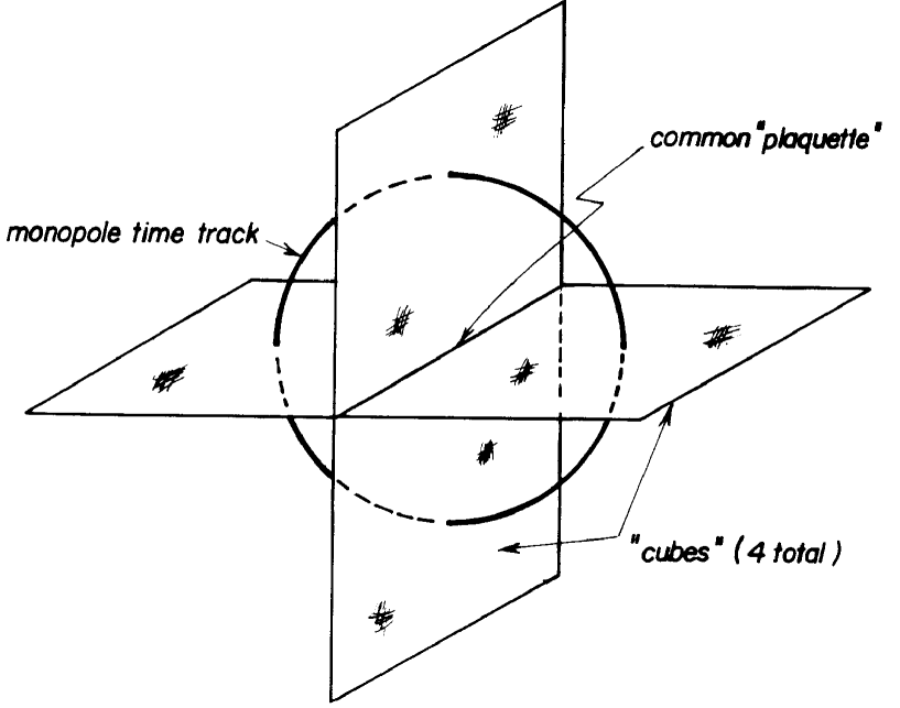
Figure 4: The important monopoles are expected to be of minimal strength and to be found essentially only in the dominant configuration of four cubes surrounding a common plaquette. The dominant configuration is illustrated above in a picture having one dimension less than the actual (4-dimensional) dominant configuration. The actual dominant configuration - i.e., a plaquette common to four 3-cubes has in the above dimensionally reduced picture become a link common to four plaquettes.

We claim that as $\gamma\rightarrow\infty$, the probability of having such a dominant configuration monopole decreases exponentially; accordingly there is only a thin population of minimal “strength monopoles” (and an even much thinner population of monopoles other than the “minimal strength” type). Hence it is presumably a very good approximation to describe the presence of monopoles as due solely to the dominant configuration of “minimal strength” monopoles.

In the case of the action (75), this means four 3-cube $\frac{2\pi}{4\pi}$-monopoles that encircle a common plaquette having a value corresponding to the nontrivial element of $\mbox{\bf{Z}}_{2}$. Consider by way of example the case where each of the four 3-cubes in this dominant configuration have the value $2\pi/5$ on five plaquettes (with the sixth “encircled” common plaquette having the value $\pm 2\pi$). Such a 3-cube configuration would, relative to a $\mbox{\bf{Z}}_{2}$ background flux (expected for large $\gamma$ and small $\beta$’s), behave as a $\frac{2\pi}{4\pi}$-monopole with a flux of $2\pi/5$ emanating from each of five plaquettes.

The dominant-configuration $\frac{2\pi}{4\pi}$-monopoles can be expected to occur with some low but nonzero density in the lattice near the phase border “2” even for large (but not too large) $\gamma$ values. Our suspicion, confirmed by calculations below, is that the degree of “first-orderness” of the phase transition at the boundary “2” is greater the smaller the chance that small deviations from $\mbox{\bf{Z}}_{2}$ (lying in $U(1)$) can, for the six plaquettes of a 3-cube, add up to a $\frac{2\pi}{4\pi}$-monopole (or, stated equivalently, add up to the length of the factor group $U(1)/\mbox{\bf{Z}}_{2}$).

As $\gamma$ decreases, an increasing number of $\frac{2\pi}{4\pi}$-monopoles is encountered. At the triple point (TP), where $\gamma\approx 1$, the presence of a larger number of $\frac{2\pi}{4\pi}$-monopoles than for very large $\gamma$ mitigates but does not eliminate the high degree of “first-orderness” characteristic of pure $\mbox{\bf{Z}}_{2}$ transitions (for which the deviations from $\mbox{\bf{Z}}_{2}$ (along $U(1)$) of six 3-cube plaquette variable values cannot sum to the length of the whole $U(1)/\mbox{\bf{Z}}_{2}$ due to $\gamma$ being too large).

In order to deal quantitatively with the effect of $\frac{2\pi}{4\pi}$-monopoles, and thereby with the question of how much of the behaviour of a pure $\mbox{\bf{Z}}_{2}$ transition is inherited by the phase transition at border “2” at the triple point, it is useful to define two new variables $U_{sign\;U(\Box)}(\Box)$ and $U_{BIO}(\Box)$:

$$U_{sign\;U(\Box)}(\Box)\stackrel{{\scriptstyle def}}{{=}}\left\{\begin{array}[]{l}+1\mbox{ if $U(\Box)$ closest to $e^{i0}\in\mbox{\bf{Z}}_{2}$}\\ -1\mbox{ if $U(\Box)$ closest to $e^{i\pi}\in\mbox{\bf{Z}}_{2}$}\end{array}\right.$$ (96)

The other new variable $U_{BIO}(\Box)$ (the subscript “$BIO$” is an acronym for Bianchi Identity Obeying) is defined as follows:

$$U_{BIO}(\Box)\stackrel{{\scriptstyle def}}{{=}}U_{sign\;U(\Box)}(\Box)\cdot$$ (97)

$$\cdot\left\{\begin{array}[]{l}+1\mbox{ \footnotesize for ordinary $\Box$ (i.e. {\em not} the encircled $\Box$ in the dominant config.)}\\ -1\mbox{ \footnotesize for $\Box$ encircled by four 3-cube $\frac{2\pi}{4\pi}$-monopoles in the dominant config.}\end{array}\right.$$

The variable $U_{BIO}(\Box)$ differs from the variable $U_{sign\;U(\Box)}(\Box)$ only by a sign change of $U_{sign\;U(\Box)}(\Box)$ in the case where the plaquette $\Box$ coincides with the “encircled” plaquette. The “encircled” plaquette is always present in the four 3-cube $\frac{2\pi}{4\pi}$-monopoles of the dominant monopole configuration.

Let us make the observation that the values assigned by the variable $U_{sign\;U(\Box)}(\Box)$ to the plaquettes of a 3-cube satisfy the $\mbox{\bf{Z}}_{2}$-Bianchi identity if the 3-cube is not a $\frac{2\pi}{4\pi}$-monopole; i.e., in our approximation, not one of the four 3-cube $\frac{2\pi}{4\pi}$-monopoles encircling a common plaquette in the dominant $\frac{2\pi}{4\pi}$-monopole configuration. Note, however, that the Bianchi identity is violated by the values assigned by the variable $U_{sign\;U(\Box)}(\Box)$ to the plaquettes of a 3-cube when there is a $\frac{2\pi}{4\pi}$-monopole. For instance, it is readily seen that for the very special $\frac{2\pi}{4\pi}$-monopole example given above ($U(\Box)=e^{i\frac{2\pi}{4\pi}\cdot 2\pi}=-1$ on the “encircled” plaquette; $U(\Box)=e^{i2\pi/5}$ on the remaining 5 plaquettes of the $\frac{2\pi}{4\pi}$-monopole 3-cube), the Bianchi identity is violated:

$$\prod_{\Box\in\partial(\frac{2\pi}{4\pi}-monopole\;3-cube)}U_{sign\;U(\Box)}(\Box)=(-1)\cdot 1^{5}=-1\neq 1$$ (98)

inasmuch as $U_{sign\;U(\Box)}(\Box)=-1$ for $U(\Box)=-1$ and $U_{sign\;U(\Box)}(\Box)=1$ for $U(\Box)=e^{i2\pi/5}$.

More generally, a $\frac{2\pi}{4\pi}$-monopole (which really just means a monopole modulo a $\mbox{\bf{Z}}_{2}$ background) consists of a configuration of plaquette variable values of a 3-cube that deviate continuously from elements of $\mbox{\bf{Z}}_{2}$ in such a way that the total sum of continuous deviations (lying in $U(1)$) from $\mbox{\bf{Z}}_{2}$ equals, modulo $4\pi$, $2\pi$ multiplied by the number of plaquettes for which the continuous deviations are centred at the nontrivial element of $\mbox{\bf{Z}}_{2}$. Note that in order to have a monopole, an odd number of the six plaquettes of a three cube must be near the nontrivial element (i.e., $2\pi$) of $\mbox{\bf{Z}}_{2}$

Even more generally, we have for a monopole modulo a $\mbox{\bf{Z}}_{N}$ background (i.e., a monopole for which the continuous $U(1)$ deviations from $Z_{N}\subset U(1)$ add up to a multiple of the length of the factor group $U(1)/\mbox{\bf{Z}}_{N}$):

$$\prod_{\mbox{\tiny$\Box\in$ 3-cube}}(U(\Box)g_{{}_{\tiny nearest}}(U(\Box))^{-1})=\prod_{\mbox{\tiny$\Box\in$ 3-cube}}g_{\tiny nearest}(U(\Box))\;\;\;\;\;\;\;(g_{\tiny nearest}(U(\Box))\in\mbox{\bf{Z}}_{N})$$ (99)

where $g_{\tiny nearest}(U(\Box))$ is defined as that element of $\mbox{\bf{Z}}_{N}$ which is nearest to $U(\Box)$:

$$dist^{2}(U(\Box),g_{\tiny\;nearest}(U(\Box)))\stackrel{{\scriptstyle def}}{{=}}inf\{dist^{2}(U(\Box),g^{\prime})\}\;\;\;\;(g^{\prime}\in\mbox{\bf{Z}}_{N})$$ (100)

where $dist^{2}(U(\Box),g^{\prime})$ denotes the squared distance from a plaquette variable value $U(\Box)$ and an element $g^{\prime}\in\mbox{\bf{Z}}_{N}$. We are really interested in $\mbox{\bf{Z}}_{6}=\mbox{\bf{Z}}_{2}\times\mbox{\bf{Z}}_{3}$ inasmuch as we are also interested in the modification of first-orderness due to an increasing number of monopoles modulo $\mbox{\bf{Z}}_{3}$ in going from large $\gamma$ to the triple point. However, for the purpose of exposition, we continue to use the example of monopoles modulo $\mbox{\bf{Z}}_{2}$.

With the modification of the variable $U_{sign\;U(\Box)}(\Box)$ that defines the variable $U_{BIO}(\Box)$, we have in $U_{BIO}(\Box)$ a variable that, for sufficiently large $\gamma$, assigns values to configurations of plaquettes that respects the $\mbox{\bf{Z}}_{2}$ Bianchi identities - also for $\frac{2\pi}{4\pi}$-monopole configurations (when the monopoles are of the dominant configuration type which is the only type for which the variable $U_{BIO}(\Box)$ is defined).

Note that the variable $U_{BIO}(\Box)$ differs from the variable $U_{sign\;U(\Box)}(\Box)$ only if there are $\frac{2\pi}{4\pi}$-monopoles. For $\gamma\rightarrow\infty$ such monopoles disappear and $U_{BIO}(\Box)=U_{sign\;U(\Box)}(\Box)\in\mbox{\bf{Z}}_{2}=\{+1,-1\}$. In going to smaller values of $\gamma$ in the phase with only $Z_{2}$ confining, an increasing range of fluctuations along $U(1)$ centred at the elements of $\{0,2\pi\}=\mbox{\bf{Z}}_{2}\subset U(1)$ provide alternative (Bianchi identity-obeying) configurations that supplement the essentially discrete group-valued plaquettes characteristic of large $\gamma$ configurations.

We want now to determine approximately the ($\gamma$ dependent) relation between the distributions of the two variables $U_{sign\;U(\Box)}(\Box)$ and $U_{BIO}(\Box)$. The average value of $U_{sign\;U(\Box)}(\Box)$ is estimated using the identity

$$\langle U_{sign\;U(\Box)}(\Box)\rangle=P(U_{BIO}(\Box)=+1)\langle U_{sign\;U(\Box)}(\Box)\rangle_{(U_{BIO}(\Box)=+1)}+$$ (101)

$$+P(U_{BIO}(\Box)=-1)\langle U_{sign\;U(\Box)}(\Box)\rangle_{(U_{BIO}(\Box)=-1)}$$

where $P(U_{BIO}(\Box)=+1)$ and $P(U_{BIO}(\Box)=-1)$ denote respectively the probabilities that $U_{BIO}(\Box)=+1$ and $U_{BIO}(\Box)=-1$ while $\langle U_{sign\;U(\Box)}(\Box)\rangle_{U_{BIO}(\Box)=+1}$ and $\langle U_{sign\;U(\Box)}(\Box)\rangle_{U_{BIO}(\Box)=-1}$ denote averages of $U_{sign\;U(\Box)}(\Box)$ subject respectively to the constraints that $U_{BIO}(\Box)=+1$ and $U_{BIO}(\Box)=-1$.

Denoting by $\xi=\xi(\gamma)$ the ($\gamma$ dependent) probability that a plaquette coincides with the “encircled plaquette” of the dominant $\frac{2\pi}{4\pi}$-monopole configuration, there obtains

$$\langle U_{sign\;U(\Box)}(\Box)\rangle_{U_{BIO}(\Box)=+1}=\frac{e^{\beta}\cdot 1+\xi e^{-\beta}\cdot(-1)}{e^{\beta}+\xi e^{-\beta}}$$ (102)

and

$$\langle U_{sign\;U(\Box)}(\Box)\rangle_{U_{BIO}(\Box)=-1}=\frac{e^{-\beta}\cdot(-1)+\xi e^{\beta}\cdot(+1)}{e^{-\beta}+\xi e^{\beta}}$$ (103)

Using

$$P(U_{BIO}(\Box)=+1)=\frac{1}{2}+\frac{1}{2}\langle U_{BIO}(\Box)\rangle$$ (104)

and

$$P(U_{BIO}(\Box)=-1)=\frac{1}{2}-\frac{1}{2}\langle U_{BIO}(\Box)\rangle$$ (105)

we have

$$\langle U_{sign\;U(\Box)}(\Box)\rangle=\frac{1}{2}\left(\frac{e^{\beta}-\xi e^{-\beta}}{e^{\beta}+\xi e^{-\beta}}+\frac{\xi e^{\beta}-e^{-\beta}}{\xi e^{\beta}+e^{-\beta}}\right)+\frac{1}{2}\left(\frac{e^{\beta}-\xi e^{-\beta}}{e^{\beta}+\xi e^{-\beta}}-\frac{\xi e^{\beta}-e^{-\beta}}{\xi e^{\beta}+e^{-\beta}}\right)\langle U_{BIO}(\Box)\rangle$$ (106)

$$\approx\langle U_{BIO}(\Box)\rangle(1-2\xi\cosh 2\beta)+2\xi\sinh 2\beta$$ (107)

where in the last step we have used that $\xi$ is assumed to be small.

We want now to calculate the jump in (88) in going from the phase with only $\mbox{\bf{Z}}_{2}$ confining to the totally Coulomb phase at the the triple point. That is, we want $\Delta\gamma_{eff}$ along the boundary “2” in Figure 3 as a function of $\gamma$:

$$\Delta\gamma_{eff}=\Delta(\gamma+\langle\sigma\rangle\frac{\beta_{crit}(\gamma)}{4})=\Delta\langle\sigma\rangle\frac{\beta_{crit}(\gamma)}{4}=\frac{\beta_{crit}(\gamma)}{4}\Delta\langle U_{sign\;U(\Box)}(\Box)\rangle.$$ (108)

where we have made the identification $\langle\sigma\rangle=\langle U_{sign\;U(\Box)}(\Box)\rangle$. Substituting (107) into (108) we get

$$\frac{\beta_{crit}(\gamma)}{4}\Delta\langle U_{sign\;U(\Box)}(\Box)\rangle=\frac{\beta_{crit}(\gamma)}{4}\Delta\langle U_{BIO}(\Box)\rangle(1-2\xi\cosh 2\beta(\gamma))$$ (109)

In our approximative procedure we identify $\Delta\langle U_{BIO}(\Box)\rangle$ with the jump in $\Delta\langle S_{\Box}\rangle$ for a $\mbox{\bf{Z}}_{2}$ gauge theory since the phase transition “2” at the triple point is determined from the phase of $\mbox{\bf{Z}}_{2}$.

Let us define a parameter $\beta_{BIO}$ as the action parameter $\beta$ in a $Z_{2}$ gauge theory which optimally reproduces the distribution of the variables $U_{BIO}(\Box)$ in the $U(1)$ theory (with the mixed action (75)) by using an action of the form

$$S=\beta_{BIO}\sum_{\Box}U_{BIO}(\Box).$$ (110)

In other words, $\beta_{BIO}$ is defined such that

$$\langle U_{BIO}(\Box)\rangle_{\mbox{\tiny in }U(1)\mbox{\tiny theory with }S=S(\beta,\gamma)}=\langle U_{BIO}(\Box)\rangle_{{\mbox{\scriptsize\bf{Z}}}_{2}\mbox{ \tiny theory with}S=\beta_{BIO}\sum_{\Box}U_{BIO}(\Box)}$$ (111)

We now want to obtain $\beta_{BIO}$ as a function of $\beta$ and $\xi$ (and hereby $\gamma$ inasmuch as $\xi=\xi(\gamma)$) by equating the ratio of the probabilities

$$\frac{P(U_{BIO}(\Box)=1)}{P(U_{BIO}(\Box)=-1)}$$ (112)

for the two actions $S=S(\beta,\gamma)$ and $S_{BIO}=\beta_{BIO}\sum_{\Box}U_{BIO}(\Box)$:

$$\frac{\overbrace{e^{\beta}}^{U_{sign\;U(\Box)}(\Box)=+1}+\overbrace{\xi e^{-\beta}}^{U_{sign\;U(\Box)}(\Box)=-1}}{\underbrace{e^{-\beta}}_{U_{sign\;U(\Box)}(\Box)=-1}+\underbrace{\xi e^{\beta}}_{U_{sign\;U(\Box)}(\Box)=+1}}=\frac{e^{\beta_{BIO}}}{e^{-\beta_{BIO}}}.$$ (113)

This procedure for estimating $\beta_{BIO}$ is somewhat errant in that Bianchi identities are ignored on both sides of equation (113) in various ways: first in the calculation of the ratio (112) and second, and presumably less importantly, in the simulation-by a-$\mbox{\bf{Z}}_{2}$ theory that defines $\beta_{BIO}$. The hope is that these error roughly cancel inasmuch as the same error is present on both sides of the equation.

Taking the logarithm of both sides of (113) and solving for $\beta_{BIO}$ yields

$$\beta_{BIO}=\beta+\frac{1}{2}\log\frac{1+\xi e^{-2\beta}}{1+\xi e^{2\beta}}$$ (114)

We want to use (114) to relate $\beta_{BIO}$ and $\beta_{crit}(\gamma)$ along the boundary “2” in Figure 3. Using that $\xi<<e^{\beta},\;1$ there obtains

$$\beta_{crit\;BIO}\approx\beta_{crit}(\gamma)+\frac{1}{2}\xi(e^{-2\beta}-e^{2\beta})=\beta_{crit}(\gamma)-\xi\sinh 2\beta.$$ (115)

Substituting (115) for $\beta_{crit}(\gamma)$ on the right-hand side of (109) yields

$$\Delta\gamma_{eff}=\frac{\beta_{crit}(\gamma)}{4}\Delta\langle U_{sign\;U(\Box)}(\Box)\rangle=\frac{1}{4}\beta_{crit\;BIO}\left(1+\frac{\xi\sinh 2\beta}{\beta_{BIO}}\right)\Delta\langle U_{BIO}(\Box)\rangle(1-2\xi\cosh 2\beta)=$$ (116)

$$=\frac{1}{4}\beta_{crit\;BIO}\Delta\langle U_{BIO}(\Box)\rangle\left(1+\xi\left(\frac{\sinh 2\beta}{\beta_{crit\;BIO}}-2\cosh 2\beta\right)\right).$$ (117)

Solving (115) for $\xi$ and substituting into (117) yields

$$\Delta\gamma_{eff}=\frac{1}{4}\beta_{crit\;BIO}\Delta\langle U_{BIO}(\Box)\rangle\left(1+(\beta_{crit}(\gamma)-\beta_{crit\;BIO})\left(\frac{1}{\beta_{crit\;BIO}}-\frac{2}{\tanh 2\beta}\right)\right).$$ (118)

From the literature [28] we have values for $\langle S_{\Box}\rangle_{{\mbox{\scriptsize\bf{Z}}}_{2}}=\Delta\langle U_{BIO}(\Box)\rangle$ and $\beta_{crit\;BIO}$. The quantity $\beta_{crit}(\gamma)-\beta_{crit\;BIO}$ is estimated graphically using a $U(1)$ phase diagram found in the literature[15] corresponding to the action (75). It is now finally possible to calculate $\Delta\gamma_{eff}$ at the triple point for the transition from the phase with only $\mbox{\bf{Z}}_{2}$ confining to the totally Coulomb-like phase.

It is indeed fortunate that the subtraction $\frac{1}{\beta_{BIO}}-\frac{2}{\tanh 2\beta}$ almost cancels thereby rendering our calculation of $\Delta\gamma_{eff}$ rather insensitive to the large uncertainty in the graphical estimate of $\beta_{crit}(\gamma)-\beta_{BIO}$. This means that the major contribution to the change in first-orderness in going from very large $\gamma$ to $\gamma\approx 1$ at the triple point is achieved simply by determining $\beta_{crit}(\gamma)$ by the condition that $\beta_{crit\;BIO}=\beta_{crit}(\gamma=\infty)$. This makes it possible to perform an analogous correction to the first-orderness in going from a pure $\mbox{\bf{Z}}_{3}$ theory to the triple point for an action $\gamma\cos\theta+\beta_{3}\cos\frac{\theta}{3}$ without having access to the phase diagram for the $U(1)$ theory with an action of this form (that we need for the graphical estimate of $\beta_{TP\;crit}(\gamma)-\beta_{{\mbox{\scriptsize\bf{Z}}}_{3}\;BIO}$).

In subsequent calculations, we shall make use of the fact that the probability $\xi$ of having a $\mbox{\bf{Z}}_{2}$ and a $\mbox{\bf{Z}}_{3}$ monopole must be roughly equal. The argument goes as follows: we can assume that essentially all monopoles present will be of the “minimal strength” type. In the case of the $SMG$, this means monopoles modulo a $\mbox{\bf{Z}}_{6}$ background: i.e., $\frac{2\pi}{12\pi}$-monopoles. These are built up of $U(1)$ elements close to $\mbox{\bf{Z}}_{6}$ such that the deviations from $\mbox{\bf{Z}}_{6}$ of six 3-cube plaquette variables add up to the full extent of $U(1)/\mbox{\bf{Z}}_{6}$. Of course it is still assumed that these “minimal strength” monopoles essentially only are found in dominant configuration of four 3-cubes that encircle a common plaquette But such a “minimal strength” monopole is a superposition of a $\mbox{\bf{Z}}_{2}$ and a $\mbox{\bf{Z}}_{3}$ monopole:

$$\frac{2\pi}{12\pi}=\frac{6\pi}{12\pi}-\frac{4\pi}{12\pi}$$ (119)

Assuming a rarity of $\pm\frac{2\pi}{4\pi}$-monopoles (i.e., $\pm\frac{6\pi}{12\pi}$-monopoles in the $12\pi$ normalisation) as well as $\frac{\pm 4\pi}{12\pi}$-monopoles (i.e., monopoles corresponding to the strength of a nontrivial element of the $\mbox{\bf{Z}}_{3}$ subgroup), monopoles are for all practical purposes exclusively of the $\frac{2\pi}{12\pi}$ type. And each of these “minimal strength” monopoles is formally a linear combination of exactly one $\mbox{\bf{Z}}_{2}$-monopole and one $\mbox{\bf{Z}}_{3}$-monopole. Hence these latter monopole types are “present” in essentially equal numbers.

As we would like to include not only the degree of first orderness inherited from $\mbox{\bf{Z}}_{2}$ at the triple point, but also that inherited from $\mbox{\bf{Z}}_{3}$, we need to generalise (108) and (117) which were derived for $\mbox{\bf{Z}}_{2}$ alone. The generalisation of (108) is obtained by varying (94):

$$\Delta\gamma_{eff}=\frac{\beta_{2}}{4}\Delta(\langle\sigma_{{\mbox{\scriptsize\bf{Z}}}_{2}}\rangle)+\frac{\beta_{3}}{9}\Delta(\langle\sigma_{{\mbox{\scriptsize\bf{Z}}}_{3}}\rangle)+\frac{\beta_{6}}{36}\Delta(\langle\sigma_{{\mbox{\scriptsize\bf{Z}}}_{6}}\rangle).$$ (120)

where the notation has been changed such that $\langle\sigma\rangle\stackrel{{\scriptstyle def}}{{=}}\langle U_{sign\;U(\Box)}(\Box)\rangle$ in (108) is in (120) denoted by $\langle\sigma_{{\mbox{\scriptsize\bf{Z}}}_{2}}\rangle$. For $\mbox{\bf{Z}}_{3}$ the analogous quantity is denoted by $\langle\sigma_{{\mbox{\scriptsize\bf{Z}}}_{3}}\rangle$ in (120). Moreover, we have the notational change $\beta_{crit\;BIO}\rightarrow\beta_{crit\;{\mbox{\scriptsize\bf{Z}}}_{2}}$ in going from (108) to (120). In (120) the analogous quantities for $\mbox{\bf{Z}}_{3}$ and $\mbox{\bf{Z}}_{6}$ are denoted respectively as $\beta_{crit\;{\mbox{\scriptsize\bf{Z}}}_{3}}$ and $\beta_{crit\;{\mbox{\scriptsize\bf{Z}}}_{6}}$. We have taken the $\beta_{6}$ term in (120) as being zero. This is presumably justified by the smallness of the $\mbox{\bf{Z}}_{6}$ “jump” contribution when treated (incorrectly) as being independent of $\mbox{\bf{Z}}_{2}$ and $\mbox{\bf{Z}}_{3}$.

In going to the new notation, (117) becomes (for $\mbox{\bf{Z}}_{2}$)

$$\Delta\gamma_{eff}=\frac{1}{4}\beta_{crit\;{\mbox{\scriptsize\bf{Z}}}_{2}}\Delta\langle S_{\Box}\rangle_{{\mbox{\scriptsize\bf{Z}}}_{2}}\left(1+\xi\left(\frac{\sinh 2\beta}{\beta_{crit\;{\mbox{\scriptsize\bf{Z}}}_{2}}}-2\cosh 2\beta\right)\right)$$ (121)

The generalisation that also includes the discontinuity inherited from $\mbox{\bf{Z}}_{3}$ that contributes to $\Delta\gamma_{eff}$ at the triple point transition from the phase with just the discrete subgroups $\mbox{\bf{Z}}_{2}$ and $\mbox{\bf{Z}}_{3}$ confining to the totally Coulomb-like phase is

$$\Delta\gamma_{eff}=\sum_{N\in\{2,3\}}\frac{1}{N^{2}}\beta_{crit\;{\mbox{\scriptsize\bf{Z}}}_{N}}\Delta\langle S_{\Box}\rangle_{{\mbox{\scriptsize\bf{Z}}}_{N}}\left(1+\xi\left(\frac{\sinh 2\beta}{\beta_{crit\;{\mbox{\scriptsize\bf{Z}}}_{N}}}-2\cosh 2\beta\right)\right).$$ (122)

From the argumentation above, we know that $\xi$ is expected to have the same value in both terms of (122).

In (122) it is seen that the subgroups $\mbox{\bf{Z}}_{2}$ and $\mbox{\bf{Z}}_{3}$ both contribute a term to $\Delta\gamma_{eff}$ at the triple point. Presumably it is a good approximation to calculate $\Delta\gamma_{eff}$ as if contributions from $\mbox{\bf{Z}}_{2}$ and $\mbox{\bf{Z}}_{3}$ are mutually independent inasmuch as these subgroups factorize at the multiple point. However, even in this approximation there will still be an indirect interaction between these subgroups via the continuum degrees of freedom in $U(1)$ and via the encircled plaquette in the dominant monopole configuration. Using (122), the contributions from $\mbox{\bf{Z}}_{2}$ and $\mbox{\bf{Z}}_{3}$ to $\Delta\gamma_{eff}$ are calculated and tabulated in Table 4.

Table 4: The quantity $\Delta\gamma_{eff}$ calculated using the appropriate terms in (122). In the last row, the quantities for $\mbox{\bf{Z}}_{6}$ are calculated (incorrectly) in a manner analogous to that used for $\mbox{\bf{Z}}_{2}$ and $\mbox{\bf{Z}}_{3}$. This procedure presumably overestimates the effect of $\mbox{\bf{Z}}_{6}$ contributions.

$$\begin{array}[]{|l|l|l|l|l|}\hline\cr&\beta_{crit\;{\mbox{\scriptsize\bf{Z}}}_{N}}&\Delta\langle S_{\Box}\rangle_{{\mbox{\scriptsize\bf{Z}}}_{N}}&\xi&\Delta\gamma_{eff}\\ \hline\cr\mbox{\bf{Z}}_{2}&0.44&0.44&0.04&0.047_{3}\\ \hline\cr\mbox{\bf{Z}}_{3}&0.67&0.56&0.04&0.039_{3}\\ \hline\cr(\mbox{\bf{Z}}_{6})&(1.00)&(0.13)&(0.0437)&(0.0033)\\ \hline\cr\end{array}$$ (123)

5.4 Calculating the enhancement factor for $1/\alpha_{U(1)}$ corresponding to the Planck scale breakdown of $U(1)^{3}$ to the diagonal subgroup

The two approximations that we have developed in order to gain an insight into the phase diagram for the group $U(1)^{3}$ - the independent monopole approximation and the group volume approximation - are more or less suitable according to whether the phase transitions are second or first order.

To determine the correct enhancement factor, we interpolate between the independent monopole approximation that gives this factor as 6 and the volume approximation that puts this factor at about 8. This interpolation is done by calculating the jump $\Delta W_{\Box\;``3"}$ in the Wilson operator at the boundary “3” transition at the TP (see Figure 3) that reflects the degree of first-orderness inherited at this transition from pure $\mbox{\bf{Z}}_{2}$ and $\mbox{\bf{Z}}_{3}$ transitions. As $\Delta\gamma_{eff}$ expresses the degree of first-orderness at the TP in going into the totally Coulomb-like phase, $\Delta W_{\Box\;``3"}$ is calculated using the assumption that it depends essentially on $\Delta\gamma_{eff}$.

The first approximation is the monopole condensate approximation in which the relevant quantity for which phase is realized is the amount of fluctuation in the convolution of the 6 plaquette variables enclosing a 3-cube.

In the second approximation - based on the group volume approximation - it turns out that to attain the multiple point in the hexagonal symmetry scheme, it is necessary to introduce additional parameters in the form of coefficients to 4$th$ and 6$th$ order perturbations to the Manton action. These additional parameters are used to get the free energy functions (corresponding to different phases) to coincide in parameter space at a point - “the” multiple point. This point is shared by what we expect is a maximum number of phases.

If, for example, the Coulomb to confining phase transition for a $Peter$-$U(1)$ subgroup is purely second order, this phase transition would not be expected to cause any change in at what value of the distance along another subgroup axis (e.g., the $Paul$-axis) the first identification-lattice point is encountered. The reason is that there is no discontinuous change in the degree of fluctuation in the $Peter$-plaquette variable in making the transition. In this case we expect the independent monopole approximation to work well.

On the other hand, if the phase transition is very strongly first order so that the fluctuations along the $Peter$-subgroup become discontinuously larger upon passing into the $Peter$ confinement phase, this can be expected to affect the threshold at which other subgroups go into confinement in a sort of “interaction effect”. In this situation the volume-approximation can be useful because it can take into account (and actually overestimates) the influence that fluctuations along different directions in the group can have on each other. The independent monopole approximation tends to ignore this effect.

Because the group volume approximation accounts for the interaction effect between fluctuations along different subgroups, it was necessary to use $4th$ and $6th$ order action terms in order to get a multiple point at which 12 phases convene (corresponding to continuous invariant subgroups; we neglect an infinity of discrete subgroups in this approximation). The effect of the higher order terms is the preferential enhancement of quantum fluctuations along the one dimensional (nearest neighbour) subgroup directions of the identification lattice thereby effectively eliminating the influence that fluctuations along one subgroup have on the fluctuations along another subgroup and vice versa.

In fact, the volume approximation effectively replaces the gauge group $G$ by its factor group $G/H$ when $H$ has confinement-like behaviour. This amounts to treating the fluctuations along the component of the group lying within the cosets $gH\;\;(g\in G)$ as being so large that, as far as Bianchi identities are concerned, we can regard the distribution of elements within the cosets of $H$ as essentially being that of the Haar measure .

5.4.1 The independent monopole condensate approximation - the calculation

In the independent monopole approximation, we can reach the multiple point using the Manton action alone (i.e., no higher order terms). The diagonal $U(1)$ subgroup to be identified with the $U(1)$ of the $SMG$ is that given by $\theta(1,1,1)$ in the coordinate choice (47).

The first identification lattice point met by this diagonal subgroup occurs for $\theta=2\pi$; i.e., the point $2\pi(1,1,1)$. Hence the quantisation rule $y/2\in{\bf Z}$ (for particles not carrying non-Abelian gauge coupling) is achieved by the naive continuum limit identification

$$\exp(i\theta(-))=\exp(iag_{1}A_{\mu}y/2)\;\;\;\mbox{for}\;\;\;y/2=1.$$ (124)

For $y/2=1$ (corresponding to $e^{+}_{L}$), the covariant derivative is

$$D_{\mu}=\partial_{\mu}-ig_{1}A_{\mu}.$$ (125)

The equation analogues to (40) for the diagonal subgroup (on the 3-dimensional identification lattice) is

$$\frac{\beta_{diag}}{2}(2\pi)^{2}=length(2\pi(1,1,1))=$$ (126)

$$=(2\pi)^{2}(1,1,1)\frac{\beta_{crit}}{2}\left(\begin{array}[]{ccc}1&\frac{1}{2}&\frac{1}{2}\\ \frac{1}{2}&1&\frac{1}{2}\\ \frac{1}{2}&\frac{1}{2}&1\end{array}\right)\left(\begin{array}[]{c}1\\ 1\\ 1\end{array}\right)=(2\pi)^{2}\frac{\beta_{crit}}{2}\cdot 6$$

for the multiple point. Contrary to the case of the non-Abelian couplings that are weakened by a factor $N_{gen}=3$ in going to the diagonal subgroup of $U(1)^{3}$, the $U(1)$ coupling at the multiple point is weakened by a factor 6 in going to the diagonal subgroup of $U(1)^{3}$. In general, the weakening factor in the hexagonal case in going from $U(1)^{N_{gen}}$ to the diagonal subgroup $U(1)$ along the direction $(1,1,\cdots,1)$ is $N_{gen}+\left(\begin{array}[]{c}N_{gen}\\ 2\end{array}\right)=N_{gen}(N_{gen}+1)/2$:

so that

$$g^{2}_{diag}=\frac{g^{2}_{crit}}{N_{gen}(N_{gen}+1)/2}.$$ (127)

5.4.2 The volume of groups scheme

In the earlier section 4.3.2, we have developed a means for calculating an effective inverse squared coupling having a directional dependence on $4th$ and $6th$ order action terms. We now calculate the effective inverse squared coupling (65) along the diagonal subgroup:

$$\frac{1}{e^{2}_{eff}(\vec{\xi})}\mbox{ (for $\xi=(1,1,1)$) }=$$ (128)

$$\left(B_{6}Y_{6\;\;comb}(diag)+\left(\frac{1}{e^{2}_{Manton}}+B_{4}Y_{4\;\;comb}(diag)\right)^{\frac{3}{2}}\right)^{\frac{1}{3}}=$$

$$=\left(\frac{-0.766}{e^{6}_{U(1)\;\;crit}}(-4\sqrt{\frac{3}{35}})+\left(\frac{2^{\frac{2}{3}}}{e^{4}_{U(1)\;\;crit}}+\frac{-0.146}{e^{4}_{U(1)\;\;crit}}\frac{2}{3}\sqrt{7}\right)^{\frac{3}{2}}\right)^{\frac{1}{3}}=$$

$$=1.34\cdot\frac{1}{e^{2}_{U(1)\;\;crit}}\;\;\;\mbox{ (in vol. approx.)}$$

From (126) we have that the inverse squared coupling corresponding to the diagonal subgroup of $U(1)^{3}$ is a factor 6 larger than $\frac{1}{e^{2}_{U(1)\;\;crit}}|_{\xi=(1,1,1)}\;$:

$$\frac{1}{e^{2}(diag)}=6\cdot\frac{1}{e^{2}_{eff}(\vec{\xi})}\left|{}_{\vec{\xi}=(1,1,1)}\right.=6\cdot 1.34=8.04$$ (129)

5.4.3 The calculation of the enhancement factor

We have seen that the enhancement factor $\frac{1/\alpha_{U(1)^{3}}}{1/\alpha_{U(1)}}$ has respectively the values 6.0 and $1.34\cdot 6.0$ according to whether the “independent monopole” or the “volume” approximation is used. These approximations tend respectively to ignore and to overestimate the dependence that fluctuations in one subgroup can have on which phase is realized along other subgroups or factor-groups. This interaction effect depends on the degree of first-orderness of the phase transition; this degree of first-orderness is used in our procedure to determine to what extent the pure “monopole approximation” should be “pushed” towards the “volume approximation”. We seek a combination of these two approximations - with the relative weight determined by the degree of first-orderness - that is to be embodied in the value of $\Delta\gamma_{eff}$ that subsequently is used in both steps of the calculation of the $U(1)$ continuum coupling. In this section, we use $\Delta\gamma_{eff}$ to determine the $U(1)$ coupling at the multiple point of a phase diagram for a $U(1)^{3}$ gauge group.

The correction for the degree of first-orderness will be implemented by choosing the “hop” $\Delta W=\Delta\langle\cos\theta\rangle$ in the Wilson operator at the TP transition to the totally Coulomb-like phase in such a way that it reflects the residual first-orderness. This transition obviously has to separate confinement-like and Coulomb-like phases for the continuum degrees of freedom. There are two possibilities - namely the TP transition at border “1” and the TP transition at border “3” corresponding let us say to respectively the jumps $\Delta W_{\Box\;TP\;``1"}$ and $\Delta W_{\Box\;TP\;``3"}$ in the Wilson operator.

But we now argue that $\Delta W_{\Box\;TP\;``1"}$ is not what we want because it doesn’t reflect the degree of “residual” first-orderness (at the TP) that is due to the $Z_{N}$ transition The reason has to do with $Z_{N}$ ($N=2,3$) being in the same phase on both sides of the border “1” at the TP. Accordingly, $\Delta W_{\Box\;TP\;``1"}$ cannot reflect the discrete group transition.

So it is the discontinuity $\Delta W_{\Box\;TP\;``3"}$ that we want to use to interpolate between the “independent monopole” and the “volume” approximation so as to obtain the enhancement factor $\frac{\alpha_{U(1)^{3}\;diag}}{\alpha_{U(1)\;crit}}$ that reflects the appropriate degree of first-orderness for the TP transition in going from confinement to Coulomb-like behaviour for the continuum degrees of freedom.

In order to estimate the residual “first-orderness” present at the multiple point in making the transition to the totally Coulomb-like phase from the phase(s) with confinement solely w.r.t to discrete subgroup(s), we shall use the already proposed scenario in which we speculate that the increased frequency of minimal strength monopoles (i.e., $\frac{2\pi}{4\pi}$ monopoles in the $4\pi$ normalisation implicit in (75)) is related to the fact that the phase transition along the border “2” in Figure 3 becomes less and less strongly first order as $\gamma$ decreases. That is, we speculate that the increasing role of minimal strength monopoles (in the $4\pi$ normalisation, the minimal strength $\frac{2\pi}{4\pi}$ monopoles are the only monopoles; in the $12\pi$ normalisation, there are, in addition to minimal and most abundant $\frac{2\pi}{12\pi}$ monopoles, also (less common) $\frac{6\pi}{12\pi}$- and $\frac{4\pi}{12\pi}$-monopoles) in typical plaquette configurations is the reason that the transitions to the totally Coulomb-like phase at border “2” and subsequently, also at border “3” in Figure 3 becomes less and less first order as $\gamma$ is diminished.

As mentioned just above, it is well known that, for $U(1)$, the phase transition at border “3” becomes second order at the tri-critical point (at a slightly negative value of $\gamma$) and continues as a second order phase transition for $\gamma$ values less than the tri-critical value $\gamma_{TCP}$. The above picture is not inconsistent with the results of numerical studies that clearly reveal even a pure $U(1)$ gauge theory with a Wilson action (i.e., a theory with $\gamma=0$) as having a weakly first order phase transition as evidenced by a “jump” $\Delta W_{\Box}$ in the Wilson operator $W_{\Box}$. Indeed one finds in the work of Jersàk[29] et al fits that relate the “jump” $\Delta W_{\Box}$ in the Wilson operator $W_{\Box}\stackrel{{\scriptstyle def}}{{=}}\langle\cos(\theta_{\Box})\rangle$ to $\Delta\gamma\stackrel{{\scriptstyle def}}{{=}}\gamma-\gamma_{TCP}$ where $\gamma_{TCP}$ denotes the value of $\gamma$ in the tri-critical point:

$$\Delta W_{\Box}=A(\gamma-\gamma_{TCP})^{\beta_{\mu}}$$ (130)

The values for $\gamma_{TCP}$ and $\beta_{\mu}$ are given respectively as $\gamma_{TCP}=-0.11\pm 0.05$ and $\beta_{\mu}=1.7\pm 0.2$ while the constant $A$ is deduced to be $A=0.68_{35}$. For $\gamma=0$ (corresponding to a Wilson action), there obtains $\Delta W_{\Box}=0.68(0.11)^{1.7}=0.016$.

Actually this latter discontinuity will be seen to be of interest to us because it can be shown that this jump is to a good approximation the jump $\Delta W_{\Box,\;``1"}$ encountered in crossing border “1” near the multiple point. The reasoning is as follows: the jump $\Delta W_{\Box,\;``1"}$ is to a good approximation constant along the phase border “1”; consequently, $\Delta W_{\Box,\;``1"}$ near the multiple point is essentially the same as that at $\gamma=1.01$ and $\beta=0$ which, in turn, is, by a simple change of notation, identical with the discontinuity $\Delta W_{\Box}$ at $\gamma=0$, $\beta=1.01$ that using (130) was found to have the value $\Delta W_{\Box}=0.016$.

So what is wanted for the purpose of calculating the enhancement factor is the jump $\Delta W_{\Box,\;``3"}$ encountered at the multiple point in traversing border “3” separating the totally Coulomb-like and totally confinement-like phases. What we have is a way to calculate $\Delta W_{\Box;\;``2"}$: this procedure relates $\Delta W_{\Box,\;``2"}$ to the cubic root[30, 31] of the quantity $\Delta\gamma_{eff}$ (see Section 5.3) encountered in crossing the border “2” at the multiple point. Were it not that the transition at border “1” is (weakly) first order but instead second order, then we would have had $\Delta W_{\Box,\;``1"}=0$ and

$$\Delta W_{\Box,\;``2"}=\Delta W_{\Box,\;``3"}=A(\Delta\gamma_{eff})^{\frac{1}{3}}\;\;\;\mbox{ (when $\Delta W_{\Box,\;``1"}=0$)}$$ (131)

where $A=0.252$. However, having argued that $\Delta W_{\Box,\;``1"}=0.16\neq 0$ corresponding to a weakly first order transition in crossing border “1” in the vicinity of the multiple point, we conclude on the grounds of continuity that this jump must be the difference in the “jumps” $\Delta W_{\Box,\;``2"}$ and $\Delta W_{\Box,\;``3"}$ in crossing respectively the borders “2” and “3” at the multiple point (see Figure 3). Recall that these jumps, observed in crossing the borders “2” and “3” near the multiple point are essentially assumed to be the residual effects of first-order pure discrete subgroup transitions at large $\gamma$. So in principle at least, the “jump” $\Delta W_{\Box;\;``3"}$ is obtained by correcting $\Delta W_{\Box\;``2"}$ (calculated by using (131)) by the amount of the “jump” $\Delta W_{\Box,\;``1"}$ in crossing border “1”. Using that $\Delta W_{\Box,\;``1"}$ is small, we make this correction in an approximate way by increasing $\Delta\gamma_{eff}$ in (131) by the corrective quantity

$$\Delta\gamma_{corr\;``1"}\stackrel{{\scriptstyle def}}{{=}}(\frac{\Delta W_{\Box,\;``1"}}{A})^{3}$$ (132)

obtained by inverting (131). In this approximation, we obtain

$$\Delta W_{\Box,\;``3"}\approx A(\Delta\gamma_{eff}+\Delta\gamma_{corr\;``1"})^{\frac{1}{3}}=$$ (133)

$$=A(\Delta\gamma_{eff}+(\frac{0.016}{0.252})^{3})^{\frac{1}{3}}$$

where we have used that $\Delta W_{\Box,\;``1"}=0.016$ in (132) which in turn has been used in (133). Strictly speaking, it is inconsistent to assume additivity in the “jumps” $\Delta W_{\Box,\;``1"}$, $\Delta W_{\Box,\;``2"}$, and $\Delta W_{\Box,\;``3"}$ (essential because of continuity requirements) and at the same time that both $\Delta W_{\Box,\;``2"}$ and $\Delta W_{\Box,\;``3"}$ are related to an appropriate $\gamma_{eff}$ by a cubic root law. Consistency requires $\Delta W_{\Box,\;``1"}=0$ corresponding to a second order transition. For small $\Delta W_{\Box,\;``1"}$, this inconsistency is not bothersome and the approximation (133) is good. In fact the corrective term $\Delta\gamma_{corr\;``1"}$ is so small so as not to yield a difference in $\Delta W_{\Box,\;``2"}$ and $\Delta W_{\Box,\;``3"}$ that is discernible to within the calculational accuracy.

Equation (133) provides a way of calculating the for us interesting $\Delta W_{\Box,\;``3"}$ at the multiple point. Various values of $\Delta W_{\Box,\;``3"}$ are tabulated in Table 5. These are calculated for different values of $\Delta\gamma_{eff}$ that in turn are obtained as combinations of the $\Delta\gamma_{eff}$ in Table 4 calculated for the $\mbox{\bf{Z}}_{2}$, $\mbox{\bf{Z}}_{3}$, and $\mbox{\bf{Z}}_{6}$ discrete subgroups of $U(1)$.

Before we use these various $\Delta W_{\Box,\;``3"}$ values to calculate the enhancement factor $\frac{\alpha_{U(1)^{3}\;diag}}{\alpha_{U(1)\;crit}}$, we need to develop a way of using the $\Delta W_{\Box,\;``3"}$ to interpolate between the “pure monopole” and the “volume” approximation. We now do this for the general case of any discontinuity $\Delta W_{\Box}$. In general, when there is a “jump” $\Delta W_{\Box}$, we estimate that we get the most correct enhancement factor $\frac{1/\alpha_{U(1)^{3}\;diag}}{1/\alpha_{U(1)}\;crit}$ by linearly interpolating between the enhancement factor “6” corresponding to the independent monopole approximation and the enhancement factor $1.34\cdot 6=8.04$ corresponding to the volume approximation. That is, the enhancement factor is calculated as

$$\left(\frac{1/\alpha_{U(1)^{3}\;diag}}{1/\alpha_{U(1)}}\right)_{actual}=\left(\frac{1/\alpha_{U(1)^{3}\;diag}}{1/\alpha_{U(1)}}\right)_{ind\;mono}+$$

$$+\frac{\eta}{\tau}\left[\left(\frac{1/\alpha_{U(1)^{3}\;diag}}{1/\alpha_{U(1)}}\right)_{vol}-\left(\frac{1/\alpha_{U(1)^{3}\;diag}}{1/\alpha_{U(1)}}\right)_{ind\;mono}\right]$$

$$=6+\frac{\eta}{\tau}[6(1.34-1)]$$ (134)

where $\frac{\eta}{\tau}$ is given by

$$\frac{\eta}{\tau}=\frac{\left(\frac{Coul\;fluc}{conf\;fluc}\right)^{2}_{ind\;\;mono}-\left(\frac{Coul\;fluc}{conf\;fluc}\right)^{2}_{actual}}{\left(\frac{Coul\;fluc}{conf\;fluc}\right)^{2}_{ind\;\;mono}-\left(\frac{Coul\;fluc}{conf\;fluc}\right)^{2}_{vol}}$$ (135)

and $\eta$ is defined as the numerator while $\tau$ the denominator on the right hand side of (135). Write

$$\left(\frac{Coul\;fluc}{conf\;fluc}\right)^{2}\stackrel{{\scriptstyle def}}{{=}}\frac{1-\langle\cos\theta\rangle_{Coul}}{1-\langle\cos\theta\rangle_{conf}}=1-\frac{\Delta W_{\Box}}{1-\langle\cos\theta\rangle_{conf}}$$ (136)

where in the last step we have used that $\langle\cos\theta\rangle_{Coul}=\langle\cos\theta\rangle_{conf}+\Delta W_{\Box}$.

Using that $\left(\frac{Coul\;fluc}{conf\;fluc}\right)^{2}_{ind\;mono}=1$ essentially by definition, we have using (135) and (136) that

$$\eta=\frac{\Delta W_{\Box}}{1-\langle\cos\theta\rangle_{conf}}=\Delta W_{\Box}/0.377$$ (137)

where in (137) we have used $\langle\cos\theta\rangle_{conf\;ph}=0.623$.

Various values of $\eta$ are tabulated in Table 5 corresponding to the values of $\Delta W_{\Box,\;``3^{\prime\prime}}$ that are also tabulated in the same Table.

The quantity $\frac{\eta}{\tau}$ are used to obtain the values for the enhancement factors $\frac{1/\alpha_{U(1)^{3}\;diag}}{1/\alpha_{U(1)}\;crit}$ tabulated in the final two columns of Table 5. The two columns correspond to $\frac{1/\alpha_{U(1)^{3}\;diag}}{1/\alpha_{U(1)}\;crit}$ for two different values of $\tau$. The first, corresponding to the roughest approximation, is for $\tau=1$ inasmuch as we make the approximation $\left(\frac{Coul\;fluc}{conf\;fluc}\right)^{2}_{vol}\approx 0$. The enhancement factors in the column at the extreme right hand side are obtained using a better estimate of $\tau$:

$$\tau=1-\left(\frac{Coul\;fluc}{conf\;fluc}\right)^{2}_{vol}=1-0.21=0.79.$$ (138)

The values of $\frac{1/\alpha_{U(1)^{3}\;diag}}{1/\alpha_{U(1)\;crit}}$ in the last column of Table 5 will appear in Table 6 in conjunction with the calculation of the Planck scale value of the continuum $U(1)$ fine-structure constant $1/\alpha_{U(1)\;Pl.\;scale}$.

Table 5: Enhancement factors given in the last four columns on the right are given for two ways of calculating $\tau$ as well as with and without $\Delta\gamma_{corr``1"}$ included in the calculation of $\Delta W_{\Box}$ in (133). For the quantity $\tau\stackrel{{\scriptstyle def}}{{=}}1-\left(\frac{Coul\;fluc}{conf\;fluc}\right)^{2}$ we have $\tau=1$ when confinement fluctuations are taken as infinite and $\tau=0.79$ when confinement fluctuations are taken as finite. The second and third columns contain $\Delta W_{\Box}$ calculated respectively with and without the quantity $\Delta\gamma_{corr``1"}$ in (133). The values for $\Delta\gamma_{eff}$ in the first column are taken from Table 4. The quantity $\eta$ in the fourth and fifth columns is defined in (135) and calculated according to (137) with and without the quantity $\Delta\gamma_{corr``1"}$ in the expression (133) for $\Delta W_{\Box}$.

Procedure $$\Delta\gamma_{eff} \Delta W_{\Box,``3"} \eta \frac{1/\alpha_{{U(1)}^{3}_{``diag"}}}{1/\alpha_{{U(1)}_{``crit"}}} \Delta\gamma_{corr``1"} \Delta\gamma_{corr``1"} \Delta\gamma_{corr``1"} \Delta\gamma_{corr``1"}=0 \Delta\gamma_{corr``1"} =0 \Delta\gamma_{corr``1"} =0 \tau=0.79 \tau=1 \tau=0.79 \tau=1 \langle\cos\theta\rangle_{Coul}=0.65 \langle\cos\theta\rangle_{Coul}=0.65 \frac{1}{2} \mbox{\bf{Z}}_{2} \mbox{\bf{Z}}_{2}+\mbox{\bf{Z}}_{3} \frac{0.047_{3}}{2}+ \frac{1}{2}(\mbox{\bf{Z}}_{2}+\mbox{\bf{Z}}_{3}) +\frac{0.039_{3}}{2} \frac{0.047_{3}}{2} \frac{1}{2}\mbox{\bf{Z}}_{2}+\mbox{\bf{Z}}_{3} +0.039_{3}$$ from (133) from (137) from (134) with with with Vol Approx: Haar (ideal) () 1 8.04 Haar, compact () 0.79 8.04 Mean field 7.29 7.02 Ideal ind mono 0 0 1 6 6 No discrete 0 0.016 0 0.042₄ 0 6.11₀ 6.08₇ 6 6 subgroups Using only: 0.047₃ 0.091₃ 0.091₁ 0.24₂ 0.24₂ 6.62₅ 6.49₄ 6.62₄ 6.49₃ Using 0.047₃+ : 0.039₃ 0.11₂ 0.11₁ 0.29₆ 0.29₆ 6.76₄ 6.60₄ 6.76₄ 6.60₃ Using : 0.088₇ 0.088₅ 0.23₅ 0.23₅ 6.60₇ 6.48₀ 6.60₆ 6.47₉ Using : 0.10₀ 0.10₀ 0.26₆ 0.26₆ 6.68₈ 6.54₃ 6.68₇ 6.54₂

5.5 Continuum critical coupling from critical $U(1)$ lattice coupling

The Planck scale prediction for the $U(1)$ fine-structure constant is to be obtained as the product of the enhancement factor and the continuum critical coupling that corresponds to the lattice critical coupling.

We have the enhancement factor in Table 5 (calculated using different approximations) but we have yet to translate the lattice $U(1)$ critical coupling into a continuum one. This is the purpose of this section.

We use a procedure analogous to that used by Jersàk et al[18]. In this work the continuum coupling is calculated numerically. Using Monte Carlo methods on the lattice, the Coulomb potential is computed and fitted to the formula proposed by Luck ([27]). In the Coulomb phase with the Wilson action, the fit yields

$$Wilson:\;\;\;\alpha(\beta)=0.20-0.24(\frac{\beta-\beta_{crit}}{\beta})^{0.39}\;=\;0.20-0.24(1-\frac{1.0106}{\beta})^{0.39}.$$ (139)

For the Villain action (in the Coulomb phase) the analogous result is

$$Villain:\;\;\;\alpha(\beta)=0.20-0.33(1-\frac{0.643}{\beta})^{0.52}.$$ (140)

It is of course our intention to substitute $\gamma_{eff}$ for what Jersak et al. designates as $\beta$. This is justified in as much as (139) is valid for $\beta\geq\beta_{crit}$; i.e., for $\beta$ lying within the Coulomb phase. The replacement of

$$\beta-\beta_{crit}$$ (141)

by

$$\gamma_{eff\;tot\;Coul\;ph}-\gamma_{eff.\;only\;{\mbox{\scriptsize\bf{Z}}}_{2}\;conf}\stackrel{{\scriptstyle def}}{{=}}\Delta\gamma_{eff}$$ (142)

is valid inasmuch as the phases separated by the phase boundary “2” in Figure 3 are both in the Coulomb phase as far as the continuum degrees of freedom are concerned. Values obtained for $\alpha$ using (139) with $\beta$ replaced by $\gamma_{eff}$ and $\beta-\beta_{crit}$ by $\Delta\gamma_{eff}$ are tabulated for various values of the latter in the third column of Table 6.

Table 6: Our Planck scale prediction for the $U(1)$ fine-structure constant is obtained as the product of the enhancement factor (from the last four columns of Table (5)) and the value of $1/\alpha_{cont}$ obtained from the critical value of the lattice parameter $\gamma_{eff}$ and the “jump” $\Delta\gamma_{eff}$ in this same quantity in crossing the phase border “3” (see Figure 3) at the multiple point. We list a number of combinations that differ according to how the discrete subgroups are treated w.r.t. whether the discrete subgroups are large enough to have the symmetry of the hexagonal identification lattice and how $\tau$ (see Table 5) is calculated as an indication of the sensitivity of our prediction to such details. The prediction marked with “$\bullet$” indicates the predicted value calculated in what we regard as the most correct manner. Also included are results for the Villian action where (140) has been used to calculate $\alpha(\beta)$. In this table, we use the same $\Delta\gamma_{eff}$ in both (139) and (140) (this is incorrect; see next table). In the Villian case, the $\Delta W_{\Box\;``3"}$ used in calculating the enhancement factor is calculated as $\Delta W_{\Box\;``3"}=0.16(\Delta\gamma_{eff})^{0.29}$ (this is the counterpart of (133) for the Wilson action) with $\Delta_{``1"\;corr}=0$). The coefficient “0.16” is estimated from Monte Carlo data in ([18]) and is rather uncertain.

$$\!\!\!\!\!\!\!\!\!\!\!\!\begin{array}[]{|l|l|l|l|l|l|l|l|}\hline\cr\vrule\lx@intercol\hfil\mbox{single $U(1)$}\hfil\lx@intercol\vrule\lx@intercol\\ \hline\cr\mbox{Procedure}&\Delta\gamma_{eff}&\alpha_{cont.}&1/\alpha_{cont.}&\lx@intercol\hfil\mbox{enh. fac Haar}\hfil\lx@intercol\vrule\lx@intercol&\lx@intercol\hfil\mbox{prediction $1/\alpha_{Pl.scale}$}\hfil\lx@intercol\vrule\lx@intercol\\ \cline{5-8}\cr&&&&\tau=0.79&\tau=1&\tau=.79&\tau=1\\ \hline\cr\mbox{Wilson action (using (\ref{contfor}))}&&&&&&&\\ \hline\cr\mbox{$\mbox{\bf{Z}}_{2}$ only with $\Delta\gamma_{corr``1"}$ in (\ref{jump3})}&0.047_{3}&0.128_{6}&7.77_{8}&6.62_{5}&6.49_{4}&51.5&50.5\\ \hline\cr\mbox{$\mbox{\bf{Z}}_{2}$ only without $\Delta\gamma_{corr``1"}$ in (\ref{jump3})}&0.047_{3}&0.128_{6}&7.77_{8}&6.62_{4}&6.49_{3}&51.5&50.5\\ \hline\cr\mbox{$\mbox{\bf{Z}}_{2}+\mbox{\bf{Z}}_{3}$ with $\Delta\gamma_{corr``1"}$ in (\ref{jump3})}&0.086_{6}&0.110_{8}&9.02_{1}&6.76_{4}&6.60_{4}&61.0&59.6\\ \hline\cr\mbox{$\mbox{\bf{Z}}_{2}+\mbox{\bf{Z}}_{3}$ without $\Delta\gamma_{corr``1"}$ in (\ref{jump3})}&0.086_{6}&0.110_{8}&9.02_{1}&6.76_{4}&6.60_{3}&61.0&59.6\\ \hline\cr\mbox{$\frac{1}{2}(\mbox{\bf{Z}}_{2}+\mbox{\bf{Z}}_{3})$ with $\Delta\gamma_{corr``1"}$ in (\ref{jump3} )}&0.043_{3}&0.130_{9}&7.64_{0}&6.60_{7}&6.48_{0}&50.5&49.5\\ \hline\cr\mbox{$\frac{1}{2}(\mbox{\bf{Z}}_{2}+\mbox{\bf{Z}}_{3})$ without $\Delta\gamma_{corr``1"}$ in (\ref{jump3})}&0.043_{3}&0.130_{9}&7.64_{0}&6.60_{6}&6.47_{9}&50.5&49.5\\ \hline\cr\mbox{$\frac{1}{2}\mbox{\bf{Z}}_{2}+\mbox{\bf{Z}}_{3}$ with $\Delta\gamma_{corr``1"}$ in (\ref{jump3})}&0.063_{0}&0.120_{6}&8.29_{2}&6.68_{9}&6.54_{3}&55.5\;\;\bullet&54.3\\ \hline\cr\mbox{$\frac{1}{2}\mbox{\bf{Z}}_{2}+\mbox{\bf{Z}}_{3}$ without $\Delta\gamma_{corr``1"}$ in (\ref{jump3})}&0.063_{0}&0.120_{6}&8.29_{2}&6.68_{7}&6.54_{2}&55.5\;\;\bullet&54.3\\ \hline\cr\hline\cr\mbox{Villian action (using (\ref{vil}))}&&&&&&&\\ \hline\cr\mbox{$\mbox{\bf{Z}}_{2}$ only}&0.047_{3}&0.11_{8}&8.46_{5}&6.45_{2}&6.35_{7}&54.6&53.8\\ \hline\cr\mbox{$\mbox{\bf{Z}}_{2}+\mbox{\bf{Z}}_{3}$}&0.086_{6}&0.091_{1}&10.9_{8}&6.53_{9}&6.42_{6}&71.8&70.6\\ \hline\cr\mbox{$\frac{1}{2}(\mbox{\bf{Z}}_{2}+\mbox{\bf{Z}}_{3})$}&0.043_{3}&0.12_{2}&8.22_{6}&6.44_{1}&6.34_{8}&53.0\;\;\bullet&52.2\\ \hline\cr\mbox{$\frac{1}{2}\mbox{\bf{Z}}_{2}+\mbox{\bf{Z}}_{3}$}&0.063_{0}&0.10_{6}&9.42_{4}&6.49_{1}&6.38_{8}&61.2\;\;\bullet&60.2\\ \hline\cr\end{array}$$ (143)

The $\gamma_{eff}$ used in Table 6 is that calculated in (88) to lowest order in $\hat{\theta}$. We want now to go to next order in $\hat{\theta}$. For the Wilson action suitable for having a phase confined solely w.r.t. $\mbox{\bf{Z}}_{2}$, the appropriate effective coupling is given by (87). We denote this improved effective coupling by $\gamma_{eff\;corr}$:

$$\gamma_{eff\;corr}=\gamma+\frac{\langle\sigma_{\mbox{\bf{Z}}_{2}}\rangle_{\hat{\theta}}\beta}{4}\langle\frac{\cos(\hat{\theta}/2)}{\cos\hat{\theta}}\rangle\approx\gamma+\frac{\langle\sigma_{\mbox{\bf{Z}}_{2}}\rangle_{\hat{\theta}}\beta}{4}\langle\cos^{-\frac{3}{4}}\hat{\theta}\rangle\mbox{ (Wilson action)}.$$ (144)

The analogous improved $\gamma_{eff\;corr}$ for the Villian action case has the $\cos\hat{\theta}$ in the denominator in the average on the left-hand side of (144) removed corresponding to the Villian action being approximately a Manton action (having a second derivative that is $\hat{\theta}$-independent) instead of being equal to $\cos\hat{\theta}$ as in the Wilson case. So for the Villian action we have

$$\gamma_{eff\;corr}=\gamma+\frac{\beta}{4}\langle\sigma_{\mbox{\bf{Z}}_{2}}\rangle\cdot\langle\cos(\hat{\theta}/2)\rangle\approx\gamma+\frac{\beta}{4}\langle\sigma_{\mbox{\bf{Z}}_{2}}\rangle\cdot\langle\cos^{\frac{1}{4}}\hat{\theta}\rangle\;\;\;\mbox{(Villian action)}.$$ (145)

The effective couplings (144) and (145) are for respectively the Wilson and Villian actions. In both cases there can be a phase confined solely w.r.t. $\mbox{\bf{Z}}_{2}$. The analogous couplings for the Wilson and Villian actions in the case where there is a phase confined solely w.r.t. $\mbox{\bf{Z}}_{3}$ are given respectively by (146) and (147) below; i.e., by

$$\gamma_{eff\;corr}=\gamma+\frac{\beta}{9}\langle\sigma_{\mbox{\bf{Z}}_{3}}\rangle\langle\cos^{-\frac{8}{9}}\hat{\theta}\rangle\mbox{ (Wilson action)}$$ (146)

and

$$\gamma_{eff\;corr}=\gamma+\frac{\beta}{9}\langle\sigma_{\mbox{\bf{Z}}_{3}}\rangle\cdot\langle\cos^{\frac{1}{9}}\hat{\theta}\rangle\;\;\;\mbox{(Villian action)}.$$ (147)

Table 7: Here we use the improved effective couplings $\gamma_{eff\;corr}$ in (144) and (145) corresponding respectively to Wilson and Villian actions for which there is a phase confined solely w.r.t. $\mbox{\bf{Z}}_{2}$. The analogous improved effective couplings (146) and (147) are used respectively for the Wilson and Villian actions that can provoke phases confined solely w.r.t. $\mbox{\bf{Z}}_{3}$. Strictly speaking, for the improved calculation of $\Delta\gamma_{eff}$ - i.e., $\Delta\gamma_{eff\;corr}$ - we should (for say the Wilson action in the case where we have a phase confined solely w.r.t $\mbox{\bf{Z}}_{2}$) calculate as follows: $\Delta\gamma_{eff\;corr}=\frac{\beta}{4}\left(\langle\sigma\rangle_{Coul}\left\langle\frac{\cos\frac{\hat{\theta}}{2}}{\cos\hat{\theta}}\right\rangle_{Coul}-\langle\sigma\rangle_{conf}\left\langle\frac{\cos\frac{\hat{\theta}}{2}}{\cos\hat{\theta}}\right\rangle_{conf}\right)$ but because $\langle\sigma\rangle_{conf}<<\langle\sigma\rangle_{Coul}$ we have $\Delta\gamma_{eff\;corr}\approx\frac{\beta}{4}\left(\langle\sigma\rangle_{Coul}\left\langle\frac{\cos\frac{\hat{\theta}}{2}}{\cos\hat{\theta}}\right\rangle_{Coul}\right).$ We calculate $\Delta\gamma_{eff\;corr}$ iteratively inasmuch as the latter is needed to get $\Delta W$ which is needed to get $\langle\cos\hat{\theta}\rangle$ which in turn is needed to calculate $\Delta\gamma_{eff\;corr}$. The $\Delta W$ obtained iteratively using $\Delta\gamma_{eff\;corr}$ is also used in calculating the enhancement factor in Table 7. In the case of the Villian action, the cos$\hat{\theta}$ in the denominator of $\left\langle\frac{\cos\frac{\hat{\theta}}{2}}{\cos\hat{\theta}}\right\rangle$ is removed. The case having a phase confined solely w.r.t. $\mbox{\bf{Z}}_{3}$ is calculated in a way analogous to that for $\mbox{\bf{Z}}_{2}$ for respectively the Wilson and Villian action cases.

$$\!\!\!\!\!\!\!\!\!\!\!\!\!\!\!\begin{array}[]{|l|l|l|l|l|l|l|l|}\hline\cr\vrule\lx@intercol\hfil\mbox{single corrected $U(1)$ }\hfil\lx@intercol\vrule\lx@intercol\\ \hline\cr\mbox{Procedure}&\Delta\gamma_{eff,\;corr}&\alpha_{cont.}&1/\alpha_{cont.}&\lx@intercol\hfil\mbox{enh. factor Haar}\hfil\lx@intercol\vrule\lx@intercol&\lx@intercol\hfil\mbox{prediction $1/\alpha_{Pl.scale}$}\hfil\lx@intercol\vrule\lx@intercol\\ \cline{5-8}\cr&&&&\tau=0.79&\tau=1&\tau=0.79&\tau=1\\ \hline\cr\mbox{Wilson action (using (\ref{contfor}))}&&&&&&&\\ \hline\cr\mbox{$\mbox{\bf{Z}}_{2}$ only with $\Delta\gamma_{corr``1"}$ in (\ref{jump3})}&0.060_{0}&0.122_{0}&8.19_{6}&6.67_{7}&6.53_{5}&54.7&53.6\\ \hline\cr\mbox{$\mbox{\bf{Z}}_{2}+\mbox{\bf{Z}}_{3}$ with $\Delta\gamma_{corr``1"}$ in (\ref{jump3})}&0.109_{4}&0.103_{1}&9.69_{7}&6.82_{6}&6.65_{3}&66.2&64.5\\ \hline\cr\mbox{$\frac{1}{2}(\mbox{\bf{Z}}_{2}+\mbox{\bf{Z}}_{3})$ with $\Delta\gamma_{corr``1"}$ in (\ref{jump3} )}&0.0561_{5}&0.123_{9}&8.07_{2}&6.66_{2}&6.52_{3}&53.8\;\;\bullet&52.7\\ \hline\cr\mbox{$\frac{1}{2}\mbox{\bf{Z}}_{2}+\mbox{\bf{Z}}_{3}$ with $\Delta\gamma_{corr``1"}$ in (\ref{jump3})}&0.0810_{8}&0.112_{9}&8.85_{4}&6.74_{8}&6.59_{1}&59.7\;\;\bullet&58.4\\ \hline\cr\hline\cr\mbox{Villian action (using (\ref{vil}))}&&&&&&&\\ \hline\cr\mbox{$\mbox{\bf{Z}}_{2}$ only}&0.0431_{8}&0.121_{7}&8.21_{9}&6.44_{1}&6.34_{8}&52.9&52.2\\ \hline\cr\mbox{$\mbox{\bf{Z}}_{2}+\mbox{\bf{Z}}_{3}$}&0.0811_{9}&0.0942_{4}&10.6_{1}&6.52_{9}&6.41_{8}&69.3&68.1\\ \hline\cr\mbox{$\frac{1}{2}(\mbox{\bf{Z}}_{2}+\mbox{\bf{Z}}_{3})$}&0.0404_{4}&0.124_{1}&8.05_{5}&6.43_{2}&6.34_{1}&51.8\;\;\bullet&51.1\\ \hline\cr\mbox{$\frac{1}{2}\mbox{\bf{Z}}_{2}+\mbox{\bf{Z}}_{3}$}&0.0594_{1}&0.108_{7}&9.20_{4}&6.48_{3}&6.38_{2}&59.7\;\;\bullet&58.7\\ \hline\cr\end{array}$$ (148)

5.6 Results: Comparison of MPCP predictions with experimental values of fine-structure constants

Our Planck scale predictions for the gauge coupling constants come about as the product of the appropriate enhancement factor in going from the multiple point of $SMG^{3}$ to the diagonal subgroup and the continuum value of the lattice critical coupling.

In the case of the non-Abelian gauge couplings, the enhancement factor is just $N_{gen}=3$ whereas for the $U(1)$ coupling the enhancement factor is more than twice as large as in the non-Abelian case. Had the phase transition at the multiple point been purely second order, we would expect an enhancement factor of $\frac{1}{2}N_{gen}(N_{gen}-1)=6$ (instead of $N_{gen}=3$ as in the non-Abelian case) due to interaction terms of the type $F_{\mu\nu\;Peter}F^{\mu\nu}_{Paul}$ where the indices $Peter,Paul,\cdots$ label the various $SMG$ factors of $SMG^{N_{gen}}$ (of which there are $N_{gen}=3$). However, the fact that transitions between phases solely confined w.r.t. discrete subgroups and the totally Coulomb-like phase inherit a residual first-orderness of the pure discrete subgroup transitions leads to an enhancement factor larger than $\frac{1}{2}N_{gen}(N_{gen}-1)=6$. The enhancement factor for $U(1)$ is calculated using different approximations the result of which are tabulated in Table 5

The values we have calculated for the $U(1)$ gauge coupling (i.e., the values for the diagonal subgroup of $SMG^{3}$ at the multiple point of $SMG^{3}$) and the values calculated for the non-Abelian couplings are predicted to coincide with experimental values that have been extrapolated to the Planck scale using the assumption of a minimal standard model. In the renormalization group extrapolation procedure[32] used, we accordingly assume a desert with just a single Higgs ($N_{Higgs}=1$). The number of generations (families) is of course taken to be 3.

In doing the renormalization group extrapolation of experimental values to Planck scale, we start the running at the scale of $M_{Z}=91.176\pm 0.023$ using values from LEP experiments[33]. We also extrapolate the other way: we extrapolate our Planck scale predictions down to the scale of $M_{Z}$ so as these can be directly compared with experimental values of fine-structure constants. Predicted and experimental[32] values of the three fine-structure constants are compared at both the Planck scale and the scale of $M_{Z}$ are compared in Table 8. We have included predicted values obtained using several different variations in some details of our model. For the non-Abelian fine-structure constants, the naive continuum limit and the continuum-corrected continuum limit values are taken from our earlier work[4].

Table 8: Our predictions using slightly different calculational methods (approximations) and assumptions; these are compared with experimental values (Delphi results) extrapolated using the renormalization group to the Planck scale. The minimal Standard Model has been assumed in doing the extrapolation. The predicted values for $U(1)$ in the last eight rows are taken from Table 7 (with $\tau=0.79$).

SU(3)	$\alpha^{-1}(\mu_{Pl.})$	$\alpha^{-1}(M_{Z})$
Experimental values	53.6	9.25$\pm 0.43$
Continuum corrected continuum limit	$56.7\;\bullet$	12.${}_{8}\;\bullet$
Monopole correction	$56\pm 6\;\bullet$	$12._{1}\pm 6\;\bullet$
Naive continuum limit	$80._{1}$	$36._{2}$
SU(2)	$\alpha^{-1}(\mu_{Pl.})$	$\alpha^{-1}(M_{Z})$
Experimental values	49.2	30.10$\pm 0.23$
Continuum corrected continuum limit	$49.5\;\bullet$	29.${}_{8}\;\bullet$
Monopole correction	$48._{3}\pm 6\;\bullet$	$28._{5}\pm 6\;\bullet$
Naive continuum limit	$65._{1}$	$45._{3}$
U(1)	$\alpha^{-1}(\mu_{Pl.})$	$\alpha^{-1}(M_{Z})$
	($SU(5)$ norm. in parenthesis)	($SU(5)$ normalisation in parenthesis)
Experimental values:	54.8 (32.9)	98.70$\pm 0.21$ ($59.22\pm 0.13$)
Continuum corrected continuum limit	66 ($39._{6}$):	109.1 (65.5)
Naive continuum limit (w. enh. 6.8):	84.6(50.8)	127.7 (76.6)
Independent monopole approx.	30 (18)	73 (44)
$\mbox{\bf{Z}}_{2}$ (Wilson action):	54.7 (32.8)	97.8 (58.7)
$\mbox{\bf{Z}}_{2}$ (Villian action):	52.9 (31.7)	96.0 (57.6)
$\mbox{\bf{Z}}_{2}+\mbox{\bf{Z}}_{3}$ (Wilson action):	66.2 (39.7)	109.3 (65.6)
$\mbox{\bf{Z}}_{2}+\mbox{\bf{Z}}_{3}$ (Villian action):	69.3 (41.6)	112.4 (67.5)
$\frac{1}{2}(\mbox{\bf{Z}}_{2}+\mbox{\bf{Z}}_{3})$ (Wilson action):	53.8 (32.3)$\;\;\bullet$	96.9 (58.2)$\;\;\bullet$
$\frac{1}{2}(\mbox{\bf{Z}}_{2}+\mbox{\bf{Z}}_{3})$ (Villian action):	51.8 (31.1)$\;\;\bullet$	94.9 (57.0)$\;\;\bullet$
$\frac{1}{2}\mbox{\bf{Z}}_{2}+\mbox{\bf{Z}}_{3}$ (Wilson action):	59.7 (35.8)$\;\;\bullet$	102.8 (61.7)$\;\;\bullet$
$\frac{1}{2}\mbox{\bf{Z}}_{2}+\mbox{\bf{Z}}_{3}$ (Villian action):	59.7 (35.8)$\;\;\bullet$	102.8 (61.7)$\;\;\bullet$

6 Conclusion

We use the principle of multiple point criticality to calculate the values of the three standard model gauge couplings. These agree with experiment to well within the calculational accuracy of 5 to 10%. In the context used here, the principle states that Nature seeks out the action parameter values in the phase diagram of a lattice gauge theory that correspond to the multiple point. At this point, a maximum number of phases convene. The gauge group is taken as the $N_{gen}$-fold Cartesian product of the standard model group: $SMG^{N_{gen}}$ where $N_{gen}=3$ is the number of fermion generations. So there is a $SMG$ factor for each family of quarks and leptons. This gauge group is referred to as the Anti Grand Unified Theory $(AGUT)$ gauge group. At the Planck scale, the gauge couplings are predicted to have the multiple point values corresponding to the diagonal subgroup of $SMG^{N_{gen}}$. The diagonal subgroup, which is isomorphic to the usual standard model group, arises as that surviving the Planck scale breakdown of the more fundamental $SMG^{N_{gen}}$ under automorphic symmetry operations.

In order to provoke the many phase that should convene at the multiple point - including those corresponding to confinement solely of discrete subgroups of the gauge group - we need a rather general action the parameters of which span a multidimensional phase-diagram space. In many cases, such phases would be called lattice artifacts because the boundary between such lattice-scale phases disappears in going to long wavelengths and what is distinguishable as a Coulomb-like phase at lattice scales becomes indistinguishable from a confining phase at large distances. Such phases are usually regarded as not being of physical significance because they depend on the presence of a lattice which has been introduced only as a calculational regulator that must leave no trace of its presence upon taking a continuum limit.

Our point of view is that a Planck scale lattice is one way of implementing the fundamental necessity of having a truly existing regulator at roughly the Planck scale. We would claim that field theories are intrinsicly inconsistent without the assumption of a fundamental regulator. While the lattice seems to play a fundamental role in our model, it is really only a way of manifesting the necessity of a fundamental regulator. We would of course hope that critical behaviour for any field theory formulated using other regulators (e.g., strings) would lead to approximately the same critical values for the coupling constants so that $MPC$ predictions based on the assumption that Nature had chosen a different regulator would not yield very different values of coupling than those obtained by using a lattice regulator. Obtaining the same values of couplings when using different regulators would suggest that the principle of multiple point criticality has a validity that transcends the particulars of the regulator.

Our claim is then that even the presence of phases that are only distinguishable on a Planck scale lattice can have profound consequences for physics. And this is so despite the fact that such phases can - even though quantitatively distinguishable at the lattice scale (e.g., two phases with different finite correlation lengths) - become qualitatively indistinguishable at long distances. This situation is not unfamiliar in other situations. For example, at the triple point of water, three different phases can be accessed by suitable changes in intensive parameters by just a small amount. However, two of the three phases are not qualitatively distinct: at the tri-critical point, the distinction between liquid and vapour disappears. This however does not change the fact that all three phases are important in defining the triple point values of temperature and pressure.

The new result in the present paper is that we calculate the $U(1)$ gauge coupling and thereby now have a prediction for all three gauge couplings inasmuch as we have calculated the non-Abelian couplings in the earlier work.

The main difference between the Abelian and non-Abelian case is that the diagonal subgroup couplings squared for $U(1)$ are a factor $N_{gen}+\left(\begin{array}[]{c}N_{gen}\\ 2\end{array}\right)=(N_{gen}+1)N_{gen}/2=6$ weaker than the critical values from Monte Carlo data rather than the naively expected weakening factor $N_{gen}=3$ that is found for the non-Abelian couplings in going to the diagonal subgroup. The reason for the difference in the weakening factor in going to the diagonal subgroup of $SMG^{3}$ is that in the case of $U(1)$ there is the possibility of interaction terms $F_{\mu\nu\;Peter}F^{\mu\nu}_{Paul}$ in the Lagrangian.

In trying to estimate the uncertainty in our calculation of the $U(1)$ gauge coupling, two points of view can be taken:

a) we could take the viewpoint that we do not really know which of the phases characterised by being solely confined w.r.t. discrete subgroups should also convene at the multiple point in certain cases. In particular, we could claim that we do not know to what extent that $\mbox{\bf{Z}}_{2}-$ and $\mbox{\bf{Z}}_{3}$-like subgroups, in analogy to the U(1)-continuum, give rise to a hexagonal phase system at the multiple point. If this is the case, we have to let our lack of knowledge about such details of the phase diagram (and the multiple point chosen by Nature) be included in the uncertainty in our prediction.

b) we could take the standpoint that our choice of procedure for including the effects of having solely confining $\mbox{\bf{Z}}_{2}-$ and $\mbox{\bf{Z}}_{3}$-like subgroups at the multiple point is correct and that we accordingly can do our calculations based on a correct picture of the pattern of phases that convene at the multiple point, also w.r.t. solely confining discrete subgroups. In this case, uncertainties in our results are assumed to be due only to uncertainties in the Monte Carlo procedures used and in the approximations we use in our corrections of Monte Carlo data in order to get our predictions.

In the case a) we must regard the differences in predictions arising when $\mbox{\bf{Z}}_{2}-$ and $\mbox{\bf{Z}}_{3}$-like subgroups are taken into account in different ways as being a measure of the uncertainty. For the predicted $U(1)$ coupling at the Planck scale, this viewpoint leads to an estimated uncertainty of about 5%. We implement this point of view in Table 9 by averaging all combinations in which there is a $\frac{1}{2}\mbox{\bf{Z}}_{2}$ contribution. This results in an average of the combinations having $\mbox{\bf{Z}}_{3}$ and those having $\frac{1}{2}\mbox{\bf{Z}}_{3}$ as the contributions from $\mbox{\bf{Z}}_{3}$. This reflects our lack of certainty as to how the $\mbox{\bf{Z}}_{3}$ contribution should be treated.

In addition to this uncertainty, there will of course be the uncertainties in the Monte Carlo results which we have used which may be taken as 5%. Also, our corrections are presumably not performed to better than some 4%, so it is unlikely that the uncertainty in our prediction in case b) is less than 6.4%. In case a) we should rather take the uncertainty as being 8%. These percent-wise uncertainties concern the squared couplings referred to the Planck scale. These correspond to absolute Planck scale uncertainties of $4._{5}$ and $3._{5}$ in the inverse fine-structure constant in respectively the cases a) and b). But since the renormalization group correction consists basically of adding a rather well-determined constant to the inverse fine-structure constants, the absolute uncertainty in the $1/\alpha$’s is the same at all scales.

It is remarkable that in spite of these uncertainties being rather modest we have agreement with experiment within them!

It is interesting to formulate our predictions as a number that can be compared with the famous $\alpha^{-1}=137.036\dots$. From Table 9 we deduce that the phenomenologically observed value of $\alpha^{-1}$ decreases by $8.2\pm 0.5$ in going from low energies to that of $M_{Z}$:

$$137.036-(\alpha_{1}^{-1}(M_{Z})+\alpha_{2}^{-1}(M_{Z}))=137.036-(98.70\pm 0.23+30.10\pm 0.23)=8.2\pm 0.3$$ (149)

Our theoretical prediction for the famous $\alpha^{-1}=137.036$ is in the case a)

$$\alpha^{-1}_{1}(M_{Z})\;+\;\alpha^{-1}_{2}(M_{Z})\;+\;8.2\pm 0.5=$$ (150)

$$=99.4\pm 5\;+\;29.2\pm 6\pm 3.5\;+\;8.2\pm 0.3=136._{8}\pm 9$$

and in the case b)

$$\alpha^{-1}_{1}(M_{Z})\;+\;\alpha^{-1}_{2}(M_{Z})\;+\;8.2\pm 0.5=$$ (151)

$$=102.8\pm 3.5\;+\;29.2\pm 6\pm 3.5\;+\;8.2\pm 0.3=140._{2}\pm 8.$$

Table 9: The predicted values of $\alpha^{-1}(M_{Z})$ for $SU(3)$ and $SU(2)$, are obtained as the average of several calculational procedures. The first set of uncertainties comes from Monte Carlo data and from the approximation procedure that we used to get our predictions from the Monte Carlo critical couplings. The second set of uncertainties are the RMS deviations from the average value of $\alpha^{-1}(M_{Z})$ using the several different calculational procedures. The predicted $\alpha^{-1}(M_{Z})$ values for $U(1)$ and uncertainties arise as the result of the implementing the viewpoints a) and b) elaborated upon immediately above.

$$\begin{array}[]{|l|l|l|}\hline\cr&\alpha^{-1}(M_{Z})&\alpha^{-1}(M_{Z})\\ &predicted&experimental\\ \hline\cr SU(3)&12.4\pm 6\pm 6&9.25\pm 0.43\\ \hline\cr SU(2)&29.2\pm 6\pm 3.5&30.10\pm 0.23\\ \hline\cr U(1)&\begin{array}[]{cc}a)&99.4\pm 5\\ b)&102.8\pm 3._{5}\end{array}&98.70\pm 0.23\\ \hline\cr\end{array}$$ (152)

Since $\alpha_{s}^{-1}$ is rather small at experimental scales, the absolute uncertainty is percent-wise large at these scales. But really it is probably best to see our $\alpha_{s}$-prediction (at Planck scale) as a prediction of the logarithm of the ratio of the strong interaction scale to the Planck scale which then allows only a crude prediction of $\alpha_{s}(M_{Z})$. Note that the strong scale to Planck scale ratio is actually one of Dirac’s surprising $10^{20}$ factors! So this “large number” is found here as an exponential of an order one number that is proportional to the number of generations ($\pi^{2}$ in the denominator of the $\beta$-functions leads to couplings that walk slowly with scale).

Assuming the coexistence of more than one phase separated by transitions that are first order is roughly equivalent to assuming the principle of multiple point criticality. This principle offers the hope of a general explanation for the occurrence of fine-tuned intensive quantities in Nature. Indeed, the conspicuous values taken by a number of physical constants - e.g., the vanishing effective cosmological constant, the fine-structure constants, $\Theta_{QCD}$ - have values that coincide with values obtained if it is assumed that Nature seeks out multiple point values for intensive parameters.

As mentioned above, multiple point values of intensive parameters occur in the presence of coexisting phases separated by first order transitions. Such coexistence could be enforced by having fixed but not fine-tuned amounts of extensive quantities. We have shown in recent work[11, 12] that the enforced coexistence of extensive quantities in spacetime is tantamount to having long range nonlocal interactions of a special type: namely interactions that are identical between fields at all spacetime points regardless of the spacetime distance between them. Such omnipresent nonlocal interactions, which can be described by a very general form of a reparameterization invariant action, would not be perceived as non-locality but rather most likely absorbed into physical constants. Even still, the presence of nonlocal interactions opens the possibility for having contradictions of a type reminiscent of the “grandfather paradox” naively encountered in “time machines”. However, we can show[13] that generically there is a “compromise” that averts paradoxes. It is interesting that this solution coincides with multiple point values of intensive quantities such as fine-structure constants and the cosmological constant. Hence one can speculate that it is a mild form of non-locality, intrinsic to fundamental physics, that is the underlying explanation of Nature’s affinity for the multiple point.

7 Acknowledgements

We would like to express a special thanks to L. Laperashvili and Kasper Olsen for useful and stimulating discussions. We are very grateful for useful and stimulating interactions with Colin Froggatt and Christian Surlykke. Sven Erik Rugh and Karen Ter-Martirosyan have faithfully provided us with healthy skepticism. Also many thanks to L. Laperashvili for providing us with many useful references. Financial support from EEC Fund CHRX-CT94-0621 and INTAS Grant 93-3316 is gratefully acknowledged.

References

- [1] D.L. Bennett and H.B. Nielsen. Standard Model Couplings from Mean Field Criticality at the Planck Scale and a Maximum Entropy Principle. In D. Axen, D. Bryman, and M. Comyn, editors, Proceedings of the Vancouver Meeting on Particles and Fields ’91, page 857. World Scientific Publishing Co., 1992, Singapore, 18-22 August 1991.
- [2] H.B. Nielsen and D.L. Bennett. Fitting the Fine Structure Constants by Critical Couplings and Integers. In H.J. Kaiser, editor, Proceedings of the XXV International Symposium Ahrenshoop on the Theory of Elementary Particles, page 366. Institut für Hochenergiephysik, Platanenallee 6, D-O-1615 Zeuthen, Germany, Gosen, Sept. 23 - 26 1991.
- [3] D.L. Bennett and H.B. Nielsen. The Three Yang-Mills Gauge Coupling Constants from Planck Scale Criticality and a Entropy Principle. Niels Bohr Preprint nr. NBI-HE-92-02, January 1992. 59 pages.
- [4] D.L. Bennett and H.B. Nielsen. Predictions for Non-Abelian Fine Structure Constants from Multiple Point Criticality. Intl. J. Mod. Phys., A9:5155–5200, 1994.
- [5] L. Laperashvili. The Standard Model and Fine Structure Constants in Random Dynamics of Bennett-Brene-Nielsen-Picek (review in Russian). Yad. Fiz., 57:501, 1994.
- [6] D.L. Bennett, H.B. Nielsen, and I. Picek. Understanding fine structure constants and three generations. Phys. Lett., B208:275–80, 1988.
- [7] D.L. Bennett, H.B. Nielsen, and I. Picek. Number of Generations Related to Coupling Constants by Confusion. In Proceedings of the XX International Symposium Ahrenshoop on the Theory of Elementary Particles, page 383. Institut für Hochenergiphysik, Akad. der Wissenschaften der DDR, Berlin-Zeuthen, October 13-17 1986.
- [8] H.B. Nielsen, D.L. Bennett, and I. Picek. Formulation Using Compactified Dimensions to get an Inequality Relating Coupling Constants and the Number of Generations. In Proceedings of the Workshop on Superstring Theory. Indian Institute of Technology, Kanpur, December 13-24 1987.
- [9] C.D. Froggatt and H.B. Nielsen. Origin of Symmetries. World Scientific Publishing Co., Singapore, 1991.
- [10] D.L. Bennett, C.D. Froggatt, and H.B. Nielsen. Multiple Point Criticality, Fine Structure Constants and Mass Hierarchies. In Proceedings of the International Conference on High Energy Physics, July 1994. Availible as preprint NBI-HE-95-44 from The Niels Bohr Institute.
- [11] D.L. Bennett, C.D. Froggatt, and H.B. Nielsen. Nonlocality as an Explanation for Finetuning in Nature. In D. Lüst and G. Weight, editor, Proc. XXXVIII International Symposium Ahrenshoop on the Theory of Elementary Particles, Wendish-Rietz, August 30-September 3 1994. Availible as preprint NBI-HE-95-07 from The Niels Bohr Institute.
- [12] D.L. Bennett, C.D. Froggatt, and H.B. Nielsen. Nonlocality as an Explanation for Finetuning and Field Replication in Nature. In Proceedings of the 7th Adriatic Conference ”Theoretical and experimental Perspectives in Particle Phenomenology”, Island of Briuni, September 13-20 1994. Available as preprint NBI-95-15 from The Niels Bohr Institute or GUPTA /95/04/1 from the University of Glasgow.
- [13] D.L. Bennett. Multiple Point Criticality and the Avoidence of Paradoxes in the Presence of Non-Locality in Physical Theories: A resume of discusions with H.B. Nielsen during the summer of 1995. Available from Forskningscenter for Livskvalitet, St. Kongensgade 70, DK-1264 Copenhagen as preprint nr. QLRC-95-2; coincides essentially with talk by D. Bennett: “Who’s Afraid of the Past” (given 8 August 1995 for the “Cross-Disciplinary Initiative” at the Niels Bohr Institute), September 1995. 23 pages.
- [14] P. Bachas and R.F. Dashen. Phase transitions and local minima of the action. Nucl. Phys., B210:583, 1985.
- [15] G. Bhanot. Compact QED with an Extented Lattice Action. Nucl. Phys., B205:168, 1982.
- [16] G. Bhanot. SU(3) Lattice Gauge Theory in 4 Dimensions with a Modified Wilson Action. Phys. Lett., 108B:337, 1982.
- [17] J.M. Drouffe. Second-order Deconfining Transition in SU(2) Lattice Gauge Theory and the Continuum Limit. Nucl. Phys., B205:27, 1982.
- [18] J. Jersàk and T. Neuhaus and P.M. Zerwas. Charge Renormalization in Compact Lattice QED. Nucl. Phys., B251:299, 1985.
- [19] H.B. Nielsen and N. Brene. Gauge Glass. In Proceedings of the XVIII International Symposium on the Theory of Elementary Particles, Ahrenshoop. Institut für Hochenergiphysik, Akad. der Wissenschaften der DDR, Berlin-Zeuthen, 1985, 1984.
- [20] D.L. Bennett, N. Brene, L. Mizrachi, and H.B. Nielsen. Confusing the Heterotic String. Phys. Lett., B178:179–186, 1986.
- [21] G. Gaeta. Intl. J. Theor. Phys., 32:727, 1993.
- [22] D.L. Bennett and H.B. Nielsen. Constants of Nature from a Multiple Point Criticality Finetuning Mechanism: Predictions of Standard Model Gauge Couplings. In Sally Seidel, editor, The Albuquerque Meeting, The University of New Mexico, pages 1410–1415. Division of Particles and Fields ’94 Meeting of the Am. Phys. Soc., Albuquerque, 2-6 August 1994, World Science Pub. Co., Inc., Singapore, August 2-6 1994. Also available as preprint NBI-HE-95-45 from The Niels Bohr Institute.
- [23] H.B. Nielsen and N. Brene. Skewness of the Standard Model: Possible Implications. Physicalia Magazine, 12:157, 1990.
- [24] H.B. Nielsen and N. Brene. Phys. Lett., 223:399, 1989.
- [25] L. Michel. Invariance in quantum mechanics and group extension. In F. Gürsey, editor, Group Theoretical Concepts and Methods in Elementary Particle Physics. Lectures of the Istanbul Summer School of Theoretical Physics, Gorden and Breach Science Publishers, July 16 - August 4 1962.
- [26] L. O’Raifeartaigh. Group Structure of Gauge Theories. Cambridge University Press, 1986.
- [27] J.M. Luck. Nucl. Phys., B210:111, 1982.
- [28] M. Creutz, L. Jacobs, and C. Rebbi. Monte Carlo Computations in Lattice Gauge Theories. Phys. Rep., 95:201–282, 1983.
- [29] H.G. Evertz, T. Jersàk, T. Neuhaus, and P.M. Zerwas. Tricritical Point in Lattice QED. Nucl. Phys B, B251:279–298, 1985.
- [30] B. Lautrup and M. Nauenberg. Phase Transitions in Four dimensional Compact QED. Phys. Lett., 95B:63, 1980.
- [31] K.J. Moriarty. Monte Carlo Study of Compact U(1) Four-Dimensional Lattice Gauge Theory. Phys. Rev., D25:2185, 1982.
- [32] U. Amaldi and W. de Boer and H. Fürstenau. Comparison of grand unified theories with electroweak and strong coupling constants measured at LEP. Phys. Lett., B260:447–455, 1991.
- [33] H.B. Kim and J.E. Kim. Coupling Constant Unification and LEP Data. preprint SNUTP-92-89, 1992. Center for Theoretical Physics and Department ofPhysics, Seoul National University, Seoul 151-742, Korea.
- [34] C.D. Froggatt and H.B. Nielsen. Standard Model Criticality Prediction: Top Mass 173 5 Gev and Higgs Mass 135 9 GeV. Phys. Lett., B368:96–102, 1996.