DIQUARK MODEL PREDICTIONS FOR PHOTON INDUCED EXCLUSIVE REACTIONS

Abstract

The present status of the diquark model for exclusive reactions at moderately large momentum transfer is reviewed. That model is a variant of the Brodsky-Lepage approach in which diquarks are considered as quasi-elementary constituents of baryons. Recent applications of the diquark model, relevant to high energy physics with electromagnetic probes, are discussed: electromagnetic form factors of baryons in both the space-like and the time-like region, photoproduction of mesons, two-photon annihilations into proton-antiproton pairs as well as real and virtual Compton scattering on which the main emphasis is laid.

Exclusive processes at large momentum transfer are described in terms of hard scatterings among quarks and gluons [1]. In this so-called hard scattering approach (HSA) a hadronic amplitude is represented by a convolution of process independent distribution amplitudes (DA) with hard scattering amplitudes to be calculated within perturbative QCD. The DAs specify the distribution of the longitudinal momentum fractions the constituents carry. They represent Fock state wave functions integrated over transverse momenta. The convolution manifestly factorizes long (DAs) and short distance physics (hard scattering). The HSA has two characteristic properties, the power laws and the helicity sum rule. The first property says that, at large momentum transfer and large Mandelstam $s$, the fixed angle cross section of a reaction $AB\rightarrow CD$ behaves as

$$\vspace*{-0.2cm}{\rm d}\sigma/{\rm d}t=f(\theta)\,s^{2-n}$$ (1)

where n is the minimum number of external particles in the hard scattering amplitude. The laws (1) are modified by powers of $\log{s}$. They also apply to form factors: a baryon form factor behaves as $1/Q^{4}$, a meson form factor as $1/Q^{2}$. The counting rules are found to be in surprisingly good agreement with experimental data. Even at momentum transfers as low as 2 GeV the data seem to respect the counting rules.
The second characteristic property of the HSA is the conservation of hadronic helicity. For a two-body process the helicity sum rule reads

$$\vspace*{-0.2cm}\lambda_{A}+\lambda_{B}=\lambda_{C}+\lambda_{D}.$$ (2)

It appears as a consequence of utilizing the collinear approximation and of dealing with (almost) massless quarks which conserve their helicities when interacting with gluons. The collinear approximation implies that the relative orbital angular momentum between the constituents has a zero component in the direction of the parent hadron. Hence the helicities of the constituents sum up to the helicity of their parent hadron. The helicity sum rule is violated by $20-30\%$ by many experimental data. A particular striking example is the Pauli form factor of the proton which is measured to be large [2]. Its $Q^{2}$ dependence (see Fig. 1) is compatible with a higher twist contribution

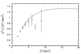
Figure 1: The Pauli form factor of the proton scaled by $Q^{6}$. Data are taken from [2]. The solid line represents the result obtained with the diquark model [7].

($\sim 1/Q^{6}$).
In explicit applications of the HSA (carried through only in leading twist and to lowest order QCD with very few exceptions) one encounters the difficulty that the data are available only at moderately large momentum transfer, a region in which non-perturbative dynamics may still play a crucial role. A general feature of such applications is the extreme sensitivity to the DAs chosen for the involved hadrons. Only strongly end-point concentrated DAs provide results which are at least for the magnetic form factor of the nucleon in fair agreement with the data [3]. This apparent success of the HSA is only achieved at the expense of strong contribution from soft regions where one of the constituents carries only a tiny fraction of its parent hadron’s momentum. This is a very problematical situation for a perturbative calculation. It should be stressed that none of the DAs used in actual applications leads to a successful description of all large momentum transfer processes investigated so far.
It seems clear from the above remarks that the HSA at leading twist although likely to be the correct asymptotic picture for exclusive reactions, needs modifications at moderately large momentum transfer. In a series of papers [4]^-[10] such a modification has been proposed by us in which baryons are viewed as composed of quarks and diquarks. The latter are treated as quasi-elementary constituents which partly survive medium hard collisions. Diquarks are an effective description of correlations in the wave functions and constitute a particular model for non-perturbative effects. The diquark model may be viewed as a variant of the HSA appropriate for moderately large momentum transfer and it is designed in such a way that it evolves into the standard pure quark HSA asymptotically. In so far the standard HSA and the diquark model do not oppose each other, they are not alternatives but rather complements. The existence of diquarks is a hypothesis. However, from experimental and theoretical approaches there have been many indications suggesting the presence of diquarks. For instance, they were introduced in baryon spectroscopy, in nuclear physics, in astrophysics, in jet fragmentation and in weak interactions to explain the famous $\Delta I=1/2$ rule. Diquarks also provide a natural explanation of the equal slopes of meson and baryon Regge trajectories. For more details and for references, see [5]. It is important to note that QCD provides some attraction between two quarks in a colour $\{\bar{3}\}$ state at short distances as is to be seen from the static reduction of the one-gluon exchange term.
Even more important for our aim, diquarks have also been found to play a role in inclusive hard scattering reactions. The most obvious place to signal their presence is deep inelastic lepton-nucleon scattering. Indeed the higher twist contributions, convincingly observed [11], can be modelled as lepton-diquark elastic scattering. Baryon production in inclusive $pp$ collisions also reveals the need for diquarks scattered elastically in the hard interaction [12]. For instance, kinematical dependences or the excess of the proton yield over the antiproton yield find simple explanations in the diquark model. No other explanation of these phenomena is known as yet.
The diquark model: As in the standard HSA a helicity amplitude for the reaction $AB\rightarrow CD$ is expressed as a convolution of DAs and hard scattering amplitudes ($s$, $-t$, $-u$   $\gg m_{i}^{2}$)

$${\large M}(s,t)\,=\,\int{\rm d}x_{C}{\rm d}x_{D}{\rm d}x_{A}{\rm d}x_{B}\Phi^{*}_{C}(x_{C})\Phi^{*}_{D}(x_{D})T_{H}(x_{i},s,t)\Phi_{A}(x_{A})\Phi_{B}(x_{B})$$ (3)

where helicity labels are omitted for convenience. Implicitly it is assumed in (3) that the valence Fock states consist of only two constituents, a quark and a diquarks (antiquark) in the case of baryons (mesons). In so far the specification of the quark momentum fraction $x_{i}$ suffices; the diquark (antiquark) carries the momentum fraction $1-x_{i}$. If an external particle is point-like, e. g. a photon, the accompanying DA is to be replaced by $\delta(1-x_{i})$. Because of QCD evolution the DAs depend logarithmically on the momentum transfer. This fact is of minor importance in the limited range of momentum transfer in which data are available and is therefore ignored. As in the standard HSA contributions from higher Fock states are neglected. This is justified by the fact that that such contributions are suppressed by powers of $\alpha_{s}/t$ as compared to those from the valence Fock state.
In the diquark model spin $0$ ($S$) and spin $1$ ($V$) colour antitriplet diquarks are considered. Within flavour SU(3) the $S$ diquarks form an antitriplet, the $V$ diquarks an sixtet. Assuming zero relative orbital angular momentum between quark and diquark and taking advantage of the collinear approximation, the valence Fock state of an ground state octet baryon $B$ with helicity $\lambda$ and momentum $p$ can be written in a covariant fashion (omitting colour indices)

$$|B;p,\lambda\rangle=f_{S}\,\Phi_{S}^{B}(x)\,B_{S}\,u(p,\lambda)+f_{V}\,\Phi_{V}^{B}(x)\,B_{V}(\gamma^{\alpha}+p^{\alpha}/m_{B})\gamma_{5}\,u(p,\lambda)/\sqrt{3}$$ (4)

where $u$ is the baryon’s spinor. The two terms in (4) represent configurations consisting of a quark and either a scalar or a vector diquark, respectively. The couplings of the diquarks with the quarks in a baryon lead to flavour functions which e. g. for the proton read

$$B_{S}=u\,S_{[u,d]}\hskip 56.9055ptB_{V}=[uV_{\{u,d\}}-\sqrt{2}d\,V_{\{u,u\}}]/\sqrt{3}\,.$$ (5)

The DAs $\Phi^{B}_{S(V)}$ are conventionally normalized as $\int{\rm d}x\Phi=1$. The constants $f_{S(V)}$ play the role the configuration space wave function at the origin.
The DAs containing the complicated non-perturbative bound state physics, cannot reliably be calculated from QCD at present. It is still necessary to parameterize the DAs and to fit the eventual free parameters to experimental data. Hence, both the models, the standard HSA as well as the diquark model, only get a predictive power when a number of reactions involving the same hadrons are investigated. In the diquark model the following DAs have been proven to work satisfactorily well in many applications [7]^-[10]:

$$\Phi^{B}_{S}(x) = N^{B}_{S}x(1-x)^{3}\exp{\left[-b^{2}(m^{2}_{q}/x+m^{2}_{S}/(1-x))\right]}$$ (6)

$$\Phi^{B}_{V}(x) = N^{B}_{V}x(1-x)^{3}(1+5.8\,x-12.5\,x^{2})\exp{\left[-b^{2}(m^{2}_{q}/x+m^{2}_{V}/(1-x))\right]}.$$

These DAs are a suitable adaption of a meson DA obtained by transforming the harmonic oscillator wave function to the light-cone. The constants $N^{B}$ are fixed through the normalization convention (e. g. for the proton $N_{S}^{p}=25.97$ and $N_{V}^{p}=22.92$). The DAs exhibit a mild flavour dependence via the exponential which also guarantees a strong suppression of the end-point regions. The masses in (6) are constituent masses since they enter through a rest frame wave function. For $u$ and $d$ quarks we take $350\,{\rm MeV}$ and for the diquarks $580\,{\rm MeV}$. Strange quarks and diquarks are assumed to be $150\,{\rm MeV}$ heavier that the non-strange ones. It is to be stressed that the quark and diquark masses only appear in the DAs (6); in the hard scattering kinematics they are neglected. The final results (form factors, amplitudes) depend on the actual mass values mildly. The transverse size parameter $b$ is fixed from the assumption of a Gaussian transverse momentum dependence of the full wave function and the requirement of a value of $600\,{\rm MeV}$ for the mean transverse momentum (actually $b=0.498\,{\rm GeV}^{-1}$). As the constituent masses the transverse size parameter is not considered as a free parameter since the final results only depend on it weakly.
The hard scattering amplitudes $T_{H}$ determined by short-distance physics, are calculated from a set of Feyman graphs relevant to a given process. Diquark-gluon and diquark-photon vertices appear in these graphs which, following standard prescriptions, are defined as

$$\mbox{SgS}: i\,g_{s}t^{a}\,(p_{1}+p_{2})_{\mu}$$

$$\mbox{VgV}: -i\,g_{s}t^{a}\,\Big{\{}g_{\alpha\beta}(p_{1}+p_{2})_{\mu}-g_{\beta\mu}\left[(1+\kappa)\,p_{2}-\kappa\,p_{1}\right]_{\alpha}$$ (7)

$$-g_{\mu\alpha}\left[(1+\kappa)\,p_{1}-\kappa\,p_{2}\right]_{\beta}\Big{\}}$$

where $g_{s}=\sqrt{4\pi\alpha_{s}}$ is the QCD coupling constant. $\kappa$ is the anomalous magnetic moment of the vector diquark and $t^{a}=\lambda^{a}/2$ the Gell-Mann colour matrix. For the coupling of photons to diquarks one has to replace $g_{s}t^{a}$ by $-\sqrt{4\pi\alpha}e_{D}$ where $\alpha$ is the fine structure constant and $e_{D}$ is the electrical charge of the diquark in units of the elementary charge. The couplings $DgD$ are supplemented by appropriate contact terms required by gauge invariance.
The composite nature of the diquarks is taken into account by phenomenological vertex functions. Advice for the parameterization of the 3-point functions (diquark form factors) is obtained from the requirement that asymptotically the diquark model evolves into the standard HSA. Interpolating smoothly between the required asymptotic behaviour and the conventional value of 1 at $Q^{2}=0$, the diquark form factors are actually parametrized as

$$\vspace*{-0.5cm}F_{S}^{(3)}(Q^{2})=\frac{Q_{S}^{2}}{Q_{S}^{2}+Q^{2}}\,,\qquad F_{V}^{(3)}(Q^{2})=\left(\frac{Q_{V}^{2}}{Q_{V}^{2}+Q^{2}}\right)^{2}\,.$$ (8)

The asymptotic behaviour of the diquark form factors and the connection to the hard scattering model is discussed in more detail in Ref. [5, 6]. In accordance with the required asymptotic behaviour the $n$-point functions for $n\geq 4$ are parametrized as

$$\vspace*{-0.8cm}F_{S}^{(n)}(Q^{2})=a_{S}F_{S}^{(3)}(Q^{2})\,,\qquad F_{V}^{(n)}(Q^{2})=\left(a_{V}\frac{Q_{V}^{2}}{Q_{V}^{2}+Q^{2}}\right)^{n-3}F_{V}^{(3)}(Q^{2}).$$ (9)

The constants $a_{S,V}$ are strength parameters. Indeed, since the diquarks in intermediate states are rather far off-shell one has to consider the possibility of diquark excitation and break-up. Both these possibilities would likely lead to inelastic reactions. Therefore, we have not to consider these possibilities explicitly in our approach but excitation and break-up lead to a certain amount of absorption which is taken into account by the strength parameters. Admittedly, that recipe is a rather crude approximation for $n\geq 4$. Since in most cases the contributions from the n-point functions for $n\geq 4$ only provide small corrections to the final results that recipe is sufficiently accurate.
Special features of the diquark model: The diquark hypothesis has striking consequences. It reduces the effective number of constituents inside baryons and, hence, alters the power laws (1). In elastic baryon-baryon scattering, for instance, the usual power $s^{-10}$ becomes $s^{-6}F(s)$ where $F$ represents the effect of diquark form factors. Asymptotically $F$ provides the missing four powers of $s$. In the kinematical region in which the diquark model can be applied ($-t$, $-u\geq 4\,{\rm GeV}^{2}$), the diquark form factors are already active, i. e. they supply a substantial $s$ dependence and, hence, the effective power of $s$ lies somewhere between 6 and 10. The hadronic helicity is not conserved in the diquark model at finite momentum transfer since vector diquarks can flip their helicities when interacting with gluons. Thus, in contrast to the standard HSA spin-flip dependent quantities like the Pauli form factor of the nucleon can be calculated.
Electromagnetic nucleon form factors: This is the simplest application of the diquark model and the most obvious place to fix the various parameters of the model. The Dirac and Pauli form factors of the nucleon are evaluated from the convolution formula (3) with the DAs (6) and the parameters are determined from a best fit to the data in the space-like region. The following set of parameters

$$\begin{array}[]{cccc}f_{S}=73.85\,\mbox{MeV},&Q_{S}^{2}=3.22\,\mbox{GeV}^{2},&a_{S}=0.15,&\\ f_{V}=127.7\,\mbox{MeV},&Q^{2}_{V}=1.50\,\mbox{GeV}^{2},&a_{V}=0.05,&\kappa=1.39\,;\end{array}$$ (10)

provides a good fit of the data [7]. $\alpha_{s}$ is evaluated with $\Lambda_{QCD}=200\,{\rm MeV}$ and restricted to be smaller than $0.5$. The parameters $Q_{S}$ and $Q_{V}$, controlling the size of the diquarks, are in agreement with the higher-twist effects observed in the structure functions of deep inelastic lepton-hadron scattering [11] if these effects are modelled as lepton-diquark elastic scattering. The Dirac form factor of the proton is perfectly reproduced. The results for the Pauli form factor are shown in Fig. 1. The predictions for the two neutron form factors are also in agreement with the data. However, more accurate neutron data are needed in the $Q^{2}$ region of interest in order to examine the model crucially. The nucleon’s axial form factor [7] and its electromagnetic form factors in the time-like regions [8] have also been evaluated. Both the results compare well with data. Even electroexcitation of nucleon resonances has been investigated [13, 14].
Real Compton scattering (RCS): $\gamma p\rightarrow\gamma p$ is the next reaction to which the diquark model is applied. Since again the only hadrons involved are protons RCS can be predicted in the diquark model; there is no free parameter to be adjusted. Typical Feynman graphs contributing to that process are shown in Fig. 2.

Figure 2: Typical Feynman graphs contributing to $\gamma^{(\ast)}\,p\rightarrow\gamma\,p$.

The results of the diquark model for RCS are shown in Fig. 3 for three different photon energies [6, 9].

Figure 3: The cross section for RCS off protons scaled by $s^{6}$ vs. $\cos\theta$ for three different photon energies. The experimental data are taken from [15].

Note that in the very forward and backward regions the transverse momentum of the outgoing photon is small and, hence, the diquark model which is based on perturbative QCD, is not applicable. Despite the rather small energies at which data [15] are available, the diquark model is seen to work rather well. The predicted cross section does not strictly scale with $s^{-6}$. The results obtained within the standard HSA are of similar quality [16]. The diquark model also predicts interesting photon asymmetries and spin correlation parameters (see the discussion in [6]). Even a polarization of the proton, of the order of $10\%$, is predicted [6]. This comes about as a consequence of helicity flips generated by vector diquarks and of perturbative phases produced by propagator poles appearing within the domains of momentum fraction integrations. The poles are handled in the usual way by the $\imath\varepsilon$ presription. The appearance of imaginary parts to leading order of $\alpha_{s}$ is a non-trivial prediction of perturbative QCD [17]; it is characteristic of the HSA and is not a consequence of the diquark hypothesis.
Two-photon annihilation into $p\bar{p}$ pairs: This process is related to RCS by crossing, i. e. the same set of Feynman graphs contributes (see Fig. 2). The only difference is that now the diquark form factors are needed in the time-like region. The expressions (8,9) represent an effective parameterization of them valid at large space-like $Q^{2}$. Since the exact dynamics of the diquark system is not known it is not possible to continue these parameterizations to the time-like region in a unique way. A continuation can be defined as follows [8]: $Q^{2}$ is replaced by $-s$ in (8,9) guaranteeing the correct asymptotic behaviour and, in order to avoid the appearance of unphysical poles at low $Q^{2}$, the diquark form factors are kept constant once their absolute values have reached $c_{0}=1.3$ [8]. The same definition of the time-like diquark form factors is used in the analysis the proton form factor in the time-like region. The diquark model predictions for the integrated $\gamma\gamma\rightarrow p\bar{p}$ cross section is compared to the CLEO data [18] in Fig. 4. At large energies the agreement

Figure 4: The integrated $\gamma\gamma\rightarrow p\bar{p}$ cross section ($\mid\cos{\theta}\mid\geq 0.6$). The solid line represents the diquark model prediction [8]. Data are taken from CLEO [18].

between predictions and experiment is good. The predictions for the angular distributions are in agreement with the CLEO data too. The standard HSA on the other hand predicts a cross section which lies about an order of magnitude below the data [19]. Recently CLEO has also measured two-photon annihilations into $\Lambda\bar{\Lambda}$ pairs [20]. Surprisingly the integrated cross section is, within errors, as large as that for annihilations into $p\bar{p}$ pairs. Using the SU(6)-like spin-flavour dependence (4,6), the diquark model predicts a $\Lambda\bar{\Lambda}$ cross section which is about a factor of 2 smaller than the CLEO data. The reason for this discrepancy is not yet understood.
Virtual Compton scattering (VCS): This process is accessible through $ep\rightarrow ep\gamma$. An interesting element in that reaction is that, besides VCS, there is also a contribution from the Bethe-Heitler (BH) process where the final state photon is emitted from the electron. Electroproduction of photons offers many possibilities to test details of the dynamics: One may measure the $s$, $t$ and $Q^{2}$ dependence as well as that on the angle $\phi$ between the hadronic and leptonic scattering planes. This allows to isolate cross sections for longitudinal and transverse virtual photons. One may also use polarized beams and targets and last but not least one may measure the interference between the BH and the VC contributions. The interference is sensitive to phase differences.
At $s$, $-t$ and $-u\gg m_{p}^{2}$ (or small $|\cos{\theta}|$ where $\theta$ is the scattering angle of the outgoing photon in the photon-proton center of mass frame) the diquark model can also be applied to VCS [9]. Again there is no free parameter in that calculation. The relevant Feynman graphs are the same as for RCS (see Fig. 2). The model can safely be applied for $s\geq 10\,{\rm GeV}^{2}$ and $|\cos{\theta}|\leq 0.6$. For the future CEBAF beam energy of $6\,{\rm GeV}$ the model is at its limits of applicability. However, since the diquark model predictions for real Compton scattering do rather well agree with the data even at $s\geq 5\,{\rm GeV}^{2}$ (see Fig. 3) one may expect similarly good agreement for VCS. Predictions for the VCS cross section are shown in Fig. 5. The transverse

Figure 5: The cross section for VCS vs. $\cos\theta$ for several values of $Q^{2}/s$ at $s=5\;{\rm GeV}^{2}$. Upper left: the transverse cross section scaled by $s^{6}$. Upper right: the ratio of the longitudinal over the transverse cross sections. Lower left (right): the ratio of the longitudinal (transverse) - transverse interference term over the transverse cross section.

cross section (which, at $Q^{2}=0$, is the cross section for RCS is the dominant piece. The other cross sections only become sizeable for large values of $|\cos{\theta}|$. Examination of the Bethe-Heitler contribution to the process $ep\to ep\gamma$ reveals that it is small as compared to the VCS contribution at high energies, small values of $|\cos{\theta}|$ and for an out-of-plane experiment, i. e. $\phi\geq 50^{\circ}$.
The last observable I want to discuss is the electron asymmetry in $ep\to ep\gamma$:

$$A_{L}\,=\,\frac{\sigma(+)-\sigma(-)}{\sigma(+)+\sigma(+)}$$ (11)

where $\pm$ indicates the helicity of the incoming electron. $A_{L}$ measures the imaginary part of the longitudinal – transverse interference. The longitudinal amplitudes for VCS turn out to be small in the diquark model (hence $A_{L}^{VC}$ is small). However, according to the model, $A_{L}$ is large in the region of strong BH contamination (see Fig. 6). In that region, $A_{L}$ measures the relative phase

Figure 6: The electron asymmetry in $ep\to ep\gamma$ as predicted by the diquark model [9].

(being of perturbative origin from on-shell going internal gluons, quarks and diquarks [17]) between the BH amplitudes and the VCS ones. The magnitude of the effect shown in Fig. 6 is sensitive to details of the model and, therefore, should not be taken literally. Despite of this our results may be taken as an example of what may happen. The measurement of $A_{L}$, e. g. at CEBAF, will elucidate strikingly the underlying dynamics of VCS.
Photo- and electroproduction of mesons: This is already a quite complicated reaction to which all together 158 Feynman graphs contribute. Up to now only the two processes $\gamma p\rightarrow K^{+}\Lambda$, $K^{*+}\Lambda$ have been investigated [10]. The analyses of other final states as well as electroproduction are in progress. The calculation of $K\Lambda$ production is somewhat simpler than that for other final states because only scalar diquarks contribute. The analysis of many different final states will provide deep insight in the dynamics.
As compared to the processes discussed above a new element appears now, namely the mesonic DA. Comparison of predictions with data [21] (see Fig. 7) revealed that the asymptotic form of the Kaon DA ($\sim x(1-x)$) works very well (using the standard value of

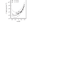
Figure 7: Differential cross section for $\gamma p\rightarrow K^{+}\Lambda$ scaled by $s^{7}$ vs. $\cos{\theta_{cm}}$. Solid (dash-double-dotted) line: Diquark model result [10] at $p^{\gamma}_{lab}=6(4)\,{\rm GeV}$ using the asymptotic Kaon DA. Short-dashed line: Results $p^{\gamma}_{lab}=6\,{\rm GeV}$ using the CZ Kaon DA. Long-dashed line: Predictions from the standard HSA [22]. The data are taken from Anderson et al. [21].

the Kaon decay constant). On the other hand the double-humped DA proposed by Chernyak and Zhitnitski [3] fails, the predicted cross section is too large as compared with the data. The predictions from the standard HSA [22] are smaller than those from the diquark model. It should be mentioned that for the $\Lambda$ the SU(6)-like spin-flavour dependence (4, 6) is used. How to reconcile this with the apparent failure of the SU(6)-like $\Lambda$ wave function in $\gamma\gamma\to\Lambda\bar{\Lambda}$ remains to be seen.
Summary and outlook: The diquark model which represents a variant of the HSA, combines perturbative QCD with non-perturbative elements. The diquarks represent quark-quark correlations in baryon wave functions which are modelled as quasi-elementary constituents. This model has been applied to many photon induced exclusive processes at moderarely large momentum transfer (typically $\geq 4\,{\rm GeV}^{2}$). From the analysis of the nucleon form factors the parameters specifying the diquark and the DAs, are fixed. Compton scattering and two-photon annihilations of $p\bar{p}$ can then be predicted. The comparison with existing data reveals that the diquark model works quite well and in fact much better then the pure quark HSA. Using the asymptotic DA for the Kaon and SU(6) ideas to fix the $\Lambda$ DA one can also predict photoproduction of $K\Lambda$. Again there is agreement between predictions and experiment.
Predictions for the VCS cross section and for the $ep\to ep\gamma$ cross section have also been made for kinematical situations accessible at the upgraded CEBAF and perhaps at future high energy accelerators like ELFE@HERA. According to the diquark model the BH contamination of the photon electroproduction becomes sizeable for small azimuthal angles. The BH contribution also offers the interesting possibility of measuring the relative phases between the VC and the BH amplitudes. The phases of the VC amplitudes are a non-trivial phenomenon generated by the fact that some of the internal quarks, diquarks and gluons may go on mass shell. The electron asymmetry $A_{L}$ is particularly sensitive to relative phases. In contrast to the standard HSA the diquark model allows to calculate helicity flip amplitudes, the helicity sum rule (2) does not hold at finite $Q^{2}$. One example of an observable controlled by helicity flip contributions is the Pauli form factor of the proton. Also in this case the diquark model accounts for the data.

References

References

- [1] G. P. Lepage and S. J. Brodsky, Phys. Rev. D 22, 2157 (1980).
- [2] P. Bosted et al., Phys. Rev. Lett. 68, 3841 (1992).
- [3] V. L. Chernyak and A. R. Zhitnitsky, Phys. Rep. 112, 173 (1984).
- [4] M. Anselmino, P. Kroll and B. Pire, Z. Phys. C 36, 89 (1987).
- [5] P. Kroll, Proceedings of the Adriatico Research Conference on Spin and Polarization Dynamics in Nuclear and Particle Physics, Trieste, 1988.
- [6] P. Kroll, W. Schweiger and M. Schürmann, Int. Jour. of Mod. Physics A 6, 4107 (1991)
- [7] R. Jakob, P. Kroll, M. Schürmann and W. Schweiger, Z. Phys. A 347, 109 (1993).
- [8] P. Kroll, Th. Pilsner, M. Schürmann and W. Schweiger, Phys. Lett. B 316, 546 (1993).
- [9] P. Kroll, M. Schürmann and P. Guichon, Nucl. Phys. A 598, 435 (1996).
- [10] P. Kroll, M. Schürmann, K. Passek and W. Schweiger, preprint UNIGRAZ - UTP 15-04-96.
- [11] M. Virchaux and A. Milsztajn, Phys. Lett. B 274, 221 (1992).
- [12] A. Breakstone et al., Z. Phys. C 28, 335 (1985).
- [13] P. Kroll, M. Schürmann and W. Schweiger, Z. Phys. A 342, 429 (1992).
- [14] J. Bolz, P. Kroll and J. G. Körner, Z. Phys. A 350, 145 (1994).
- [15] M. A. Shupe et al., Phys. Rev. D 19, 1921 (1979).
- [16] A. S. Kronfeld and B. , Phys. Rev. D 44, 3445 (1991).
- [17] G. R. Farrar et al., Phys. Rev. Lett. 62, 2229 (1989).
- [18] M. Artuso et al., CLEO collaboration, Phys. Rev. D 50, 5484 (1994).
- [19] G. R. Farrar, E. Maina and F. Neri, Nucl. Phys. B 259, 702 (1985); B 263, 746 (1986)(E).
- [20] D. W. Bliss, representing the CLEO collaboration, APS meeting 1996.
- [21] R. L. Anderson et al., Phys. Rev. D 14, 679 (1976).
- [22] G. R. Farrar, K. Huleihel and H. Zhang, Nucl. Phys. B 349, 655 (1991).