Chargino Pair Production at LEP2 with Broken R-Parity: 4-jet Final States

Abstract

We study the pair production of charginos in $e^{+}e^{-}$-collisions followed by the decay via R-parity violating $LQ{\bar{D}}$ operators. We determine the complete matrix element squared for chargino decays via $LQ{\bar{D}}$ or $LL{\bar{E}}$ operators. We find regions in MSSM parameter space where the chargino mass is $52.5\,GeV$ and the R-parity violating decays of the charginos dominate the gauge decays to neutralinos. At LEP2 this then leads to additional 4 jet events which could explain the excess recently observed by ALEPH.

Submitted to Physics Letters B.

1 Introduction

Supersymmetry predicts many new particles with thresholds possibly within reach of the LEP2 collider at CERN [1]. Chargino pair production is a promising candidate for a first signal. It has been widely studied [2] within the minimal supersymmetric standard model (MSSM), where R-parity $R_{p}=(-)^{2S+3B+L}$ is conserved. There the chargino cascade decays to the lightest neutralino which is stable and escapes detection. The signal is partly characterised by missing transverse momentum.

From a theoretical point of view it is just as likely that $R_{p}$ is violated (${\not\!\!R_{p}}$) [3, 4]. The lightest supersymmetric particle is then no longer stable. If it decays within the detector the missing transverse momentum signal is diluted and the signal has other main characteristics [5]. Direct searches for lepton signals in ALEPH at LEPI energies have previously addressed this issue [6], and have shown that the SUSY limits obtained from searches under the assumption of $R_{p}$ conservation also hold under the simultaneous violation of R-parity and lepton number. It is the purpose of this letter to study the production and decay of charginos at LEP2 with broken R-parity with particular emphasis on 4-jet final states.

Recently ALEPH observed anomalously large 4-jet production at LEP2 while running at $\sqrt{s}=133-136\,GeV$ [7]. There have been several proposed solutions [8] in particular two [9, 10] which also propose mechanisms within supersymmetry with broken R-parity. Of the latter two, the first considers pair production of scalar sneutrinos and their subsequent decay via an $LQ{\bar{D}}$ operator. The second considers squark pair production followed by the decay via a ${\bar{U}}{\bar{D}}{\bar{D}}$ operator. We present here a third possible explanation via broken R-parity namely the production and decay of charginos. As we see below, this is experimentally distinguishable and relies on the $LQ{\bar{D}}$ operator.

When R-parity is broken the superpotential contains the additional baryon- and lepton-number violating Yukawa couplings [11]

$$W_{{\not\!R_{p}}}=\lambda_{ijk}L_{i}L_{j}{\bar{E}}_{k}+\lambda^{\prime}_{ijk}L_{i}Q_{j}{\bar{D}}_{k}+\lambda^{\prime\prime}_{ijk}{\bar{U}}_{i}{\bar{D}}_{j}{\bar{D}}_{k}.$$ (1)

The superpotential contains 45 operators; combinations of the lepton- and baryon-number violating couplings can lead to proton decay in disagreement with the experimental bounds [12]. Thus some symmetry must be imposed which prohibits a subset of the terms. Several examples have been considered in the literature [4]. In most models motivated by unification (including gravity), there is a preference for allowing the lepton number violating terms over the baryon number violating terms. In addition, the strictest laboratory bounds are on the lowest generation ${\bar{U}}_{i}{\bar{D}}_{j}{\bar{D}}_{k}$ operators, e.g. $\lambda^{\prime\prime}_{121}<10^{-6}$ [13] rendering them unimportant for collider searches. It is difficult to construct models which allow for large higher generation couplings $\lambda^{\prime\prime}$ and which still satisfy this strict bound on $\lambda^{\prime\prime}_{121}$ since the quark mixing is known to be non-zero. In our specific example below, we shall thus focus on the case of a single dominant $L_{i}Q_{j}{\bar{D}}_{k}$ operator. The present experimental bounds on these operators are given in Table 1. The $LQ{\bar{D}}$ operators do not affect chargino production but can significantly alter the decay patterns of the charginos. As we show below, in relevant regions of parameter space the R-parity violating decay of the chargino dominates. These decays then lead to four jet final states which could explain the discrepancy observed by ALEPH.

$\lambda^{\prime}_{111}$	0.0004	$\lambda^{\prime}_{211}$	0.09	$\lambda^{\prime}_{311}$	0.14
$\lambda^{\prime}_{112}$	0.03	$\lambda^{\prime}_{212}$	0.09	$\lambda^{\prime}_{312}$	0.14
$\lambda^{\prime}_{113}$	0.03	$\lambda^{\prime}_{213}$	0.09	$\lambda^{\prime}_{313}$	0.14
$\lambda^{\prime}_{121}$	0.26	$\lambda^{\prime}_{221}$	0.18	$\lambda^{\prime}_{321}$	-
$\lambda^{\prime}_{122}$	0.45	$\lambda^{\prime}_{222}$	0.18	$\lambda^{\prime}_{322}$	-
$\lambda^{\prime}_{123}$	0.26	$\lambda^{\prime}_{223}$	0.18	$\lambda^{\prime}_{323}$	-
$\lambda^{\prime}_{131}$	0.26	$\lambda^{\prime}_{231}$	0.44	$\lambda^{\prime}_{331}$	0.26
$\lambda^{\prime}_{132}$	0.51	$\lambda^{\prime}_{232}$	0.44	$\lambda^{\prime}_{332}$	0.26
$\lambda^{\prime}_{133}$	0.001	$\lambda^{\prime}_{233}$	0.44	$\lambda^{\prime}_{333}$	0.26

Table 1: Bounds on the Yukawa couplings of the $L_{i}Q_{j}{\bar{D}}_{k}$ operators [14]. The bounds are all to be multiplied by a scalar fermion mass ${\tilde{M}}_{0}/100\,GeV$ except for the bound on $\lambda^{\prime}_{111}$ which also depends on the gluino mass [15]. There are no bounds on the couplings $\lambda^{\prime}_{32k}$.

2 Chargino Decays

2.1 SUSY Spectrum

The decay pattern of the chargino depends foremost on the supersymmetric spectrum. In low energy supersymmetry, when $SU(2)_{L}\times U(1)_{Y}$ has been broken to $U(1)_{em}$ the gauginos mix with the Higgsinos to form the chargino and neutralino mass eigenstates. The masses depend on the $SU(2)_{L}$, $U(1)_{Y}$ gaugino masses $M_{2}$, and $M_{1}$, the Higgs mixing parameter $\mu$ and the ratio of the vacuum expectation values $\tan\beta$. For any fixed values of these parameters, we can determine the gaugino spectrum completely. In particular, we can determine the nature of the lightest supersymmetric particle (LSP), and which gaugino decay modes are kinematically accessible to the chargino.

In grand unified theories $M_{2}$ and $M_{1}$ are related by $M_{1}=\frac{5}{3}\tan^{2}\theta_{W}M_{2}$. We shall impose this constraint throughout this letter and we thus only have 3 free parameters in the gaugino sector: $(M_{2},\,\mu,\,\tan\beta)$. In Fig. 2 we have fixed $\tan\beta=2,35$. For $\tan\beta=2$ the black band denotes the range of parameters where the chargino is the LSP. In this range the chargino mass is never above $\approx 23\,GeV$. For $M_{\chi^{+}}<(M_{Z^{0}}/2)$ the chargino can contribute to the $Z^{0}$  width. This is independent of the chargino decay and therefore does not depend on whether R-parity is conserved or not. LEP1 measurements of the $Z^{0}$width have determined a model independent lower bound on the mass of the chargino of $M_{\chi^{+}}\geq 45.2\,GeV$ [18]. This is included in Fig.2 as a narrow dashed curve. We see that within the SUSY-GUT framework, given the experimental constraints, the chargino can not be the LSP. For $\tan\beta=35$ there is also a band where the chargino is the LSP but it is very small and below the resolution of Fig.2. It is excluded by the LEP1 measurement as well.

2.2 Matrix Element

We now study the ${\not\!\!R_{p}}$ chargino decays for the explicit case of a $L_{i}Q_{j}{\bar{D}}_{k}$ operator. As we discuss in the appendix, the results can be easily translated to the decay via a $L_{i}L_{j}{\bar{E}}_{k}$ operator. A positively charged chargino ${{\tilde{\chi}}^{+}}_{l}$ can decay to the following final states

$${{\tilde{\chi}}^{+}}_{l}\rightarrow\left\{\begin{array}[]{l}{\nu}_{i}+u_{j}+{\bar{d}}_{kR}\,\,\,\,\,\,\,\,(\ref{eq:finalstates}.1)\\ e_{i}^{+}+{\bar{d}}_{j}+{d}_{kR}\,\,\,\,\,\,(\ref{eq:finalstates}.2)\\ e_{i}^{+}+{\bar{u}}_{j}+{u}_{kR}\,\,\,\,\,\,(\ref{eq:finalstates}.3)\\ {\bar{\nu}}_{i}+{\bar{d}}_{j}+{u}_{kR}\,\,\,\,\,\,\,\,(\ref{eq:finalstates}.4)\end{array}\right.$$ (6)

Figure 1: Feynman diagrams for direct ${\not\!\!R_{p}}$ Chargino decays via the $L_{i}Q_{j}{\bar{D}}_{k}$ operator.

Figs.(1a)-(1f) show the Feynman diagrams for chargino decays into the final states (6.1)-(6.4). The ${\not\!\!R_{p}}$ vertices are labelled by the Yukawa coupling strength ($\lambda^{\prime}_{ijk}$). Note that there are two diagrams (1a,b) and (1c,d) for the final states (6.1) and (6.2) respectively. For the four decay modes the amplitudes squared are given by

$$|{\cal M}_{1}|^{2} = 4n_{c}g^{2}{\lambda^{\prime}}^{2}\left[\frac{\alpha_{R}^{2}}{R^{2}({\tilde{e}}_{iL})}({{\chi}^{+}_{l}}\cdot{\nu_{i}})({u_{j}}\cdot{{\bar{d}}_{k}})\right.$$ (7)

$$+\frac{({\nu_{i}}\cdot{{\bar{d}}_{k}})}{R^{2}({\tilde{d}}_{jL})}\left\{(\beta_{L}^{2}+\beta_{R}^{2})({{{\chi}^{+}_{l}}}\cdot{u_{j}})+2{\cal R}e(\beta_{L}\beta_{R}^{*}m_{uj}M_{{{\chi}^{+}_{l}}})\right\}$$

$$\left.-{\cal R}e\left\{\frac{\alpha_{R}}{R({\tilde{e}}_{iL})R({\tilde{d}}_{jL})}\left(\beta_{L}^{*}m_{uj}M_{{{\chi}^{+}_{l}}}({u_{j}}\cdot{{\bar{d}}_{k}})+\beta_{R}^{*}{\cal G}(p,\nu_{i},{\bar{d}}_{k},u_{j})\right)\right\}\right]$$

$$|{\cal M}_{2}|^{2} = 4n_{c}g^{2}{\lambda^{\prime}}^{2}\left[\frac{({d_{j}}\cdot{{\bar{d}}_{k}})}{R^{2}({\tilde{\nu}}_{iL})}\left\{(\gamma_{L}^{2}+\gamma_{R}^{2})({{{\chi}^{+}_{l}}}\cdot{e_{i}})+2{\cal R}e(\gamma_{L}\gamma_{R}^{*}m_{ei}M_{{{\chi}^{+}_{l}}})\right\}\right.$$ (8)

$$+\frac{({e_{i}}\cdot{{\bar{d}}_{k}})}{R^{2}({\tilde{u}}_{jL})}\left\{(\delta_{L}^{2}+\delta_{R}^{2})({{{\chi}^{+}_{l}}}\cdot{d_{j}})+2{\cal R}e(\delta_{L}\delta_{R}^{*}m_{dj}M_{{{\chi}^{+}_{l}}})\right\}$$

$$\left.-\frac{1}{R({\tilde{\nu}}_{iL})R({\tilde{u}}_{jL})}{\cal R}e\left\{\gamma_{L}\delta_{L}^{*}{\cal G}({{\chi}^{+}_{l}},e_{i},{\bar{d}}_{k},d_{j})+\gamma_{L}\delta_{R}^{*}m_{dj}M_{{{\chi}^{+}_{l}}}({e_{i}}\cdot{{\bar{d}}_{k}})\right.\right.$$

$$\left.\left.+\gamma_{R}\delta_{L}^{*}m_{ei}M_{{{\chi}^{+}_{l}}}({d_{j}}\cdot{{\bar{d}}_{k}})+\gamma_{R}\delta_{R}^{*}m_{ei}m_{dj}({{{\chi}^{+}_{l}}}\cdot{{\bar{d}}_{k}})\right\}\right]$$

$$|{\cal M}_{3}|^{2} = \frac{2n_{c}{\lambda^{\prime}}^{2}g^{2}m_{dk}^{2}|U_{l2}|^{2}}{M_{W}^{2}\cos^{2}\beta R^{2}({\tilde{d}}_{kR})}({e_{i}}\cdot{u_{j}})({{{\chi}^{+}_{l}}}\cdot{u_{k}})$$ (9)

$$|{\cal M}_{4}|^{2} = \frac{2n_{c}{\lambda^{\prime}}^{2}g^{2}m_{dk}^{2}|U_{l2}|^{2}}{M_{W}^{2}\cos^{2}\beta R^{2}({\tilde{d}}_{kR})}({\nu_{i}}\cdot{d_{j}})({{{\chi}^{+}_{l}}}\cdot{u_{k}})$$ (10)

$\alpha_{L,R},\beta_{L,R},\gamma_{L,R}$ and $\delta_{L,R}$ are couplings and are given in the appendix. The final-state momenta are denoted by the particle symbols. $M_{{{\chi}^{+}_{l}}}$ is the chargino mass and $m_{ei,dj,dk}$ are the final state fermion masses. $n_{c}=3$ is the colour factor. The function ${\cal G}(a,b,c,d)=({a}\cdot{b})({c}\cdot{d})-({a}\cdot{c})({b}\cdot{d})+({a}\cdot{d})({b}\cdot{c})$. The square of the propagators $R(p)$ are given in the appendix. We have included all mass effects. In most applications $\beta_{L},\gamma_{R},\delta_{R}\approx 0$. For $j=3$, $\beta_{L}$ is not negligible but the decay $\chi^{+}\rightarrow\nu_{i}+t+{\bar{d}}_{kR}$ is kinematically prohibited unless $M_{\chi^{+}}>m_{top}$. For large $\tan\beta$ and $i,j=3$ $\gamma_{R},\delta_{R}$ can be important. Note that the last two decay modes are proportional to $(m_{dkR}/(\cos\beta M_{W}))^{2}$ and are thus suppressed in most of the parameter space. The analogous decay of the neutralino has been given in [19]. The partial widths are given by the integration over phase space

$$\Gamma_{l}=\int\frac{1}{2\pi^{3}}\frac{1}{16M_{{\chi}^{+}_{l}}}|{\cal M}_{l}|^{2}dE_{i}dE_{j}$$ (11)

and we have averaged over the initial spin states of the chargino. If we neglect the final state masses the integrals can be performed analytically. We find

$$\Gamma_{1}({{\tilde{\chi}}^{+}}_{l}\rightarrow{\nu}_{i}+u_{j}+{\bar{d}}_{k})=4n_{c}g^{2}{\lambda^{\prime}}^{2}\left[\alpha_{R}^{2}A(\mu_{\tilde{e}_{iL}})+(\beta_{L}^{2}+\beta_{R}^{2})A(\mu_{\tilde{d}_{jL}})+{\cal R}e(\alpha_{R}\beta_{R}^{*})B(\mu_{\tilde{e}_{iL}},\mu_{\tilde{d}_{jL}})\right]$$ (12)

In the above equation,

$$A(\mu_{\tilde{e}_{iL}})=\frac{1}{32}\left[-5+6\mu_{\tilde{e}_{iL}}^{2}+(2-8\mu_{\tilde{e}_{iL}}^{2}+6\mu_{\tilde{e}_{iL}}^{4})\ln\left(\frac{\mu_{\tilde{e}_{iL}}^{2}-1}{\mu_{\tilde{e}_{iL}}^{2}}\right)\right]$$ (13)

where

$$\mu_{\tilde{e}_{iL}}=\frac{m_{\tilde{e}_{i}}}{M_{\tilde{\chi}}^{+}}$$ (14)

are the dimensionless normalized masses. $B(\mu_{\tilde{e}_{iL}},\mu_{\tilde{d}_{jL}})$ arises from the interference term and can be expressed as

$$B(\mu_{\tilde{e}_{iL}},\mu_{\tilde{d}_{jL}})=\frac{1}{4}I(\mu_{\tilde{e}_{iL}},\mu_{\tilde{d}_{jL}})+\frac{1}{32}C(\mu_{\tilde{e}_{iL}},\mu_{\tilde{d}_{jL}})$$ (15)

where

$$I=\int_{0}^{1/2}(x-2x^{2}+x\mu_{\tilde{d}_{jL}}^{2}-\mu_{\tilde{d}_{jL}}^{4})\ln(\mu_{\tilde{d}_{jL}}^{2}-2x)/(-1+2x+\mu_{\tilde{e}_{iL}}^{2})dx$$ (16)

and

$$C(\mu_{\tilde{e}_{iL}},\mu_{\tilde{d}_{jL}}) = -4\mu_{\tilde{d}_{jL}}^{2}+(1-2\mu_{\tilde{d}_{jL}}^{2}-2\mu_{\tilde{e}_{iL}}^{2})\ln(\mu_{\tilde{d}_{jL}}^{2})+4(\mu_{\tilde{d}_{jL}}^{2}-\mu_{\tilde{d}_{jL}}^{2}\mu_{\tilde{e}_{iL}}^{2})\psi$$ (17)

$$+2(\mu_{\tilde{d}_{jL}}^{2}-2\mu_{\tilde{d}_{jL}}^{4}+\mu_{\tilde{e}_{iL}}^{2}-\mu_{\tilde{d}_{jL}}^{2}\mu_{\tilde{e}_{iL}}^{2}-\mu_{\tilde{e}_{iL}}^{4})\ln(\mu_{\tilde{d}_{jL}}^{2})\psi$$

Note that in the above, all terms in $A,B$ are normalised with respect to the chargino mass $M_{\tilde{\chi}}^{+}$. $\psi=\ln\{(\mu_{\tilde{e}_{iL}}^{2}-1)/\mu_{\tilde{e}_{iL}}^{2}\}$. For $\Gamma_{2}$ we find an identical expression, with the only change being in the masses of the propagators, as one can see from the Feynman diagrams of Figure 1. When the final state masses are neglected $\Gamma_{3}=\Gamma_{4}=0$.

2.3 Chargino Width and Lifetime

If we only consider one non-zero operator $L_{i}Q_{j}{\bar{D}}_{k}$ the ${\not\!\!R_{p}}$ decay width is given by

$$\Gamma_{\not\!R_{p}}=\Gamma_{1}+\Gamma_{2}+\Gamma_{3}+\Gamma_{4}.$$ (18)

In the MSSM there are possible further ($R_{p}$-conserving) cascade decays of the chargino ${\tilde{\chi}}^{+}_{l}$ via a virtual W-boson to a lighter neutralino ${\tilde{\chi}}^{0}_{m}$

$${\tilde{\chi}}^{+}_{l} \rightarrow l^{+}+\nu+{\tilde{\chi}}^{0}_{m},$$ (19)

$${\tilde{\chi}}^{+}_{l} \rightarrow q+{\bar{q}}^{\prime}+{\tilde{\chi}}^{0}_{m}.$$ (20)

We denote the MSSM contributions to the chargino width as $\Gamma_{MSSM}$. The MSSM decay rates have been calculated by various authors [20] and they are functions of the three free parameters ($M_{2},\mu,\tan\beta$). The total chargino width is given by

$$\Gamma_{{\tilde{\chi}}^{+}}=\Gamma_{\not\!R_{p}}+\Gamma_{MSSM}.$$ (21)

Eventhough the chargino is not the LSP it will nevertheless dominantly decay directly to an R-parity even final state via the decays (6.1)-(6.4) if the ratio $\frac{\Gamma_{\not\!R_{p}}}{\Gamma_{MSSM}}$ is sufficiently large. This happens in regions of the MSSM parameter space in which the MSSM cascade decays of the chargino (19)-(20) are phase space supressed, i.e. when $M_{{\tilde{\chi}}^{+}}\approx M_{{\tilde{\chi}}^{0}}$, and when the Yukawa coupling $\lambda^{\prime}_{ijk}$ is not too small. In order to explore the ratio $\frac{\Gamma_{\not\!R_{p}}}{\Gamma_{MSSM}}$ numerically we consider a fixed SUSY scalar mass spectrum: $m_{{\tilde{q}}}=500\,GeV$, ${m_{{\tilde{l}}_{L}}}=200\,GeV$, ${m_{{\tilde{l}}_{R}}}=m_{\tilde{\nu}}=100\,GeV$. The ratio ${m_{{\tilde{l}}_{L}}}/m_{\tilde{\nu}}\geq 2$ was chosen to optimize our 4-jet signal. It is consistent with supergravity (SUGRA) models which generally predict squarks to be the heaviest and sneutrinos and right-handed sleptons to be the lightest SUSY scalar particles, but is not a generic feature, i.e. there are regions in SUGRA parameter space where the ratio is only slightly greater than 1 [21]. A factor of $\sim 1.7$ is sufficient for our argument.

                 

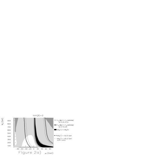
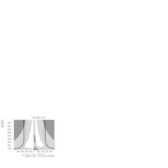
Figure 2: Regions in the $M_{2}-\mu$ parameter space in which $\Gamma_{\not\!\!R_{p}}>\Gamma_{MSSM}$ at $\lambda^{\prime}_{ijk}=0.3$ (light grey area) and $\lambda^{\prime}_{ijk}=0.03$ (dark grey area), and in which the chargino is the LSP (black region) for a) $\tan\beta=2$ and b) $\tan\beta=35$. Superimposed are contours of $M_{{\tilde{\chi}}^{+}}=52.5\,GeV$, the region where ALEPH sees an excess in 4-jet events.

In Figs.2a,b we plot regions in the $M_{2}-\mu$ gaugino parameter space in which $\Gamma_{\not\!R_{p}}>\Gamma_{MSSM}$ for a coupling strength of $\lambda^{\prime}_{ijk}=0.3$ (light grey area) and $\lambda^{\prime}_{ijk}=0.03$ (dark grey area). As mentioned above, the black area indicates the chargino LSP region in which the chargino always decays $R_{p}$-violating. For the large Yukawa coupling of $\lambda^{\prime}_{ijk}=e=0.3$ the direct ${\not\!\!R_{p}}$ chargino decays dominate over the MSSM cascade decays throughout nearly the entire $M_{2}-\mu$ plane. This is because the MSSM decay to the neutralino is phase space suppressed whereas the ${\not\!\!R_{p}}$ decay is not coupling suppressed. However, even for $\lambda=0.03$ there is still a substantial region of parameter space at large $M_{2}$ where $\Gamma_{\not\!R_{p}}$ dominates. Here $M_{\chi^{+}_{1}}\approx M_{\chi^{0}_{1}}$ and the $\chi^{+}\chi^{0}W^{+}$ coupling is small. We discuss the phenomenological consequences in more detail in section 3.2.

Figure 3: Width/Lifetime of the Chargino.

We now turn to the chargino lifetime. Fig.3 shows the chargino width and lifetime as a function of $\mu$ for one particular value of $M_{2}=700\,GeV$ and $\tan\beta=35$. The solid line shows the total width $\Gamma_{{\tilde{\chi}}^{+}}=\Gamma_{\not\!R_{p}}+\Gamma_{MSSM}$ at $\lambda^{\prime}_{ijk}=0.3$, while the broken line shows the ${\not\!\!R_{p}}$ contribution alone. The latter scales with $\lambda^{\prime 2}_{ijk}$ as seen in Eqs.(7-10). So it is clear that the chargino always decays within the detector. This also holds for smaller values of $M_{2}$ and $\tan\beta$.

2.4 Branching Fractions

We now determine the branching ratios of the chargino decays into the final states (6.1)-(6.4). The decays (6.3) and (6.4) are supressed with respect to (6.1) and (6.2) by $({\frac{m_{dk}}{\sqrt{2}M_{W}\cos\beta}})^{2}$ because the exchanged virtual right-handed down-type squark ${\tilde{\bar{d}_{R}}}$ (see also diagrams 1e and 1f) only couples Higgsino-like to the chargino. The decays (6.1) and (6.2) are comparable if the scalar fermion masses are, i.e. $m_{{\tilde{\nu}}}\approx m_{{\tilde{e}}}\approx m_{{\tilde{u}}}\approx m_{{\tilde{d}}}$. However as pointed out earlier, the four-jet signal discussed below is enhanced for $m_{{\tilde{\nu}}}<m_{{\tilde{e}}L}$. The ratios of the decay widths are given by

$${\Gamma}_{1}:{\Gamma}_{2}:{\Gamma}_{3}:{\Gamma}_{4}=({\frac{{m_{\tilde{\nu}}}}{{m_{{\tilde{e}}_{L}}}}})^{4}:1:({\frac{7\times 10^{-6}}{\cos^{2}\beta}})({\frac{{m_{{\tilde{\nu}}}}}{{{m_{{\tilde{d}}_{R}}}}}})^{4}:({\frac{7\times 10^{-6}}{\cos^{2}\beta}})({\frac{{m_{{\tilde{\nu}}}}}{{{m_{{\tilde{d}}_{R}}}}}})^{4}.$$ (22)

For our specific model, in which we fix $m_{{\tilde{q}}}=500\,GeV$, $m_{{\tilde{l}}_{L}}=200\,GeV$, $m_{{\tilde{l}}_{R}}=m_{\tilde{\nu}}=100\,GeV$, and $\tan\beta=35$,

$${\Gamma}_{1}:{\Gamma}_{2}:{\Gamma}_{3}:{\Gamma}_{4}=6\times 10^{-2}:1:10^{-5}:10^{-5}$$ (23)

the decay mode (6.2) is dominant over the entire $M_{2}-\mu$ plane. Thus from now on we neglect the other decay modes and restrict ourselves to the decay $\chi^{+}\rightarrow e_{i}^{+}+{\bar{d}}_{j}+d_{Rk}$. This essential conclusion holds for $m_{{\tilde{e}}_{L}}/m_{{\tilde{\nu}}}\stackrel{{\scriptstyle>}}{{\sim}}1.7$.

2.5 Decay Distributions

We consider the energy distributions of the chargino decay products for the decay ${\tilde{\chi}}^{+}\rightarrow e_{i}^{+}+d_{j}+{\bar{d}}_{k}$. The most sizeable effect on the charged lepton momentum is excerted by the ${\tilde{\nu}}$-propagator (Fig.1c). For $m_{\tilde{\nu}}\approx M_{{\tilde{\chi}}^{+}}$ the energy spectrum of the charged lepton, $E_{e_{i}}$, is soft. The quark energy spectra $E_{d_{j},{\bar{d}}_{k}}$ are much harder. This effect is demonstrated in Fig.4a. The $E_{e_{i}}$ spectrum becomes harder the greater the mass difference $m_{\tilde{\nu}}-M_{\chi^{+}}$. However, even for $m_{\tilde{\nu}}=100\,GeV$ it is still substantially softer than the quark spectrum.

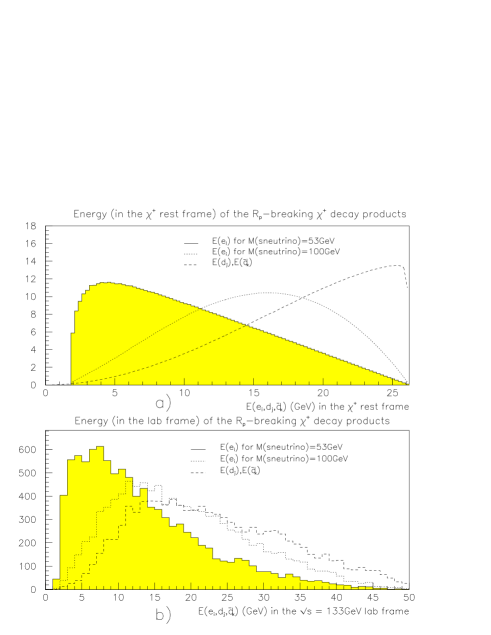
Figure 4: Energy distribution of the ${\tilde{\chi}}^{+}$ decay products. Here $\mu=54.5\,GeV$, $M_{2}=500\,GeV$, and $M_{{\tilde{\chi}}+}=52.5\,GeV$. Plot a) shows the Energy in the ${\tilde{\chi}}^{+}$ rest frame, plot b) shows the Energy in the LEP lab frame.

3 Chargino Production and Signals

We now turn to the ${\not\!\!R_{p}}$ chargino signals at LEP. First we briefly mention the more conventional ${\not\!\!R_{p}}$ signal from chargino production, before we focus on the most interesting signal, the direct ${\not\!\!R_{p}}$ chargino decays which could explain the recently observed excess in 4-jets by the ALEPH collaboration [7] with a combined invariant mass of $\sum M\approx 105\,GeV$.

3.1 Chargino Cascade Decays and Neutralino LSP Models

For a ${\not\!\!R_{p}}$ Yukawa coupling $\lambda^{\prime}_{ijk}\stackrel{{\scriptstyle<}}{{\sim}}0.01$, ${\Gamma_{MSSM}}\gg{\Gamma_{\not\!R_{p}}}$ for most of the MSSM parameter space and the charginos will dominantely decay ($R_{p}$-conserving) to the lighter neutralino via (19)-(20). If the neutralino is the LSP it will decay $R_{p}$-violating to

$${\tilde{\chi}}^{0} \rightarrow e^{+}_{i}+u_{j}+{\bar{d}}_{k}\hskip 28.45274pt+h.c.$$ (24)

$${\tilde{\chi}}^{0} \rightarrow {\nu}_{i}+d_{j}+{\bar{d}}_{k}\hskip 34.14322pt+h.c.$$ (25)

in the case of one dominant $L_{i}Q_{j}{\bar{D}}_{k}$ coupling. The neutralino decays are discussed in detail in [19]. The overall ${\not\!\!R_{p}}$-signal for chargino pair production at LEP is then

$$e^{+}+e^{-}\rightarrow{\tilde{\chi}}^{+}+{\tilde{\chi}}^{-}\rightarrow 2\times\left\{\begin{array}[]{l}l+\nu+{\tilde{\chi}}^{0}\\ q+{\bar{q}}^{\prime}+{\tilde{\chi}}^{0}\end{array}\right.$$ (28)

and the neutralinos decay subsequently via (24)-(25).

3.2 Direct ${\not\!\!R_{p}}$ Chargino Decays and 4-Jet Signals

As we have seen (Fig.2) the chargino decays $R_{p}$-violating directly into SM particles even when it is not the LSP for Yukawa couplings in the range $\lambda_{ijk}^{\prime}=0.3-0.03$. Because strict limits on $\lambda_{ijk}^{\prime}$ from low-energy constraints or from experimental direct searches exist, only the couplings with the weakest bounds are of interest to this model: $\lambda_{3jk}$ (see also Table 1). For these couplings the topology of the signal changes considerably compared to the “conventional” ${\not\!\!R_{p}}$-signals discussed in the previous subsection.

In order to illustrate this we focus on the coupling $\lambda_{3jk}$. We show how ${\not\!\!R_{p}}$ chargino decays could explain the excess of 4-jets seen by ALEPH [7] at a combined invariant mass of $\sum M\approx 105\,GeV$. Under a chargino pair-production hypothesis the charginos would have a mass of $M_{{\tilde{\chi}}^{+}}=52.5\,GeV$. The cross-section is $\sigma_{{\tilde{\chi}}^{+}{\tilde{\chi}}^{-}}\approx 6.7$pb for $M_{{\tilde{\chi}}^{+}}=52.5\,GeV$ at ${\sqrt{s}}=133\,GeV$, compatible with the observed excess of 4-jet events [7]. Any set of gaugino parameters along the chargino contour of $M_{{\tilde{\chi}}^{+}}=52.5\,GeV$ within the grey region in Fig.2 would furthermore allow for direct ${\not\!\!R_{p}}$ chargino decays into ${\tilde{\chi}}^{+}\rightarrow\tau^{+}d_{j}{\bar{d}}_{k}$. And as we have already seen in section 2.5 the tau energy distribution can be very soft. The interpretation of ALEPH’s excess in 4-jet events could thus be

$$e^{+}+e^{-}\rightarrow{\tilde{\chi}}^{+}+{\tilde{\chi}}^{-}\rightarrow d_{j}{\bar{d}}_{k}{\bar{d}}_{j}d_{k}\tau^{+}\tau^{-}$$ (29)

where the taus are soft and mostly decay semi-hadronically. The overall final state is experimentally reconstructed as a 4-jet final state. If the 4-jet signal seen by ALEPH persists with higher statistics and more data one could easily verify this ${\not\!\!R_{p}}$-model by looking for signs of high momentum leptons from the tau decays. Note that although the tau energy spectrum is soft, when boosted to the LEP lab frame ($\sqrt{s}=133\,GeV$) the tau high energy tail extends to $40\,GeV$ or more - Fig.4b. Depending on the ratio of $(m_{\tilde{\nu}}/m_{\tilde{e}})$, one also expects chargino decays to the mode (6.1) resulting in missing momentum final states.

Furthermore for a given set of gaugino parameters one would also expect neutralino pair production. It turns out that along $M_{{\tilde{\chi}}^{+}}=52.5\,GeV$ the neutralino cross-section $\sigma_{e^{+}+e^{-}\rightarrow{{\tilde{\chi}}^{0}_{1}}+{{\tilde{\chi}}^{0}_{2}}}\approx 7.2$pb (at ${\sqrt{s}}=133\,GeV$) is fairly constant and dominates over $\sigma_{{{\tilde{\chi}}^{0}_{1}}{{\tilde{\chi}}^{0}_{1}}}$ and $\sigma_{{{\tilde{\chi}}^{0}_{2}}{{\tilde{\chi}}^{0}_{2}}}$ . Hence an additional signal

$$e^{+}e^{-}\rightarrow{{\tilde{\chi}}^{0}_{1}}+{{\tilde{\chi}}^{0}_{2}}\rightarrow{{\tilde{\chi}}^{0}_{1}}+\left\{\begin{array}[]{l}{{\tilde{\chi}}^{0}_{1}}+q+{\bar{q}}\\ {{\tilde{\chi}}^{0}_{1}}+l+{\bar{l}}\\ {{\tilde{\chi}}^{0}_{1}}+\nu+{\bar{\nu}}\\ {{\tilde{\chi}}^{0}_{1}}+\gamma\end{array}\right.$$ (30)

would be expected.

4 Conclusions

We have calculated direct ${\not\!\!R_{p}}$ chargino decays and have found that there are regions in the MSSM parameter space in which the chargino will decay to $\tau^{+}+d_{j}+{\bar{d}}_{k}$ even when it is not the LSP for values of $\lambda_{3jk}^{\prime}$ below present experimental bounds. We therefore interpret the recently observed excess in 4-jet events by ALEPH as chargino pair production with subsequent ${\not\!\!R_{p}}$ decays to 4 quarks and 2 soft taus, which are experimentally reconstructed as 4-jets. Further analysis has shown that the chargino cross-section and the decay distributions are compatible with the observed 4-jet signal.

The other suggestions to explain the four jet excess by sfermion pair production [9, 10] are experimentally distinguishable from our interpretation. We consider a heavier sfermion spectrum. The cross section for sneutrino pair production is a factor of three lower than the squark pair production which in turn is a bit lower than the chargino production rate. Furthermore we have suggested $\geq 4$ jet final states which have been experimentally tagged as 4 jet final states. These four jets should thus typically be broader than a true 4 jet event. More data is eagerly awaited to confirm or reject our interpretation.

5 Acknowledgements

Many thanks to Michael Schmitt, Matthew Williams, Peter Dornan, Grahame Blair and John Thompson for a number of discussions which this analysis has greatly benefitted from. Furthermore we would like to thank the ALEPH collaboration, who has motivated our work by providing the data and by giving a warm welcome to our ideas and encouring our work.

6 Appendix

We here collect some formulas related to the amplitudes squared of the chargino decay rate (7)-(10). The squares of the propagators are given in terms of the momenta and the sfermion masses

$$R({\tilde{e}}_{iL}) = (\chi^{+}-\nu_{i})^{2}-{\tilde{m}}^{2}_{eiL},\quad R({\tilde{d}}_{jL})=(\chi^{+}-u_{j})^{2}-{\tilde{m}}^{2}_{djL},$$ (31)

$$R({\tilde{\nu}}_{iL}) = (\chi^{+}-e_{i})^{2}-{\tilde{m}}^{2}_{\nu iL},\quad R({\tilde{u}}_{jL})=(\chi^{+}-d_{j})^{2}-{\tilde{m}}^{2}_{ujL},$$ (32)

$$R({\tilde{d}}_{kR}) = (\chi^{+}-u_{k})^{2}-{\tilde{m}}^{2}_{dkR}.$$ (33)

The coupling constants are given by

$$\alpha_{L} = 0,\quad\alpha_{R}=-iU_{l1}$$ (34)

$$\beta_{L} = \frac{im_{uj}V^{*}_{l2}}{\sqrt{2}M_{W}\sin\beta},\quad\beta_{R}=\alpha_{R}$$ (35)

$$\gamma_{L} = iV^{*}_{l1},\quad\gamma_{R}=-\frac{igm_{ei}U_{l2}}{\sqrt{2}M_{W}\cos\beta}$$ (36)

$$\delta_{L} = \gamma_{L},\quad\delta_{R}=-\frac{igm_{dj}U_{l2}}{\sqrt{2}M_{W}\cos\beta}$$ (37)

We had already factored out the $SU(2)$ coupling $g$ in the matrix elements. We follow here the notation of [23], where one can also find the expressions for the matrices $U_{ij},\,V_{ij}$ which diagonalize the chargino mass matrix.

For the operator $L_{i}L_{j}{\bar{E}}_{k}$, ($i\not=j$) the chargino can decay into the final states

$${{\tilde{\chi}}^{+}}_{l}\rightarrow\left\{\begin{array}[]{l}{\nu}_{i}+\nu_{j}+e^{+}_{kR}\,\,\,\,\,\,\,\,(\ref{eq:llefinalstates}.1)\\ e_{i}^{+}+e_{j}^{+}+e_{kR}^{-}\,\,\,\,\,\,(\ref{eq:llefinalstates}.2)\end{array}\right.$$ (40)

The corresponding matrix elements squared are given by

$$|{\cal M}_{1}|^{2} = 4g^{2}{\lambda}^{2}\left[\frac{\alpha_{R}^{2}}{R^{2}({\tilde{e}}_{iL})}({{\chi}^{+}_{l}}\cdot{\nu_{i}})({\nu_{j}}\cdot{{\bar{e}}_{k}})+\frac{\beta_{R}^{2}}{R^{2}({\tilde{e}}_{jL})}({{{\chi}^{+}_{l}}}\cdot{\nu_{j}})({\nu_{i}}\cdot{{\bar{e}}_{k}})\right.$$ (41)

$$\left.-{\cal R}e\left\{\frac{\alpha_{R}\beta_{R}^{*}}{R({\tilde{e}}_{iL})R({\tilde{e}}_{jL})}{\cal G}(p,\nu_{i},{\bar{e}}_{k},\nu_{j})\right\}\right]$$

$$|{\cal M}_{2}|^{2} = 4g^{2}{\lambda}^{2}\left[\frac{({e_{j}}\cdot{{\bar{e}}_{k}})}{R^{2}({\tilde{\nu}}_{iL})}\left\{(\gamma_{L}^{2}+\gamma_{R}^{2})({{{\chi}^{+}_{l}}}\cdot{e_{i}})+2{\cal R}e(\gamma_{L}\gamma_{R}^{*}m_{ei}M_{{{\chi}^{+}_{l}}})\right\}\right.$$ (42)

$$+\frac{({e_{i}}\cdot{{\bar{e}}_{k}})}{R^{2}({\tilde{\nu}}_{jL})}\left\{(\delta_{L}^{2}+\delta_{R}^{2})({{{\chi}^{+}_{l}}}\cdot{e_{j}})+2{\cal R}e(\delta_{L}\delta_{R}^{*}m_{ej}M_{{{\chi}^{+}_{l}}})\right\}$$

$$\left.-\frac{1}{R({\tilde{\nu}}_{iL})R({\tilde{\nu}}_{jL})}{\cal R}e\left\{\gamma_{L}\delta_{L}^{*}{\cal G}({{\chi}^{+}_{l}},e_{i},{\bar{e}}_{k},e_{j})+\gamma_{L}\delta_{R}^{*}m_{ej}M_{{{\chi}^{+}_{l}}}({e_{i}}\cdot{{\bar{e}}_{k}})\right.\right.$$

$$\left.\left.+\gamma_{R}\delta_{L}^{*}m_{ei}M_{{{\chi}^{+}_{l}}}({e_{j}}\cdot{{\bar{e}}_{k}})+\gamma_{R}\delta_{R}^{*}m_{ei}m_{ej}({{{\chi}^{+}_{l}}}\cdot{{\bar{e}}_{k}})\right\}\right].$$

$\alpha,\beta,\gamma,\delta$ are given as above except that in $\delta_{R}$ $m_{dj}$ is replaced by $m_{ej}$ and $\beta_{L}=0$ because of vanishing neutrino mass. Again we have included all mass effects. These are now only relevant for large $\tan\beta$.

References

- [1] G. Anderson and D. Castano, Phys. Lett. B347 (1995) 300; Phys. Rev. D52 (1995) 1693; 53 (1996) 2403.
- [2] A. Bartl, H. Fraas, W. Majerotto, B. Mosslacher, Z. Phys. C55 (1992) 257; J. L. Feng, M. J. Strassler, Phys. Rev. D51 (1995) 4661; M. A. Diaz, S. F. King, Phys. Lett. B349 (1995) 105; M. A. Diaz, S. F. King, Phys. Lett. B (1996) 373
- [3] For an overview see for example the introduction to H. Dreiner and G.G. Ross, Nucl. Phys. B 410 (1993) 188.
- [4] L. Ibanez and G.G. Ross, Nucl. Phys. B 368 (1992) 3; S. Lola and G.G. Ross, Phys. Lett. B 314 (1993) 336; K. Tamvakis, CERN-TH-96-96, hep-ph/9604343; CERN-TH-96-54, hep-ph/9602389; A.H. Chamseddine, H. Dreiner, Nucl. Phys. B 447 (1995) 195; 458 (1996) 65.
- [5] L. J. Hall, M. Suzuki, Nucl. Phys. B 231 (1984) 419; V. Barger, W.Y. Keung, R.J.N. Phillips, Phys. Lett. B 356 (1995) 546; H. Dreiner and G.G. Ross Nucl. Phys. B 365 (1991) 597; J. McCurry and S. Lola, Nucl. Phys. B 381 (1992) 559.
- [6] The ALEPH collaboration; Phys. Lett. B 349 (1995) 238
- [7] “Four-jet final states production in e+e- collisions at centre-of-mass energies of 130 and 136 GeV”, The ALEPH collaboration; CERN-PPE/96-052
- [8] S. King, SHEP-96-09, hep-ph/9604399; G. R. Farrar hep-ph/9602334.
- [9] A.K. Grant, R.D. Peccei, T. Veletto, K. Wang; UCLA-96-TEP-2, hep-ph/9601392.
- [10] V. Barger, W.-Y. Keung, R.J.N. Phillips, Phys. Lett. B 364 (1995) 27.
- [11] S. Weinberg Phys.Rev. D26 (1982) 287.
- [12] C. E. Carlson, P. Roy, M. Sher, Phys. Lett. B 357 (1995) 99.
- [13] J.L. Goity, and M. Sher, Phys. Lett. B 346 (1995) 69.
- [14] G. Bhattacharyya, J. Ellis, and K. Sridhar, Mod. Phys. Lett. A 10 (1995) 1583; G. Bhattacharyya and D. Choudhury, Mod. Phys. Lett. A 10 (1995) 1699; V. Barger, G. Giudice and T. Han, Phys. Rev D 40 (1989) 2987.
- [15] M. Hirsch, H.V. Klapdor-Kleingrothaus, and S. Kovalenko, Phys. Rev. D53 (1996) 1329.
- [16] H. Haber, G. Kane Phys. Rept. 117 (1985) 75.
- [17] H.P. Nilles, Phys. Rep. 110 (1984) 1.
- [18] The ALEPH collaboration, Physics Review 216C(92)253.
- [19] H. Dreiner and P.Morawitz, Nucl. Phys. B428(94)31-60.
- [20] A. Bartl, H. Fraas, W. Majerotto; Z. Phys. C30(86)441; A. Bartl, H. Fraas, W. Majerotto; Z. Phys. C41(88)475; H. Baer, V. Barger, D. Karatas, X. Tata; Physc.Rev.D36(87)96; N. Oshimo, Y.Kizukuri; Phys. Lett. B186(87)217.
- [21] L. Ibanez and C. Lopez, Nucl. Phys. B 233 (1984) 511; L. Ibanez, C. Lopez and C. Munoz, Nucl. Phys. B 256 (1985) 218; R.G. Roberts and G.G. Ross, Nucl. Phys. B 377 (1992) 571.
- [22] R.M. Godbole, P. Roy, X. Tata, Nucl. Phys. B401 (1993)67.
- [23] J.F. Gunion and H.E. Haber, Nucl. Phys. B 272 (1986) 1.