June, 1996

Effects of QCD Resummation on Distributions of
Top–Antitop Quark Pairs Produced at the Tevatron

S. Mrenna ^(a),    and    C.–P. Yuan ^(b),

(a) High Energy Physics Division, Argonne National Laboratory

Argonne, IL 60439, U.S.A.

(b) Department of Physics and Astronomy, Michigan State University

East Lansing, MI 48824, U.S.A.

We study the kinematic distributions of top–antitop quark ($t\bar{t}$) pairs produced at the Tevatron, including the effects of initial state and final state multiple soft gluon emission, using the Collins–Soper–Sterman resummation formalism. The resummed results are compared with those predicted by the showering event generator PYTHIA for various distributions involving the $t\bar{t}$ pair and the individual $t$ or $\bar{t}$. The comparison between the experimental and predicted distributions will be a strong test of our understanding and application of perturbative QCD. Our results indicate that the showering event generators do not produce enough radiation. We reweight the PYTHIA distributions to agree with our resummed calculation, then use the reweighted events to better estimate the true hadronic activity in $t\bar{t}$ production at hadron colliders.

1 Introduction

Because the top quark mass $m_{t}$ is comparable in magnitude to the vacuum expectation value $v$=246 GeV [1], studying the interactions of the top quark may provide information on the mechanism of electroweak symmetry breaking [2] or the generation of fermion masses [3]. To observe any new physics effect in the top quark system, one has to know first the Standard Model prediction for the production rate and the kinematics of the top quarks produced at colliders. We concentrate on top quark pairs produced in hadron collisions. The next-to-leading-order (NLO) prediction for the production rate of $t\bar{t}$ pairs has been known for several years [4]. Since then, several studies [5, 6, 7] have extended this result to include the effect of soft gluon radiation on the production rate of $t\bar{t}$ pairs at hadron colliders. The NLO prediction of the $t\bar{t}$ production rate varies from the leading order (LO) prediction by 15–35% at the Tevatron for $m_{t}$ = 175 GeV, depending on the choice of scale for the hard scattering process, and is less sensitive ($\simeq 10\%$) to the scale choice. The resummation of multiple soft gluon emission may increase the production rate by another 10%, depending on the prescription for performing the resummation [6, 7]. Besides testing the production rate, it is also important to study the kinematics of the top quark to probe possible new physics associated with its production or decay.

It is well established that the transverse momentum $Q_{T}$ distribution of the $t\bar{t}$ pair cannot be described by the NLO perturbative calculation for small $Q_{T}$. The same is true for the NLO prediction of the transverse momentum of electroweak gauge bosons [8]. This implies that the transverse momentum $p_{T}^{t}$ of the top quark cannot be accurately predicted by the NLO calculation, especially for $t\bar{t}$ pairs with small $Q_{T}$, where the data dominate. The effects of the initial state and the final state multiple soft gluon emission must be resummed to predict the kinematic distributions of the top quarks produced in $t\bar{t}$ events at hadron colliders. This work expands upon an earlier study of the kinematics of heavy quark pairs [9] using the Collins–Soper–Sterman formalism to perform the resummation [10]. We closely follow the notation used in Ref. [11].

Our present understanding of the $t\bar{t}$ pair kinematics is based on showering event generators, such as HERWIG, ISAJET and PYTHIA [12]. A further goal is to quantify the successes and limitations of such generators and to make progress towards a more complete description of the $t\bar{t}$ pair and individual $t$ and $\bar{t}$ kinematics [13]. This will have important implications for the precision measurement of the top quark mass.

Following this introduction, we have organized this study into five additional sections. Sec. 2 contains a review of the Collins–Soper–Sterman (CSS) resummation formalism. In Sec. 3, we present our numerical results for the $q\bar{q}\rightarrow t\bar{t}$ and $gg\rightarrow t\bar{t}$ subprocesses using this formalism. We compare our results with the showering event generator PYTHIA in Sec. 4. Based on the results of Sec. 4, an improved estimate of the hadronic activity in $t\bar{t}$ events is presented in Sec. 5. Finally, Sec. 6 contains our conclusions.

2 The CSS Resummation Formalism

Soft gluon resummation has been applied successfully to predict the rate and kinematics of electroweak gauge boson production at hadron colliders [8, 11, 14]. Although the applicability of the CSS formalism to $t\bar{t}$ pair production (which is a colored final state) has not been proven in the literature, the large top quark mass relative to $\Lambda_{QCD}$ should suppress contributions from color configurations not included in the CSS resummation formalism. This should be more correct when the $t$ (and $\bar{t}$) are produced in the central rapidity region. All the leading and sub–leading logarithmic singularities associated with the initial state radiation in the NLO expression for $q{\bar{q}}\rightarrow t{\bar{t}}$ production are universal to those found for electroweak gauge boson production [9]. For $gg\rightarrow t{\bar{t}}$ production, they are the same as those for Higgs boson production [15, 16]. Obviously, there are also singularities associated with the final state radiation in $t\bar{t}$ production which are absent in either electroweak gauge boson or Higgs production.

Our starting point for applying the CSS formalism to $t\bar{t}$ production at hadron colliders is the resummed expression for the differential cross section:

$$\left({d\sigma(h_{1}h_{2}\rightarrow t\overline{t}+X)\over dQ^{2}\,dy\,dQ^{2}_{T}\,d\phi_{t\bar{t}}\,d\cos{\theta}\,d\phi}\right)_{res}={\pi^{2}\over 36SQ^{2}}\,$$

$$~{}~{}\times\bigg{\{}{1\over(2\pi)^{2}}\int d^{2}b\,e^{i{\vec{Q}_{T}}\cdot{\vec{b}}}\,\sum_{j,k}{\widetilde{W}_{jk}(b_{*},Q,x_{1},x_{2},\theta,\phi,C_{1},C_{2},C_{3})}\,F^{NP}_{jk}(b,Q,x_{1},x_{2})$$

$$~{}~{}~{}~{}+~{}Y(Q_{T},Q,x_{1},x_{2},\theta,\phi,C_{4})\bigg{\}}.$$ (1)

In this expression, the production rate is described in terms of the mass $Q$, rapidity $y$, transverse momentum $Q_{T}$, and azimuthal angle $\phi_{t\bar{t}}$ of the $t\bar{t}$ pair in the laboratory frame, and the polar angle $\theta$ and azimuthal angle $\phi$ in a special center–of–mass frame for the $t\bar{t}$ pair, the Collins–Soper frame [17]. The center-of-mass energy $\sqrt{S}$ of hadrons $h_{1}$ and $h_{2}$ fixes the parton momentum fractions $x_{1}={Q\over\sqrt{S}}e^{y},x_{2}={Q\over\sqrt{S}}e^{-y}$. The renormalization group invariant $\widetilde{W}_{jk}$ is given by

$$\widetilde{W}_{jk}(b,Q,x_{1},x_{2},\theta,\phi,C_{1},C_{2},C_{3})=\exp\left\{-S(b,Q,C_{1},C_{2})\right\}$$

$$~{}\times\left[\left(C_{jl}\otimes f_{l/h_{1}}\right)(x_{1})~{}\left(C_{km}\otimes f_{m/h_{2}}\right)(x_{2})+\left(C_{kl}\otimes f_{l/h_{1}}\right)(x_{1})~{}\left(C_{jm}\otimes f_{m/h_{2}}\right)(x_{2})\right]$$

$$~{}~{}~{}~{}~{}\times\left[{\alpha_{s}(C_{2}Q)\over\pi}\right]^{2}\left[1+{\alpha_{s}(C_{2}Q)\over\pi}2\beta_{1}\ln\left({(C_{2}Q)^{2}\over m_{t}^{2}}\right)\right]{\cal H}_{jk}(Q,\cos\theta,m_{t}),$$ (2)

where $\alpha_{s}$ is the strong coupling constant, $\beta_{1}={1\over 12}(33-2n_{f})$ ($n_{f}$ is the number of light quark flavors) and $\otimes$ denotes the convolution integral

$$\left(C_{jl}\otimes f_{l/h_{1}}\right)(x_{1})=\int_{x_{1}}^{1}{d\xi_{1}\over\xi_{1}}\,C_{jl}({x_{1}\over\xi_{1}},b,\mu={C_{3}\over b},C_{1},C_{2})f_{l/h_{1}}(\xi_{1},\mu={C_{3}\over b}).$$ (3)

Because there are two separate hard processes in the LO calculation, there are two functions $\widetilde{W}_{q\bar{q}}$ and $\widetilde{W}_{gg}$. The dummy indices $l$ and $m$ are meant to sum over quarks and anti-quarks or gluons, and summation on double indices is implied. The angular function ${\cal H}_{jk}(Q,\cos\theta,m_{t})$ in Eq. (2) for $j=q,k=\bar{q}$ is

$$\left[2-\beta^{2}+\beta^{2}\cos^{2}\theta\right],$$

and for $j=k=g$ is

$${3\,(7+9\beta^{2}\cos^{2}\theta)\over 32\,(1-\beta^{2}\cos^{2}\theta)^{2}}\left[1+2\beta^{2}-2\beta^{4}-2\beta^{2}(1-\beta^{2})\cos^{2}\theta-\beta^{4}\cos^{4}\theta\right],$$

where $\beta=\sqrt{1-4m_{t}^{2}/Q^{2}}$. We generically refer to $\widetilde{W}_{jk}$ as the CSS piece. The Sudakov form factor $S(b,Q,C_{1},C_{2})$ is defined as

$$S(b,Q,C_{1},C_{2})=\int_{C_{1}^{2}/b^{2}}^{C_{2}^{2}Q^{2}}{d{\bar{\mu}}^{2}\over{\bar{\mu}}^{2}}\left[\ln\left({C_{2}^{2}Q^{2}\over{\bar{\mu}}^{2}}\right)A\big{(}\alpha_{s}({\bar{\mu}})\big{)}+B\big{(}\alpha_{s}({\bar{\mu}})\big{)}\right].$$ (4)

The functions $A$, $B$ and the Wilson coefficients $C_{jl}$ were given in Ref. [11] for $q\bar{q}\rightarrow t\bar{t}$ (see Eqs. (3.19) to (3.26) for $A^{(1)}$, $B^{(1)}$, $A^{(2)}$, $C^{(0)}_{jk}$, $C^{(1)}_{jk}$, and $C^{(1)}_{jg}$), and in Ref. [15] for $gg\rightarrow t\bar{t}$ (see Eqs. (3.8) to (3.9) for $A^{(1)}$, $B^{(1)}$, $C^{(0)}_{gg}$, $C^{(1)}_{gg}$, and $C^{(1)}_{gq}$). In those results, the constants $C_{1}$, $C_{2}$ and $C_{3}\equiv\mu b$ were introduced when solving the renormalization group equation for the CSS piece $\widetilde{W}_{jk}$. The canonical choice of these renormalization constants is $C_{1}=C_{3}=2e^{-\gamma_{E}}\equiv b_{0}$ and $C_{2}=1$  [11, 15]. ($\gamma_{E}$ is the Euler constant.) To test the dependence of our numerical results on the particular choice of the renormalization constants, we consider the set of constants such that $C_{1}=C_{2}b_{0}$ and $C_{3}=b_{0}$. This choice eliminates large constant factors in the expressions for the $A,B$ and $C_{jk}$ functions. Because the $t\bar{t}$ final state is colored, there is an additional contribution to the $B$ function inside the Sudakov factor due to final state gluon radiation. The mass of the top quark regulates a potential collinear singularity so that the final state contributes only $\ln^{[1]}({Q^{2}\over Q_{T}^{2}})$ terms due to soft gluon emission. Since there are no $\ln^{[2]}({Q^{2}\over Q_{T}^{2}})$ contributions at NLO, there is no $A^{(1)}_{final}$ function. The additional contribution to the $B$ function was given originally in Ref. [9],

$$B^{(1)}_{final}=C_{F}\left[1+{1+\beta^{2}\over\beta}\ln\left({1-\beta\over 1+\beta}\right)\right].$$ (5)

Near threshold, when $\beta\rightarrow 0$, $B^{(1)}_{final}=-C_{F}$ with $C_{F}=4/3$ in QCD.

As shown in Eq. (4), the upper limit of the integral for calculating the Sudakov factor is ${\bar{\mu}}=C_{2}Q$, which sets the scale of the hard scattering process when evaluating the renormalization group invariant quantity $\widetilde{W}_{jk}$, as defined in Eq. (2). The lower limit ${\bar{\mu}}\equiv C_{1}/b=b_{0}/b$ determines the onset of non–perturbative physics.

The $Y$–term in Eq. (1) is defined as

$$Y(Q_{T},Q,x_{1},x_{2},\theta,\phi,C_{4})=\int_{x_{1}}^{1}{d\xi_{1}\over\xi_{1}}\int_{x_{2}}^{1}{d\xi_{2}\over\xi_{2}}\sum_{N=1}^{\infty}\left[{\alpha_{s}(C_{4}Q)\over\pi}\right]^{(2+N)}$$

$$\times f_{l/h_{1}}(\xi_{1};C_{4}Q)\,R_{lm}^{(N)}(Q_{T},Q,{x_{1}\over\xi_{1}},{x_{2}\over\xi_{2}},\theta,\phi)\,f_{m/h_{2}}(\xi_{2};C_{4}Q),$$ (6)

where the functions $R_{lm}^{(N)}$ only contain contributions less singular than ${1\over Q_{T}^{2}}\times(1\,{\rm or}\,\ln({Q^{2}\over Q_{T}^{2}}))$ as $Q_{T}\rightarrow 0$. We denote those singular contributions as the singular–piece in contrast to the regular $Y$–piece. The scale of the $Y$–piece is specified by the choice of $C_{4}$. To optimize the perturbative expansion, that is, to minimize the contribution of logarithmic terms $\ln(C_{4})$ from higher order corrections, we choose $C_{4}=1$ in calculating the $Y$–piece. More specifically, to obtain the regular $Y$–piece, we subtract the singular-piece for $q\bar{q}\rightarrow t\bar{t}g$, $gq/{\bar{q}}\rightarrow t\bar{t}q/{\bar{q}}$, and $gg\rightarrow t\bar{t}g$ (which can be obtained by expanding Eq. 1 to order $\alpha_{s}^{3}$ with $C_{1}=C_{2}b_{0}$ and retaining those terms proportional to $Q_{T}^{-2}$) from the squared amplitude for the tree level processes $q\bar{q}\rightarrow t\bar{t}g$, $gq/{\bar{q}}\rightarrow t\bar{t}q/{\bar{q}}$, and $gg\rightarrow t\bar{t}g$.

In Eq. (1), the impact parameter $b$ is to be integrated from 0 to $\infty$. However, for $b\geq b_{max}$, which corresponds to an energy scale less than $1/b_{max}$, the QCD coupling $\alpha_{s}$ becomes so large that a perturbative calculation is no longer reliable. The non-perturbative function $F^{NP}$ is needed in the formalism with the general structure

$$F^{NP}_{jk}(b,Q,Q_{0},x_{1},x_{2})=\exp\left[-\ln\left(Q^{2}\over Q^{2}_{0}\right)h_{1}(b)-h_{j/h_{1}}(x_{1},b)-h_{k/h_{2}}(x_{2},b)\right].$$ (7)

The functions $h_{1}$, $h_{j/h_{1}}$ and $h_{k/h_{2}}$ cannot be calculated using perturbation theory and must be measured experimentally. Furthermore, the CSS piece $\widetilde{W}$ is evaluated at $b_{*}$, with

$$b_{*}={b\over\sqrt{1+(b/b_{max})^{2}}}$$ (8)

such that $b_{*}$ never exceeds $b_{max}$ [9].

To obtain the final product of our calculation, the kinematics of the $t$ and $\bar{t}$, we transform the four–momentum of $t$ ($\equiv p^{\mu}$) and $\bar{t}$ ($\equiv{\bar{p}}^{\mu}$) from the Collins–Soper frame to the laboratory frame. The resulting expressions are:

$$p^{\mu}={Q\over 2}({q^{\mu}\over Q}+\sin\theta\cos\phi X^{\mu}+\sin\theta\sin\phi Y^{\mu}+\cos\theta Z^{\mu}),$$

$${\bar{p}}^{\mu}=q^{\mu}-p^{\mu},$$

$$q^{\mu}=(M_{T}\cosh y,Q_{T}\cos\phi,Q_{T}\sin\phi,M_{T}\sinh y),$$

$$X^{\mu}=-{Q\over Q_{T}M_{T}}(Q_{+}n^{\mu}+Q_{-}{\bar{n}}^{\mu}-{M_{T}^{2}\over Q^{2}}q^{\mu}),$$

$$Y^{\mu}=\epsilon^{\mu\nu\alpha\beta}{q_{\nu}\over Q}Z_{\alpha}X_{\beta},$$

$$Z^{\mu}={1\over M_{T}}(Q_{+}n^{\mu}-Q_{-}{\bar{n}}^{\mu}),$$

with $Q_{\pm}={1\over\sqrt{2}}(q^{0}\pm q^{3}),Q=\sqrt{q^{2}},M_{T}=\sqrt{Q^{2}+Q_{T}^{2}},y={1\over 2}\ln({Q_{+}\over Q_{-}}),n^{\nu}={1\over\sqrt{2}}(1,0,0,1),$ and ${\bar{n}}^{\nu}={1\over\sqrt{2}}(1,0,0,-1)$.

3 The Numerical Results of Resummation

In this section, we present numerical results for the $q\bar{q}\rightarrow t\bar{t}$ and $gg\rightarrow t\bar{t}$ subprocesses after applying the resummation formalism outlined in the previous section. For these results, we have assumed $m_{t}$ = 175 GeV for $t\bar{t}$ production at the Tevatron (a ${\rm p}\overline{\rm p}$ collider) with $\sqrt{S}=1.8$ TeV.

As explained in the previous section, the CSS piece depends on the renormalization constants $C_{1},C_{2}=C_{1}/b_{0}$ and $C_{3}=b_{0}$. The choice of $C_{2}$ indicates that the hard scale of the process is $Q=C_{2}M_{t\bar{t}}$, where $M_{t\bar{t}}$ is the invariant mass of the $t\bar{t}$ pair. We use CTEQ3M NLO parton distribution functions (PDF’s) [18], the NLO expression for $\alpha_{s}$, and the non-perturbative function [19]

$$F^{NP}(b,Q,Q_{0},x_{1},x_{2})={\rm exp}\left\{-g_{1}b^{2}-g_{2}b^{2}\ln\left({Q\over 2Q_{0}}\right)-g_{1}g_{3}b\ln{(100x_{1}x_{2})}\right\},$$ (9)

where $g_{1}=0.11\,{\rm GeV}^{2}$, $g_{2}=0.58\,{\rm GeV}^{2}$, $g_{3}=-1.5\,{\rm GeV}^{-1}$ and $Q_{0}=1.6\,{\rm GeV}$. Finally, the CSS piece is fixed by specifying the order in $\alpha_{s}$ of the $A,B$ and $C_{jk}$ functions. We adopt the notation $(M,N)$ to represent the order in $\alpha_{s}$ of $A^{(M)},B^{(M)}$ and $C^{(N)}_{jk}$. The choice $(1,0)$, for example, means that $A$ and $B$ are calculated to order $\alpha_{s}$, while $C_{jk}(z)$ is either 0 or $\delta(1-z)$ depending on $j$ and $k$. Also, $(1,0)$ means the $\alpha_{s}^{3}{\cal H}_{jk}$ term in Eq. 2 is not included.

If the CSS piece is expanded to order $\alpha_{s}^{3}$, then it contains all the $\ln({Q^{2}\over Q_{T}^{2}})$ terms predicted by the NLO calculation. As discussed in the previous section, the regular $Y$–piece is calculated by subtracting all the singular contributions, which grow as ${1\over Q_{T}^{2}}\times(1\,{\rm or}\,{\ln({Q^{2}\over Q_{T}^{2}})})$ as $Q_{T}\rightarrow 0$, out of the NLO tree level processes $q\bar{q}\rightarrow t\bar{t}g$, $gq/{\bar{q}}\rightarrow t\bar{t}q/{\bar{q}}$, and $gg\rightarrow t\bar{t}g$. In Fig. 1, we show the relative sizes of the CSS piece, the singular–piece expanded to order $\alpha_{s}^{3}$, and the NLO tree level result (which is also order $\alpha_{s}^{3}$) as a function of $Q_{T}$. The regular $Y$–piece, which is defined as the difference between the NLO tree level result and the singular–piece, is small for $Q_{T}$ up to 50 GeV. Its relative contribution starts at 0 and reaches about 30% at $Q_{T}$=50 GeV. The two curves with singular behavior as $Q_{T}\rightarrow 0$ have been cut off at $Q_{T}$=2 GeV for the purposes of this figure only.

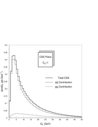
Figure 2: The relative contributions of $q\bar{q}\to t\bar{t}$ and $gg\to t\bar{t}$ to the CSS piece as a function of $Q_{T}$.

We conclude that the $Y$–piece is not important for small $Q_{T}$ up to about 25 GeV, while most of the rate occurs at much smaller $Q_{T}$. In Table 1, we present the rate for the CSS piece alone for $Q_{T}<50$ GeV for each choice of order $(M,N)$ and the dependence of this rate on the renormalization constant $C_{2}$. Results for the $gg\rightarrow t{\bar{t}}$ channel are only presented up to order (1,1). In the same table, we show the mean and standard deviation for each order $(M,N)$. For the highest order, (2,1), the variation with the hard scale set by $C_{2}$ of the $q{\bar{q}}\rightarrow t{\bar{t}}$ channel is only 2%. For the $gg\rightarrow t{\bar{t}}$ channel, there is only a marginal improvement in the variation from higher order, though the overall correction at higher order is large. This raises some concern regarding the higher order dependence of this result. A similar behavior is exhibited in the $gg$ channel for the other resummation schemes. Fortunately, at the Tevatron, the dominant contribution to the $t\bar{t}$ production rate ($\simeq 90\%$) comes from the stable $q{\bar{q}}\rightarrow t{\bar{t}}$ channel. In Fig. 2, we show the relative contributions of the $q\bar{q}$ and $gg$ channels to the CSS piece in this formalism. The total rate for $t\bar{t}$ production is obtained by adding the $Y$–piece to the CSS piece. These results are compiled in Table 2 in a similar fashion as in Table 1. We have also included a column $\alpha_{s}^{(N+2)}\sigma_{pert}$ which shows the LO (for $N=0$) and NLO (for $N=1$) perturbative cross sections for comparison. The choice of order (1,1) for both the $q{\bar{q}}\rightarrow t{\bar{t}}$ and $gg\rightarrow t{\bar{t}}$ contributions represents the same order as the NLO calculation. With the choice of hard scale $Q=M_{t\bar{t}}/2$ ($C_{2}=1/2$), the integrated total production rate for top quark pairs is found to be 5.64 pb, which agrees within 10% with the NLO result 5.06 pb evaluated at the similar hard scale $Q=m_{t}$. This indicates that the CSS resummation formalism presented in the previous section contains the dominant contribution of the NLO result to the production rate of $t\bar{t}$ pairs. Our average resummed result $5.58\pm 0.09$ pb agrees with Ref. [6], which was obtained using principal value resummation. In the literature, the cross section for $t\bar{t}$ production is usually given by taking the hard scale to be a multiple of $m_{t}$ rather than $M_{t\bar{t}}$. For the LO and NLO calculations and other resummation formulations which implicitly integrate out the $Q_{T}$ dependence, the only hard scale left in the problem is the mass $m_{t}$. The LO and NLO perturbative results in the final column of Table 2 are evaluated at the scale $Q=C_{2}\times(2m_{t})$. The scale $Q=m_{t}$, then, corresponds approximately to choosing the renormalization constant $C_{2}=1/2$ in the CSS formalism.

Process	(M,N)	$C_{2}$	$\sigma_{\rm CSS}$ (pb)	${\bar{\sigma}_{\rm CSS}}\pm\delta{\bar{\sigma}_{\rm CSS}}$ (pb)
$q\overline{q}\rightarrow t\overline{t}+X$	(2,1)	1	4.54
		1/2	4.55	4.50$\pm$.07
		1/4	4.42
	(1,1)	1	4.65
		1/2	4.70	4.65$\pm$.05
		1/4	4.60
	(1,0)	1	3.64
		1/2	3.93	3.95$\pm$.32
		1/4	4.28
$gg\rightarrow t\overline{t}+X$	(1,1)	1	0.81
		1/2	0.78	.77$\pm$.05
		1/4	0.71
	(1,0)	1	0.33
		1/2	0.36	.36$\pm$.03
		1/4	0.39

Table 1: CSS Contribution to the Total Cross Section for Top–Antitop Production at the Tevatron

(M,N) for $q{\bar{q}}+gg$	$C_{2}$	$\sigma$ (pb)	${\bar{\sigma}}\pm\delta{\bar{\sigma}}$ (pb)	$\alpha_{s}^{(N+2)}$ $\sigma_{\rm pert}$ (pb)
(2,1)+(1,1)	1	5.51
	1/2	5.49	5.43$\pm$.12
	1/4	5.29
(1,1)+(1,1)	1	5.62		4.71
	1/2	5.64	5.58$\pm$.09	5.06
	1/4	5.47		4.85
(1,0)+(1,0)	1	4.13		3.00
	1/2	4.45	4.47$\pm$.35	4.03
	1/4	4.83		5.57

Table 2: Total Cross Section for Top–Antitop Production at the Tevatron in the CSS Formalism

Our resummation calculation only includes the finite contributions from the virtual diagrams which are the same as those in the Drell–Yan process [11] for the $q{\bar{q}}\rightarrow t{\bar{t}}$ channel and those in Higgs production [15] for the $gg\rightarrow t{\bar{t}}$ channel, plus terms containing the running of $\alpha_{s}^{2}$ in the hard part of the cross section multiplying ${\cal H}_{jk}$. Since there is no final state QCD radiation in the Drell–Yan or Higgs production processes, this is clearly an approximation. If the exact virtual corrections were included, the Wilson coefficient functions $C_{jk}$ would have to be modified in a manner consistent with the CSS formulation, i.e. assuming that the initial and final state gluon radiation for the $t\bar{t}$ process factorizes in a similar fashion as the initial state radiation alone in the Drell–Yan process. While such a factorization is reasonable, there is no formal proof. Therefore, we approximate the $q{\bar{q}}\rightarrow t{\bar{t}}$ ($gg\rightarrow t{\bar{t}}$) finite virtual corrections with those from the Drell–Yan (Higgs production) process. Furthermore, the factor $B^{(2)}$ for $q{\bar{q}}\rightarrow t{\bar{t}}$ inside the Sudakov factor is likely to be different from that for the Drell–Yan process, so we did not include it in our calculations. As shown in Tables 1 and 2, as $C_{2}$ varies between $1/4$ and 1, the total rate varies by only a few percent, which is about the same magnitude as the uncertainty in the NLO calculations. Clearly, all the other finite contributions from the virtual diagrams other than those similar to the Drell–Yan virtual contributions for $q{\bar{q}}\rightarrow t{\bar{t}}$ are small [22]. Since $A^{(2)}$ for this process is the same as for the Drell–Yan process, we have included it in our order (2,1) calculation for $q{\bar{q}}\rightarrow t{\bar{t}}$ to improve our predictions, which yields the results shown in the first row of Table 2.

Because of the agreement of our predictions for the total rate with the NLO calculation, we apply the results of our calculations to study the kinematic distributions of the $t\bar{t}$ pair and the individual $t$ or $\bar{t}$ produced in hadron collisions. In the next section, we present these kinematic distributions and compare them to those predicted by showering event generators. We wish to stress that this is the only type of comparison that is sensible, because the LO calculation predicts a $\delta(\vec{Q}_{T})$ dependence for the $Q_{T}$ distribution, the NLO calculation cannot accurately describe the $Q_{T}\ll m_{t}$ region of phase space, and other resummation formalisms integrate out the $Q_{T}$ dependence and, thus, cannot predict the kinematic distributions of $t$ and $\bar{t}$.

In the following sections, we present results only for order $(2,1)$ and the canonical choice of renormalization constants $C_{2}$=1. There are at least two reasons for doing this. First, the coefficients of the non–perturbative function used in this study were fit to data assuming $C_{2}=1$. While the non–perturbative function can affect the shape of distributions, it does not affect the total rate. Therefore, the stability of our results to variation of $C_{2}$ is still valid, but we cannot trust other choices of $C_{2}$ to give the correct shape. Second, since we do not integrate out the kinematics, we cannot argue that the only scale left in the problem is $m_{t}$. Since an s–channel process dominates, $Q=M_{t\bar{t}}$ is motivated by the dynamics.

We have also checked the effect of neglecting final state radiation, and have found that it reduces the total contribution of the CSS piece to $t\bar{t}$ production by about 10% in our approximation and slightly changes the shape near the peak. Without the final state radiation, however, the $Y$–piece is not finite as $Q_{T}\rightarrow 0$; therefore we include it in our results.

4 Comparison with the Showering Monte Carlo Technique

In this section, we compare our resummed results for the kinematics of the $t\bar{t}$ pair and the individual $t$ or $\bar{t}$ with those predicted by the showering event generator PYTHIA. To make this comparison more understandable, we first explain the approximate implementation of resummation in such generators. The starting point for the showering Monte Carlo technique is the observation that the leading logarithmic singularities in NLO calculations are contained in the Altarelli–Parisi splitting kernels. In this leading log approximation, successive parton emissions occur independently, modulo some angular ordering effects. In a Monte Carlo simulation, which has explicit finite cutoffs for the energy of the emitted radiation, it is possible to treat these emissions as a Markov chain stretching from the hard scattering backwards to the initial state partons [20]. Essentially, one chooses the kinematics for a process at the hard scale $Q_{max}$ based on the LO cross section, then calculates the probability for no parton emission in evolving from a high scale $t_{max}\approx\ln(Q_{max}^{2}/\Lambda_{QCD}^{2})$ to a lower scale $t$. This probability is given in the leading log approximation by the Sudakov form factor $e^{-S(x,t,t_{max})}$, where

$$S(x,t,t_{max})=\int_{t}^{t_{max}}d\acute{t}\sum_{a}\int{d\acute{x}\over\acute{x}}{\alpha_{s}(\acute{t})\over 2\pi}{f_{a}(\acute{x},\acute{t})\over f_{b}(x,\acute{t})}P_{a\rightarrow bc}\left({x\over\acute{x}}\right),$$

$$~{}~{}~{}=\int_{t}^{t_{max}}d\acute{t}\sum_{a}\int{dz}{\alpha_{s}(\acute{t})\over 2\pi}{\acute{x}f_{a}(\acute{x},\acute{t})\over xf_{b}(x,\acute{t})}P_{a\rightarrow bc}(z).$$

Here, $f_{a}(x,t)$ and $f_{b}(x,t)$ are parton distribution functions for partons $a$ and $b$ and $P_{a\rightarrow bc}(z)$ is the Altarelli–Parisi splitting function for the branching $a\rightarrow bc$ with momentum fraction $z$. In improved treatments of the Sudakov form factor, such as in PYTHIA, $\alpha_{s}$ is evaluated not at the scale $Q^{2}$, but at $Q^{2}(1-z)$ [21]. If no radiation occurs down to some cutoff $t_{min}$, $\approx$ 2 GeV in PYTHIA, then the parton is placed on the mass shell. On the other hand, if it is determined that radiation does occur before the cutoff, then a new parton is emitted. The type of branching $a\rightarrow bc$ which led to the parton emission is determined by the relative weights of the $x^{{}^{\prime}}$ integrals over $P_{a\rightarrow bc}$. The initiator of the splitting is given the virtuality $t$, and the process continues until a parton reaches the scale $t_{min}$, and it is placed on the mass shell. With each splitting, the remaining kinematics are sampled so that energy and momentum are conserved. The result is a total cross section given by the LO calculation, but with the kinematic distributions of a resummed calculation. In this sense, it corresponds to a choice of $(M,N)=(1,0)$ in the CSS formalism. Final state radiation is implemented in a similar fashion, but it occurs forward from the hard scattering process to the final state and is not weighted by the parton distribution functions.

First, we present a comparison of the resummed and showering Monte Carlo kinematics for the $t\bar{t}$ pair. Several observables which in principle cannot be extracted from a NLO calculation are the distributions of the transverse momentum of the $t\bar{t}$ pair $Q_{T}$, the opening angle between $t$ and $\bar{t}$ in the azimuthal plane $\Delta\phi_{t\bar{t}}$, and the variable $z\equiv-{{\vec{p}_{T}}(t)\cdot{\vec{p}_{T}}({\bar{t}})\over|max({p_{T}^{2}}(t),{p_{T}^{2}}({\bar{t}}))|}$. The resummed results are separately shown as solid lines. Displayed on the same plots are the shapes predicted by PYTHIA for two choices of hard scale, $Q^{2}=\hat{s}$ and $Q^{2}=\sqrt{m_{t}^{2}+p_{T}^{2}}$, where $p_{T}$ is the transverse momentum of the top quark at LO. As illustrated in Table 2, the LO rate is highly sensitive to the choice of hard scale. The resummed estimate of the total rate is more reliable. Therefore, to compare the shapes of distributions, we have renormalized the PYTHIA results to have the same total rate as the resummed calculation.

Fig. 3 shows the distribution of the resummed variable $Q_{T}$. Note that the resummed distribution is significantly harder than the showering Monte Carlo result, implying that the resummed calculation predicts more overall hard radiation. This is further demonstrated by the $\Delta\phi_{t\bar{t}}$ distribution, the difference in azimuthal angle between $t$ and $\bar{t}$, in Fig. 4, which is depleted near $\Delta\phi=\pi$ in comparison to the showering Monte Carlo. Because of initial or final state radiation, the $t$ and $\bar{t}$ are not expected to be exactly back–to–back. The $z$ distribution, shown in Fig. 5, is also shifted away from a back–to–back configuration $(z=1)$ in the resummed result. Finally, the distributions of the rapidity of the $t\bar{t}$ pair $y_{t\bar{t}}$ and the invariant mass $M_{t\bar{t}}$ are shown in Figs. 6 and 7 respectively. The rapidity distribution is more central for the resummed result and the invariant mass favors higher masses and is broader. These differences arise because PYTHIA only contains LO matrix elements, while the resummed result contains the dominant piece of the NLO correction.

Second, we present a comparison of the kinematics of the individual $t$ or $\bar{t}$. Fig. 8 shows the distribution of the transverse momentum of the individual $t$ $p_{T}^{t}$, while Fig. 9 shows the difference in their rapidity $\Delta y^{t}$, where $\Delta y^{t}=y^{t}-y^{\bar{t}}$. From the LO calculation, we know the scale of $p_{T}^{t}$ is set by $m_{t}$ ($p_{T}^{t}\simeq m_{t}/3\simeq$ 60 GeV), while the typical transverse momentum $Q_{T}$ is much smaller. Therefore, there is not much difference in these distributions. Likewise, $\Delta y^{t}$ is more sensitive to the PDF (which determines the boost of the $t\bar{t}$ pair) than the transverse momentum $Q_{T}$, so we do not expect to observe a large difference. In conclusion, the showering generators (as typified by PYTHIA in our study) reproduce the CSS distributions for the individual $t$ and $\bar{t}$ and the $t\bar{t}$ pair kinematics in our plots to a 10% level bin–by–bin, although the overall shapes are generally different and the complete resummed results indicate more overall hard radiation. Based on these results, we seek to improve the showering Monte Carlo technique by using our knowledge of the resummed $Q_{T}$ distribution. This is discussed in the next section.

5 Jet Activity in $t\bar{t}$ Events at Hadron Colliders

Despite its limitations in predicting the correct rate, the showing Monte Carlo technique has a mechanism to approximate the complete resummed result for the $Q_{T}$ distribution. Furthermore, the showering event generator gives a phenomenologically accurate description of all the details of the event. The resummation calculation only predicts the vector sum of all soft gluon radiation, but has no power to predict how the radiation is distributed amongst individual gluons or quarks. Such details are crucial for estimating the amount of jet activity, which will affect the determination of the top quark mass by reconstructing jets from top quark decays as done by CDF and D0 at the Tevatron [1]. These estimates are used to engineer cuts to enhance the signal and to optimize the choice of jet definition. In this section, we present a simple synthesis of the showering Monte Carlo technique and the full resummation calculation to realize a better estimate of the hadronic activity. This synthesis is accomplished by reweighting events generated by PYTHIA to agree with the resummed $Q_{T}$ distribution and rate.

To demonstrate the improved predictive ability of the resummed approach, we present the distributions of the jet multiplicity and scalar sum of the transverse energy in $t\bar{t}$ events. We have isolated the contributions from initial and final state radiation only, so that none of the the $t$ or $\bar{t}$ decay products (or additional QCD radiation contributions from them) are included in these plots. We define jets using a simple calorimeter simulation (with cell segmentation $\Delta\eta\times\Delta\phi=.1\times.1$) and a clustering algorithm based on a cone size $R=.4$ and a minimum jet transverse energy $E_{T}^{min}$=5 GeV. The energy $E$ deposited in each cell of the calorimeter is smeared with a Gaussian resolution ${\sigma_{E}\over E}={.70\over\sqrt{E}}$. The jet multiplicity distribution is shown in Fig. 10. Note the shift in the peak value of the distribution from 0 jets to 1 jet. The resummation based Monte Carlo clearly predicts more hard radiation in $t\bar{t}$ events at hadron colliders. Similar information is conveyed in Fig. 11, which shows the scalar sum of the transverse energy of the jets defined as above. While the details of jet observables can only be studied using the showering Monte Carlo technique, our knowledge of the resummed $Q_{T}$ distribution allows improvement. It is straightforward to extend these results to include the decay products of the $t$ and $\bar{t}$ and even the hard gluons from the QCD radiative decay of the top quark [23]. We shall leave this for further study.

As a final point of comparison, we have attempted to quantify the effect of hard gluon radiation on the extraction of $m_{t}$ from data. The issue at hand is how often a hard gluon from radiation is misidentified as a top quark decay product. Using a sample of events where $t(\to bW^{+}(\to e^{+}\nu_{e})){\bar{t}}(\to{\bar{b}}W^{-}(\to jj))$, we cluster particles into jets as described above and analyze events with 4 or more hard jets ($E_{T}^{j}>$15 GeV, $|\eta^{(j)}|<2$). We separate the jets than can be identified with a $\bar{t}$ decay product (for simplicity, we assume the $b$ is correctly tagged) and find the one with the lowest $E_{T}$. The fraction of events where another jet (i.e. one not from $\bar{t}$ decay) has a higher $E_{T}$ than this is an estimate of the importance of the hard radiation. While this is only a crude estimate of the real effect, we find that the fraction ($=.56$) does not differ between the standard and improved PYTHIA. This implies that the hard gluon error on the top mass measurement is well estimated by showering generators, though this requires further study. We have not attempted to quantify the effect of soft gluon radiation, where the radiation is not resolved as an individual jet but can overlap with the $t\bar{t}$ decay products, though the complete resummed result indicates that this too should be enhanced.

6 Conclusions

To further study the interactions of the top quark and to better measure its mass, we must understand the kinematic distributions of the transverse momentum, rapidity and azimuthal angle of the top quarks. The kinematics of the top quarks produced at hadron colliders can be accurately predicted only after resumming the multiple soft gluon emissions in either the initial state or the final state. In this work, we have adopted the CSS resummation formalism to obtain the kinematics of the top quarks. The approximation we made in this study should be adequate because of the large top quark mass. The important consequence of the large top quark mass is that the logarithmic terms from the initial state are more important than those from the final state. In the former case, there is double–logarithmic behavior due to both soft and collinear gluon radiation, while, in the latter case, only single-logarithmic behavior due to soft but not collinear gluon radiation is possible up to the order $\alpha_{s}^{3}$. We compared our resummation calculation with those predicted by the full event generator PYTHIA and found that the latter does not give the same prediction as ours. In view of the fact that the full event generator has been widely used by our experimentalist colleagues for analyzing their data, it is important to point out the difference between the results from this approach and those from the analytical calculation. In determining the mass of the top quark, for example, one needs to account for the jet activity in at least two cases: (1) when a hard jet from the showering is misidentified as one of the top decay jets, and (2) when the soft radiation is included in the energy determination of true top decay products. The hybrid approach presented in Section 5, which relates the transverse momentum of the top–antitop quark pair from an analytic calculation to the balancing gluon radiation from a showering Monte Carlo, contains a more realistic description of event structure, which could be used for choosing kinematic cuts and tuning the jet energy correction algorithm.

Figure 1: The relative importance of the $Y$-piece with respect to the CSS piece as a function of $Q_{T}$.

Figure 3: The transverse momentum of the ${t\bar{t}}$ pair $Q_{T}$ for $C_{2}$=1 and for different choices of hard scale for the showering Monte Carlo PYTHIA. The PYTHIA rate has been renormalized to the CSS rate.

Figure 4: The difference in azimuthal angle between the $t$ and $\bar{t}$ $\Delta\phi_{t\bar{t}}$.

Figure 5: $z$ distribution of the $t$ and $\bar{t}$.

Figure 6: Rapidity of the $t\bar{t}$ pair $y_{t\bar{t}}$.

Figure 7: Invariant mass of the $t\bar{t}$ pair $M_{t\bar{t}}$.

Figure 8: Transverse momentum of the individual $t$ or $\bar{t}$ $p_{T}^{t}$.

Figure 9: Rapidity difference between the $t$ and $\bar{t}$ $\Delta y_{t}$.

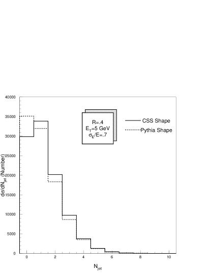
Figure 10: Jet Multiplicity from initial and final state radiation as predicted by PYTHIA (dashed line) and the hybrid PYTHIA– CSS resummation (solid line).

Figure 11: Scalar sum of jet transverse energy $\sum E_{T}$ from initial and final state radiation as predicted by PYTHIA (dashed line) and the hybrid PYTHIA– CSS resummation (solid line).

References

-
[1]
F. Abe et al., Phys. Rev. Lett. 73, 225 (1994);
S. Abachi et al., Phys. Rev. Lett. 72, 2138 (1994). - [2] Ehab Malkawi and C.–P. Yuan, Phys. Rev. D50, 4462 (1994).
- [3] R.S. Chivukula, E. Gates, E.H. Simmons and J. Terning, Phys. Lett. B311, 157 (1993);
-
[4]
P. Nason, S. Dawson and R.K. Ellis,
Nucl. Phys. B303, 607 (1988); B327, 49 (1989);
W. Beenakker, H. Kuijf, W.L. van Neerven and J. Smith, Phys. Rev. D40, 54 (1989);
R. Meng, G.A. Schuler, J. Smith and W.L. van Neerven, Nucl. Phys. B339, 325 (1990). - [5] E. Laenen, J. Smith and W.L. van Neerven, Nucl. Phys. B369, 543 (1992).
- [6] E.L. Berger and H. Contopanagos, Phys. Lett. B361, 115 (1995).
- [7] S. Catani, M.L. Mangano, P. Nason and L. Trentadue, CERN-TH/96-21, January 1996.
- [8] G. Altarelli, R.K. Ellis, M. Greco, G. Martinelli, Nucl. Phys. B246, 12 (1984).
- [9] E.L. Berger and R. Meng, Phys. Rev. D49, 3248 (1994).
- [10] J. Collins and D. Soper, Nucl. Phys. B193 381, (1981); Erratum B213 (1983) 545; B197, 446 (1982).
- [11] J. Collins, D. Soper and G. Sterman, Nucl. Phys. B250, 199 (1985).
- [12] G. Marchesini, B.R. Webber, G. Abbiendi, I.G. Knowles, M.H. Seymour, and L. Stanco, Comp. Phys. Commun. 67, 465 (1992); H. Baer, F. Paige, S. Protopopescu, and X. Tata, ”Simulating Supersymmetry with ISAJET 7.00,” FSU–HEP–930329, SSCL–Preprint–441 (1993); T. Sjöstrand, Comp. Phys. Commun. 82, 74 (1994).
- [13] S. Frixione, M.L. Mangano, P. Nason, and G. Ridolfi, Phys. Lett. B351, 555 (1995).
- [14] P.B. Arnold and R.P. Kauffman, Nucl. Phys. B349, 381 (1991).
- [15] C.-P. Yuan, Phys. Lett. B283, 395 (1992).
- [16] R.P. Kauffman, Phys. Rev. D45, 1512 (1992).
- [17] J. Collins and D. Soper, Phys. Rev. D16, 2219 (1977).
- [18] H.L. Lai, J. Botts, J. Huston, J.G. Morfin, J.F. Owens, J.W. Qiu, W.K. Tung, H. Weerts, MSU preprint MSU-HEP-41024, Oct 1994.
- [19] G.A. Ladinsky and C.-P. Yuan, Phys. Rev. D50, 4239 (1994).
- [20] T. Sjöstrand, Phys. Lett. 157B, 321 (1985).
- [21] A. Bassetto, M. Ciafaloni and G. Marchesini, Phys. Rep. 100, 202 (1983).
- [22] R. Meng, G.A. Schuler, J. Smith, and W.L. van Neerven, Phys. Lett. B339, 325 (1990).
- [23] S. Mrenna and C.-P. Yuan, Phys. Rev. D46, 1007 (1992).