Abstract
We have investigated some observable consequences of colour reconnection in the reaction $\mathrm{e}^{+}\mathrm{e}^{-}\rightarrow\mathrm{W}^{+}\mathrm{W}^{-}\rightarrow\mathrm{q}_{1}\overline{\mathrm{q}}_{2}\mathrm{q}_{3}\overline{\mathrm{q}}_{4}$. We use a measure based on the momentum structure of the event, comparing reconnected events with ‘standard’ ones. Some different recoupling models are described and studied as well as simpler toy models to show where the effects are present and what makes most of them disappear in realistic models. Some attempts are made to introduce suitable cuts in order to select the interesting events.

1 Introduction

The reaction $\mathrm{e}^{+}\mathrm{e}^{-}\rightarrow\gamma^{*}/\mathrm{Z}^{0}\rightarrow\mathrm{q}\overline{\mathrm{q}}$ is well known and has been studied for some time, for example at LEP at CERN, where the $\mathrm{Z}^{0}$ has been produced at roughly 90 GeV energy. This reaction is well described by QCD in the perturbative (shower) region and the Lund string model [1] in the non perturbative (fragmentation) one. In the Lund model strings are drawn between the quarks, possibly via radiated gluons. The strings can be seen as colour flux tubes or vortex lines. The subsequent fragmentation of a string will produce the observed particles. Events generated in this manner with the Jetset and Pythia programs [2] have successfully described many observed phenomena. A summary of the experience from LEP1 is given in [3], where a discussion of the extrapolation to LEP2 energies is also given. The reaction of primary interest to us in this work is:

$$\mathrm{e}^{+}\mathrm{e}^{-}\rightarrow\mathrm{W}^{+}\mathrm{W}^{-}\rightarrow\mathrm{q}_{1}\overline{\mathrm{q}}_{2}\mathrm{q}_{3}\overline{\mathrm{q}}_{4}~{}.$$ (1)

One of the goals of LEP2 is to study this reaction experimentally from the threshold at 160 GeV onwards. This experiment starts this year and will go on for the rest of the century. Some ten thousand events should be observed at LEP2, but not all will be of interest to us, so the low statistics will be a big problem when we want to apply our methods on future experimental data. We are for example not interested in events that produce leptons, and we also need to introduce certain cuts that further limit the number of surviving events.

A first attempt to describe the reaction (1) would be to assume that the $\mathrm{q}\overline{\mathrm{q}}$-pair from $\mathrm{W}^{+}$ forms one colour singlet and that the $\mathrm{q}\overline{\mathrm{q}}$-pair from $\mathrm{W}^{-}$ forms a second one, and then the two systems shower and fragment independently of each other like two overlapping $\mathrm{Z}^{0}$ decays at LEP. The $\mathrm{W}$-particles, however, exist only for a very short time, therefore the space–time separation between the production points of the two $\mathrm{q}\overline{\mathrm{q}}$-pairs is very small. In one extreme case you could assume that all four quarks are produced at the same point. Thus, in addition to the original colour dipoles $\mathrm{q}_{1}\overline{\mathrm{q}}_{2}$ and $\mathrm{q}_{3}\overline{\mathrm{q}}_{4}$, it would be possible to form another set of dipoles, namely $\mathrm{q}_{1}\overline{\mathrm{q}}_{4}$ and $\mathrm{q}_{2}\overline{\mathrm{q}}_{3}$. In the framework of the Lund model this would mean that the fragmenting strings should be drawn differently depending on what quarks form the dipoles. It is not unreasonable to assume that this should give observable effects in the final state.

The possibility of colour reconnection has been studied before, for example in [4] where a simple ‘instantaneous’ reconnection scenario is discussed. The rearranged dipoles are here supposed to form immediately and then shower and fragment independently of each other. Under ideal geometrical conditions the effects can be very large, but it has been shown that the distance between the decay vertices of the W-particles is large enough for perturbative QCD-radiation in the original dipoles to occur independently of each other in a first approximation [5]; therefore the instantaneous scenario is not very realistic. The non-perturbative phase, however, extends much further in space so here the possibility of colour rearrangement is much larger. A summary of the different models is given in [6].

In [5] several more or less realistic models for non-perturbative reconnection have been proposed. These will be described in more detail in section 2 and are those primarily studied in this work. Gustafson and Häkkinen [7] have another approach where they draw the strings in such a way that the potential energy of the strings (lambda-measure) is minimized. In this way differences between reconnected and ‘normal’ events can be seen, barely, in the rapidity distribution of charged particles. Since this signal is indirect, we here propose a method which will allow a more direct study of the string topology.

In this work we will study an observable constructed from the momentum of the hadrons in the final state. Well-behaved four-jet events are studied, the jets paired two by two in all possible ways and each pair is boosted to the system where the jet pairs are back-to-back. In this system the sum of the transverse momenta of the particles belonging to the pair is calculated. If there is a string between the quarks supposed to be mothers of these jets the sum should be minimized. The method will be discussed further in sections 2 and 3 where it will be applied to three-jet and four-jet events in $\mathrm{Z}^{0}$ decays.

The main reasons to study the effects of colour reconnection are the possibility to determine the structure of the QCD vacuum and to find possible systematic errors in the measurement of the mass of the $\mathrm{W}$ particle. Models based on superconductivity have been proposed in e.g. [4] and [5], where the strings are supposed to behave like either Type I or Type II superconductors. The goal is to study different distributions for the reconnection models and find differences between these. In the end the distributions could be compared to experiment in order to either verify or reject the models. In this work small observable differences have been discovered in the more realistic models, but we also study some simpler toy models and note that the effects can be quite significant. We therefore analyze where the effects diminish.

2 Theoretical overview

Let us study the reaction (1) in a little more detail to better understand the different reconnection models. The process can roughly be divided into the following stages:

• $\mathrm{e}^{+}\mathrm{e}^{-}$ annihilation and $\mathrm{W}^{+}\mathrm{W}^{-}$ production;

• weak $\mathrm{W}^{+}\mathrm{W}^{-}$ decay to quarks and leptons;

• parton shower;

• fragmentation (hadronization);

• unstable particles decay into the observed particles.

The annihilation of electrons and positrons is a very clean process in the sense that both the initial and final states consist of structureless particles. The experimental situation is also simplified by the fact that the reaction takes place in the laboratory rest-frame. Figure 1 gives some examples of possible reactions. The black blobs are there to emphasize that several graphs contribute to the matrix element for this reaction.

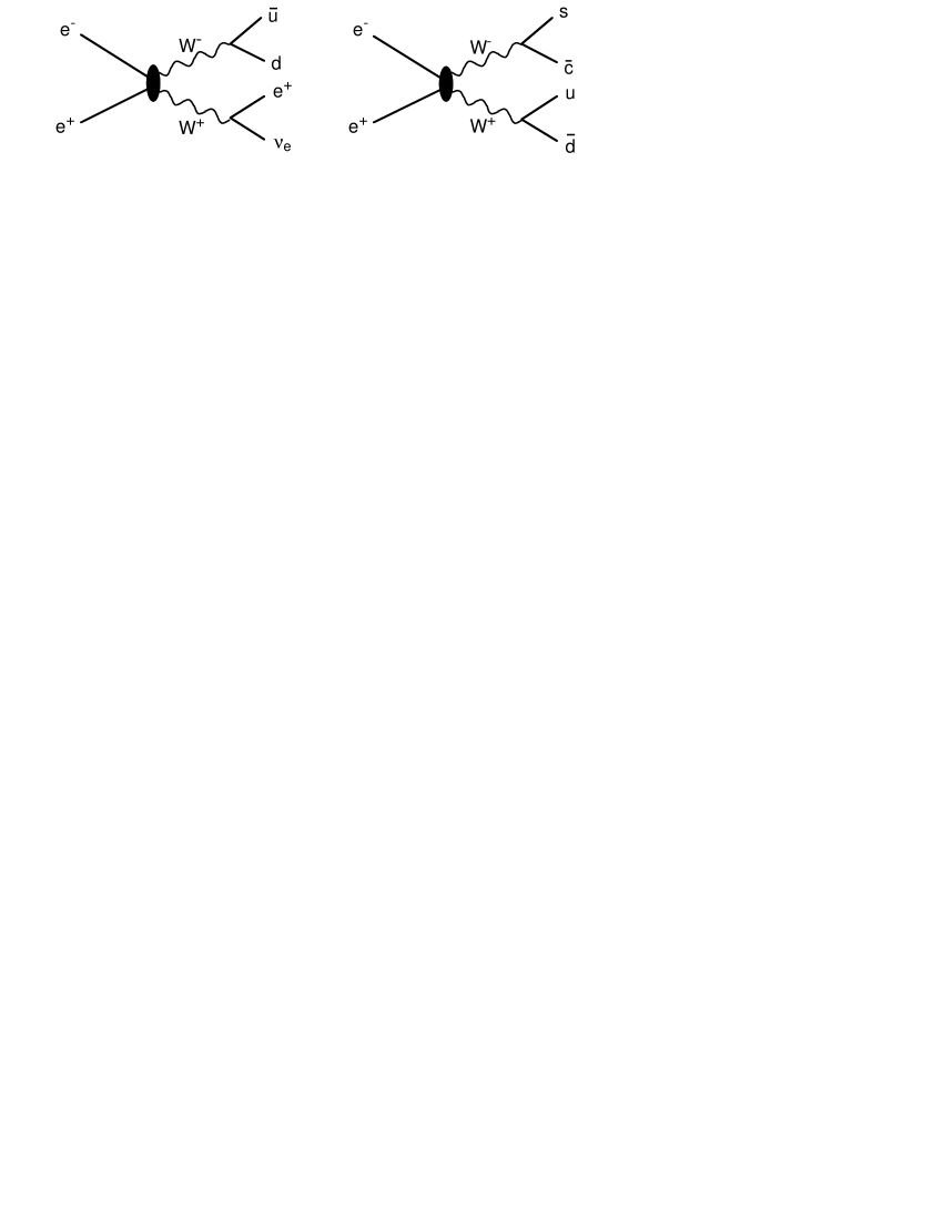
Figure 1: Some examples of the reaction $\mathrm{e}^{+}\mathrm{e}^{-}\rightarrow\mathrm{W}^{+}\mathrm{W}^{-}\rightarrow$leptons and quarks.

2.1 No reconnection scenario

The W-particles live for a very short time and the separation between their decay points is less than 0.1 fm ($10^{-16}$ m). The W boson has several decay modes. The only one that interests us is $\mathrm{W}\rightarrow\mathrm{q}\overline{\mathrm{q}}$. Assuming quark–lepton symmetry, no quark mixing, and the fact that the top-quark is much heavier than the $\mathrm{W}$-particle, approximately 45% of the $\mathrm{W}^{+}\mathrm{W}^{-}$ events produce two quark–antiquark pairs.

Figure 2: Simplified parton showers. Curly lines are gluons.

Then each quark-antiquark pair is allowed to radiate other quarks and gluons via the basic branchings $\mathrm{q}\rightarrow\mathrm{q}\mathrm{g}$, $\mathrm{g}\rightarrow\mathrm{g}\mathrm{g}$, and $\mathrm{g}\rightarrow\mathrm{q}\overline{\mathrm{q}}$. In this region the particles are highly virtual and the distances are very small (less than 1 fm), so perturbative QCD is applicable. This shower is cut off at some lower virtuality scale $Q_{0}\approx$ 1 GeV. A simplified shower is shown in figure 2. It will turn out that this stage blurs out most of the effects of colour reconnection.

When the quarks are more than about 1 fm apart perturbation theory breaks down and different models are used to describe the fragmentation process. We use the standard Lund model where strings are drawn between partons with opposite colour charges. Figure 3 shows some typical string configurations and the colours of the different partons. The term ‘parton’ is a collective term for quarks and gluons. The string could be seen as a force field that is essentially one-dimensional. This arises from the unique properties of QCD where the gluon self coupling makes the field lines want to stick together, unlike QED where the field lines spread throughout all space. In such a one-dimensional field the force would not depend on the separation between the partons, so the energy in the colour field increases approximately linearly with the distance between the quarks. Within this colour flux tube new $\mathrm{q}\overline{\mathrm{q}}$-pairs can be created from the increasing field energy. This fragmentation goes on until only ordinary hadrons remain. Some of these hadrons may be unstable and decay further into the stable hadrons, leptons and photons that are actually observed. $p_{\perp}$, the transverse momentum of the produced hadrons relative to the string direction, fluctuates and has an approximately Gaussian spectrum.

Figure 3: Example of string configuration. Only colours are shown in the picture, r=red, g=green, b=blue. Dashed lines are strings.

Most of what has been described so far, $\mathrm{W}^{+}\mathrm{W}^{-}$ production, quarks, parton shower, fragmentation, and decay are never directly observed. What is seen in the detector is the stable particles produced in the reaction. The number of observed particles varies a lot from event to event but it is in the order of 50. The particles are not distributed isotropically over all angles, instead they are clearly collected in two or more narrow sprays of particles. Therefore the concept of jets is introduced, where particle momentum is summed up according to different clustering algorithms so as to better reflect the direction of the parent quarks. In order to be able to compare results with experiment we mainly use observable quantities in our analysis. Sometimes, however, we use the benefits of having a Monte Carlo ‘behind the scene’ view to test our results.

Consider next the momentum structure of the jets and strings, specifically the back-to-back system of a jet pair with a string between them. The momenta of the individual particles that constitute the jets are not necessarily parallel to the direction of the jets but most of them are almost aligned, because the particles are the remains of the fragmented string drawn between the $\mathrm{q}\overline{\mathrm{q}}$-pair. In momentum space the particles in the rest frame are distributed along a hyperbola as in figure 4(a). The directions of the quarks are in the asymptotes of the hyperbola. If the system is boosted to the back-to-back system the momenta of the particles constituting the jet will be almost aligned to the jet axis as in (b). In a real jet the transverse momentum fluctuates slightly and gives a smeared out picture as is indicated by the lines in the figure. If the quarks belonging to the back-to-back jets do not have a string drawn between them they will not follow a hyperbola and will be more spread out in the back-to-back system. We will be interested in this broadening in our event analysis.

Figure 4: Momentum structure of the jets. a Lab system b Back-to-back system. Fluctuations are represented by the horizontal lines.

2.2 Colour reconnection

If we imagine that the $\mathrm{W}^{+}$ and $\mathrm{W}^{-}$ systems shower and fragment independently of each other we would have no problem. Then the produced hadrons are, in theory, uniquely assigned either to the $\mathrm{W}^{+}$-system or to the $\mathrm{W}^{-}$-system. The $\mathrm{W}$-particles decay very close to each other both in space and time, however, so this kind of separation might not be possible. It is therefore useful to discuss the wavelength of gluons in different stages of the process. A hard gluon in the perturbative region has a wavelength much smaller than the decay vertex separation and can therefore resolve the two decay vertices. Indeed, it has been shown [5] that QCD interference effects are negligible for energetic gluon emission involving energies significantly larger than $\Gamma_{\mathrm{W}}$. In the fragmentation region, on the other hand, gluon wavelengths are much larger and interference effects should be more important. Having said this we concentrate on the possibility of reconnection in the non-perturbative fragmentation region where the typical distance a parton travels before branching, in the parton shower picture, is larger than the $\mathrm{W}^{+}\mathrm{W}^{-}$ separation.

As has been mentioned before, the complexity of QCD prohibits a description of the fragmentation process from first principles so that reconnection in this phase has to be modelled too. Several different models has been proposed and they all build on different assumptions about the QCD vacuum. The ones studied in this work are:

1. Reconnection at origin of event. A simple ‘instantaneous’ model where strings are always reconnected. Reconnection before shower and fragmentation. Not considered to be realistic.

2. Same as above but with reconnection after shower but before fragmentation. The ‘intermediate’ model. The simplest of the more realistic models.

3. Reconnection when strings overlap based on cylindrical geometry. A ‘bag model’ based on a type I superconductor. The reconnection probability is proportional to the overlap integral between the field strengths. The field strength has a Gaussian fall-off in the transverse direction, and a radius of about 0.5 fm. The model contains a free strength parameter that can be modified to give any reconnection probability.

4. Reconnection when strings cross. In this model the strings mimic the behaviour of the vortex lines in a type II superconductor where all topological information is given by a one-dimensional region in the core of the string.

5. In this model strings are drawn between partons in such a way that the ‘length’ is minimized. As a measure of this length a so called $\lambda$-measure is used. This can also be seen as a measure of the potential energy of the string.

These models will be referred to by their number or by their name. Models 1 through 4 is described in great detail in [5] and the last in [7]. Models 1 and 2 will also be studied without parton showers as toy-models.

Colour reconnection is not limited to $\mathrm{W}^{+}\mathrm{W}^{-}$ decays. It has been studied in other reactions as well, for example in the decay $\mathrm{B}\rightarrow\mathrm{J}/\psi+X$ where colour reconnection is needed to create the observed $\mathrm{J}/\psi$-particle. The $\mathrm{B}$-meson contains a $\mathrm{b}$-quark and the $\mathrm{J}/\psi$ is a $\mathrm{c}\overline{\mathrm{c}}$ state. In the underlying decay $\mathrm{b}\rightarrow\mathrm{c}\mathrm{W}^{-}\rightarrow\mathrm{c}\overline{\mathrm{c}}\mathrm{s}$ the natural colour singlet would be $\mathrm{s}\overline{\mathrm{c}}$ and only in 1/9 of the cases would $\mathrm{c}\overline{\mathrm{c}}$ be a possible singlet system. Without the possibility of colour reconnection the production of $\mathrm{J}/\psi$ would be more suppressed than it has been observed to be. Other examples are mentioned in [5].

3 Method of analysis

In this section we present the method used to study colour reconnection. We first describe the principle behind the method and then apply it to the reaction:

$$\mathrm{e}^{+}\mathrm{e}^{-}\rightarrow\mathrm{Z}^{0}\rightarrow\mathrm{q}\overline{\mathrm{q}}\rightarrow\mathrm{q}\overline{\mathrm{q}}\mathrm{g}$$ (2)

where a hard gluon is emitted by the initial $\mathrm{q}\overline{\mathrm{q}}$-pair. This reaction typically produces a three-jet event where one jet is associated with the gluon and the other two with the quarks. We use this, as a test of our method, to identify the gluon jet. A second example involving four-jets is also studied in a simple case. In section 4 we proceed with the study of reaction (1), where we want to find out how the strings are drawn using different methods and different recoupling models.

3.1 The $p_{\perp}$ minimization method

We consider an event producing a few well separated jets that can be paired one-to-one with the same number of initial quarks or hard gluons. Then we consider the possible string configurations and try to find out what configuration has been realized in a specific event. In the first example that we study, reaction 2, there is only three possible string configurations with two strings in each. Therefore we set up three hypotheses and proceed to find the right one by looking at the back-to-back system of every pair of jets that are assumed to have strings between them. In this system $\sum{p_{\perp}}$— the sum of the transverse momentum of the particles that ‘belong’ to this jet pair — is calculated. How a particle is assigned to a jet pair depends on the situation, but in principle a particle is assigned to the jet pair in whose back-to-back system its $p_{\perp}$ is minimized. This will be made clear in the specific examples. The ‘right’ hypothesis is then identified as the one that minimizes $\sum{p_{\perp}}$. Why this is so will be explained and shown in the following sections.

3.2 Test of the method in three-jet events

We demonstrate this method by studying the reaction (2) where the three hypotheses are depicted in figure 5. In this case, because of conservation of momentum, the reaction takes place in a single plane. This simplifies the analysis somewhat. In (a) jet 1 is assumed to be the gluon; therefore strings are drawn between the quarks via jet 1. Alternatively the gluon can be seen as a kink on the string between the quarks.

All particles to the left of the dashed line are assigned to the left string and all particles right of the line to the right one. Then two boosts are performed. One to the back-to-back system of jet 1 and 2 and one to that of 1 and 3. In each of these systems $\sum{p_{\perp}}$, for the ‘right’ and ‘left’ particles respectively, is calculated and the sums are added together. The number obtained in this way is a measure of the ‘goodness’ of the hypothesis: the smaller the $\sum{p_{\perp}}$ is the better particles are lined up along the expected hyperbola, compare figure 4. The same is done in (b) and (c) but in these cases the gluon is assumed to be in the direction of jet 2 and 3 respectively.

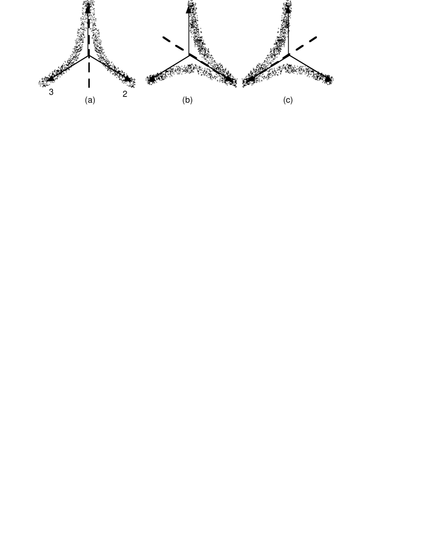
Figure 5: The three different hypotheses. The arrows show the direction of the jets. The gluon is giving rise to: a jet1 b jet2 c jet3. The smearing shows the expected momentum distribution in the respective hypothesis.

Because of the way the momentum of the particles is distributed when a string is drawn between jets – in the ideal case along a hyperbola – the right hypothesis should be the one with the smallest $\sum{p_{\perp}}$. Imagine for example that (a) is the right hypothesis but we make the cut and boosts according to (b). When we boost to the 2-3 system, the transverse momenta of particles not aligned to a hyperbola in the rest-frame will be exaggerated and $p_{\perp}$ will increase.

We test this method by generating $\mathrm{Z}^{0}\rightarrow\mathrm{q}\overline{\mathrm{q}}$ events at 91.2 GeV using the Jetset 7.4 and Pythia 5.7 event generators [2]. We generate standard events but switch off initial state photons and leptonic $\mathrm{Z}^{0}$ decays. Using the clustering algorithm in Jetset we search for three-jet events and perform the analysis described above to identify the gluon jet with our method. In a Monte Carlo simulation it is possible to trace the showering of the primary $\mathrm{q}\overline{\mathrm{q}}$-pair and find the momenta of the original quarks after the parton shower. Then we check the direction of the jets and match two of them with the quarks. The last jet is assumed to come from a hard gluon. In this way we can see how often we get the ‘right’ answer when using this method. In a real experimental event this would of course not be possible, other techniques have to be used to tag the gluon-jet. Had the methods been completely uncorrelated we would be right in 33 % of the cases. As it turns out we are right in more than 50 % and under ideal conditions we get over 80 %, see table.

For better results we have some parameters that we can change. These are:

• $d_{\mathrm{join}}$ in the clustering algorithm. This is a distance scale in GeV above which two clusters may not be joined. It can be said to control the jet-resolution power. A higher number makes the algorithm more prone to join two jets and hence a three-jet could be classified as a two-jet if $d_{\mathrm{join}}$ is too large. For small numbers it is the other way around.

• Particle energy cut. Particles with high energy and hence large momentum should not contribute as much to the difference between jet-pairs with and without strings, since the string hyperbolae run almost parallel to the jet directions at large momenta, compare figure 5.

• Jet energy cut. If one of the reconstructed jets has a small energy it could be that no hard gluon is associated with this jet and the event should therefore not be part of the analysis.

• The angle between any two jets should be above some minimum value. This one is not varied but held constant at $60^{\circ}$.

These parameters are arguably not all independent and it is not our intention to optimize the cuts, nevertheless in table 1 some results are shown for different values of the parameters.

run	$d_{\mathrm{join}}$	jet-energy	particle-energy	% ‘right’	% considered
1	3.5	8.0	2.0	58	17
2	3.5	8.0	4.0	64	17
3	3.5	8.0	10.0	63	18
4	5.5	8.0	4.0	61	23
5	5.5	12.0	4.0	58	18
6	5.5	16.0	4.0	54	13
7	7.5	8.0	4.0	57	22
8	7.5	16.0	4.0	52	13
9	2.0	12.0	4.0	57	2.0
10	7.5	4.0	15.0	87	100

Table 1: Run 1–8 and 10: 20,000 generated events. Run 9: 100,000 events and optimal cuts, a small percent of considered events is not really a problem because of the good availability of data. All units are in GeV, jet-energy is lower limit while particle-energy is upper limit. The last item is results from ideal conditions as described in the text.

Statistics is not really a problem in the case of reaction (2). There exists data from millions of experimental events at LEP which enables us to study as many events as we like in order to get only a small statistical error. In table 1, run 1–6, events with different cuts are divided into groups of three where only one parameter is varied. The predictive power of the method is given by the percentage in column 5. The ‘% considered’ should be somewhere around 10% from the known amount of three-jets in this reaction. Some conclusions could be drawn from this: The ‘% right’ is only moderately sensitive to the cuts in $d_{\mathrm{join}}$, jet-energy and particle-energy. The cut in jet-energy should be in the larger region to get fewer considered events. Row 9 shows ‘optimized’ cuts and has a very low $d_{\mathrm{join}}$ (default is 2.5 GeV) and high jet-energy cut. A low value of $d_{\mathrm{join}}$ will force the clustering algorithm to pick out clear three-jets only and hence enhance the results.

In a ‘real life’ event generation like in 1–9 of table 1 fluctuations play a significant part in the results.The gluon-jet, for example, is almost never as pronounced as in figure 5 and the jet-axis is not exactly aligned to the direction of the quarks and gluons. This will make the alignment of momentum to the hyperbola uncertain and $\sum{p_{\perp}}$ might become larger. In order to see clearly that the method is correct we generate events with a $\mathrm{u}\overline{\mathrm{u}}$-pair and a gluon, each with one third of the total center of mass energy, aligned in a plane with equal angles. The result from this is shown in run 10 of table 1. Here the particles are collected to begin with so it is better to increase $d_{\mathrm{join}}$ to get as many three-jet events as possible (in this case 100%, see table).

3.3 Four-jet events

In a three-jet event with planar structure like the one in figure 5 it has been shown that the region between the quark-jets contains less particles than the other two does. This result is in good agreement with the Lund string fragmentation model but not with independent fragmentation. In the independent fragmentation model the partons fragment independently of each other and no string effects should be noticed. This is discussed in [1] where experimental as well as theoretical results are cited.

No similar study has been made in four-jet events, no doubt due to the difficult geometry. It could be possible to do this by using the described $p_{\perp}$-method. Here we study only a very simple example where the initial quark-gluon configuration is depicted in figure 6a. This configuration is then allowed to fragment according to the two different fragmentation models (Lund and independent). Four jets are constructed and in this case there are twelve different ways to draw the strings between the four jets. First there are six ways to choose which two jets belong to the quark and anti-quark and for each of these there are two possible ways to draw the strings via the gluons. Three of these twelve string configurations are shown in figure 6(b, c and d), where (b) and (c) corresponds to the parton configuration in (a) while (d) corresponds to a configuration where the quarks and gluons change places. The rule is that each quark must have only one string attached to it while the gluons must have two. This rule could lead to other string configurations than those studied here, but these further ones are colour suppressed in QCD perturbation theory and are looked upon as second order corrections. This kind of colour reconnection, with closed gluon loops, is studied in [8].

Figure 6: Original parton distribution and possible string configurations in a four-jet event. Dashed lines are strings. Strings between the gluons have been slightly bent for visibility.

In this case every configuration contains three string pieces, therefore three boosts to the back-to-back systems of jets with strings between them are performed and $\sum{p_{\perp}}$ is calculated for the twelve hypotheses. A simple geometrical cut is no longer suitable to assign a particle to a string, as was the case for three-jets. Instead $p_{\perp}$ is calculated for every particle and every string system and the particle is assigned to the system where its $p_{\perp}$ is minimized. This is actually equivalent to what was done for three-jets but easier to generalize to three dimensions.

Since we have chosen the simple configuration in figure 6a from the beginning we know which of the twelve configurations is the right one (fig 6b) and which is the worst, where none of the string regions are identified correctly (fig 6d). Fig 6c could also be the correct one but we choose (b). We then plot the distribution of the difference, $(\sum{p_{\perp}}/N)_{\mathrm{worst}}-(\sum{p_{\perp}}/N)_{\mathrm{right}}$, see figure 7a, for Lund string fragmentation and independent fragmentation respectively. Here N is the number of particles in the sum.

For independent fragmentation the distribution is centered at zero while it is displaced to the positive for Lund string fragmentation. This shows that the $p_{\perp}$-measure is sensitive to the existence of strings. It could also be used to compare with experiment, in order to either confirm or reject the string model, but the method would have to be slightly altered because it is not possible to know which partons are which in an experimental situation. It is possible, however, to tag the quarks and be left with two possible string configurations, for example those in figure 6b and c. If we assume that the $p_{\perp}$-method can distinguish these two situation the configuration with the smallest $p_{\perp}$ would be the ‘right’ one. Let us say that this method chooses b as the correct one, then d would be the worst, where no string pieces are drawn correctly. We would then, for every event, be left with a difference, $(\sum{p_{\perp}}/N)_{\mathrm{worst}}-(\sum{p_{\perp}}/N)_{\mathrm{right}}$, that could be plotted in the same way as in figure 7a.

Another possible distribution to study is that of the difference $(\sum{p_{\perp}}/N)_{\mathrm{maximum}}-(\sum{p_{\perp}}/N)_{\mathrm{minimum}}$, where all twelve hypotheses are compared without any consideration of which is the best or worst, just which gives the largest and smallest value of $\sum{p_{\perp}}$. This has been done for the simple topology in figure 6a and the result is shown in figure 7b. Unfortunately this signal is not large. We would have wanted this figure to show a larger difference between the ‘best’ and ‘worst’ scenario in the Lund model as opposed to independent fragmentation, reflecting the string effect. Had this been the case the string model could have been tested in four-jet events without the need for the quark tagging process. This shows that fluctuations play a large role in the calculated sums, distorting the simple expectations.

         

Figure 7: The distribution of a: $(\sum{p_{\perp}}/N)_{\mathrm{worst}}-(\sum{p_{\perp}}/N)_{\mathrm{right}};$ and b: $(\sum{p_{\perp}}/N)_{\mathrm{maximum}}-(\sum{p_{\perp}}/N)_{\mathrm{minimum}}$ for Lund string (full) and independent (dashed) fragmentation respectively.

4 Colour reconnection in $\mathrm{W}^{+}\mathrm{W}^{-}$ events

We will now proceed with the study of reaction (1) and colour reconnection. Again full events are generated using Jetset and Pythia, but now the strings are allowed to reconnect according to the different models described in section 2.2. The basic idea is to study $\sum{p_{\perp}}$ for different string configurations and compare the prediction with other methods and with the ‘real’ configuration as generated by the program. The ‘% right’ that we have studied in the three-jet case is just a single number, but we would like to have a continuous variable and study the shape of its distribution. A variable similar to the one in the four-jet case will be constructed from $\sum{p_{\perp}}$ and its distribution will be compared for events with and without reconnection.

The kinds of events that will interest us in this analysis are those where we have four distinguishable clusters of particles which are well separated in space. The reason for this is that we want to ascribe one jet to each primary quark. To get the best results with our method we have to take certain measures:

• optimize the cluster finding routine for four-jets;

• jets must have some minimum energy;

• the angle between any jet pair should not be too small.

The angle is fixed at 30^∘ to agree with the cuts used in [5]. This will reduce the number of considered events to about 60 %. This time statistics will be a bigger problem because of the small amount of data that will be available.

4.1 Some preliminary results

We will first identify which jet originates from which quark, without reconnection, using different methods. These are:

• Looking at the $\mathrm{q}_{1}\overline{\mathrm{q}}_{2}\mathrm{q}_{3}\overline{\mathrm{q}}_{4}$ configuration before parton shower and matching these one to one with the reconstructed jets. This is done by minimizing the products of the four (jet+$\mathrm{q}$) invariant masses. Here we use information not available in an experimental situation and it is used only as a reference.

• setting $\overline{m}_{\mathrm{W}}=(m^{+}_{\mathrm{W}}+m^{-}_{\mathrm{W}})/2$, where $m_{\mathrm{W}}$ is the reconstructed W-masses, minimize $|\overline{m}_{\mathrm{W}}-80|$. We already know that the W-mass is about 80 GeV.

• A variant of the above is to minimize $|m^{+}_{\mathrm{W}}-80|+|m^{-}_{\mathrm{W}}-80|$ instead.

• Using only the spatial direction of the four jets and maximizing the sum of opening angles between jets from the same pair.

• In the case of independent shower and fragmentation (no reconnection) picking the combination that minimizes $\sum{p_{\perp}}$, see text.

If the $\mathrm{W}$ decays are $\mathrm{W}^{+}\rightarrow\mathrm{q}_{1}\overline{\mathrm{q}}_{2}$ and $\mathrm{W}^{-}\rightarrow\mathrm{q}_{3}\overline{\mathrm{q}}_{4}$, then in the case of no reconnection the string configuration is: $\mathrm{q}_{1}-\overline{\mathrm{q}}_{2}$ and $\mathrm{q}_{3}-\overline{\mathrm{q}}_{4}$, possibly with some gluons in between the quarks acting as kinks on the string. As was the case with three-jets in reaction (2) we have three hypotheses which are depicted in figure 8. For each of the three hypotheses every particle is assigned to the one of the two back-to-back systems where its $p_{\perp}$ is minimal. This assignment was also made in the four-jet case. In figure 8 the respective back-to-back systems are: (a) 1–3, 2–4 (b) 2–3, 1–4 and (c) 1–2, 3–4. In each back-to-back system $\sum{p_{\perp}}$ is calculated and then added to the $\sum{p_{\perp}}$ of the other system and the configuration with the smallest total sum will then be identified as the correct one in method 5.

Figure 8: The possible string configurations in a four-jet event. Dashed lines are strings.

Ordinary events are generated at 170 GeV and first we compare method 2–5 with method 1 to see how accurate they are. Then method 5 is compared one-to-one with methods 2–4 (see table 2). Of method 2–4 number 3 turned out to be the most accurate one, so from now on we will only use this one.

No reconnection:
Method 1 and method 2	gives the same result in	83	% of the cases
Method 1 and method 3	gives the same result in	85	% of the cases
Method 1 and method 4	gives the same result in	83	% of the cases
Method 1 and method 5	gives the same result in	68	% of the cases
Method 5 and method 2	gives the same result in	68	% of the cases
Method 5 and method 3	gives the same result in	65	% of the cases
Method 5 and method 4	gives the same result in	64	% of the cases
Reconnected events:
Method 1 and method 3	gives the same result in	85	% of the cases
Method 1 and method 5	gives the same result in	46	% of the cases
Method 5 and method 3	gives the same result in	46	% of the cases

Table 2: Test of the different methods. 20,000 generated events, with about 12,000 surviving all the cuts. Reconnection according to model 2.

Next we do the exact same analysis but this time we use reconnected events according to model number 2 chapter 2.2, which is simple but still somewhat realistic. The first three percentages in table 2 are practically unchanged whereas all the percentages for method 5 — the $\sum{p_{\perp}}$ method — are lowered by about 20 percent units. This means that the first four methods are not sensitive to how the strings are drawn but method 5 is. This lowering of the percentage could be compared to experiment in order to determine the fraction of reconnected events in a data sample. A simple number, however, will not be convincing when comparing simulated events with experimental ones because we don’t know if the difference comes from colour reconnection or from some fault in the model.

Instead we want to construct a continuous observable whose distribution can be studied. This could be done in the following way: For every event, method 3 tells us which hypothesis in figure 8 is the best, second best, and the worst. At he same time method 5 gives a value of $\sum{p_{\perp}}$. Without reconnection these methods should give the same result, and they often do, but if the strings are allowed to reconnect the methods do not give the same result as often. This is verified in table 2. One possibility could then be to study the distribution of $\sum{p_{\perp}}$ for the best configuration according to method 3 above. This curve should be shifted to larger $\sum{p_{\perp}}$ if we reconnect the strings. This has been done in figure 9(a) but the effects are not very large. If, instead, we plot $\sum{p_{\perp}}$ for the distribution of the worst combination according to method 3 the curve is shifted in the other direction (figure 9(b)). This means that if we take the difference, $\Delta=(\sum{p_{\perp}})_{\mathrm{worst}}-(\sum{p_{\perp}})_{\mathrm{best}}$, the effect will be enhanced, as in figure 9. The terms ‘best’ and ‘worst’ are always referred to the prediction of method 3.

         

(a)                                                    (b)

Figure 9: Dashed lines are reconnected events according to model 2 — reconnection in origin after parton shower but before fragmentation. Full lines are ordinary events and the distributions are:
a: $(\sum{p_{\perp}})_{\mathrm{best}}$;
b: $(\sum{p_{\perp}})_{\mathrm{worst}}$;
c: $\Delta=(\sum{p_{\perp}})_{\mathrm{worst}}-(\sum{p_{\perp}})_{\mathrm{best}}$.

(c)

Some variants of this theme would be to study $\sum{p_{\perp}^{2}}$ or ${\sum{p_{\perp}}/N}$ and the distribution of the corresponding differences. The first one exaggerates large $p_{\perp}$ which is not really what we want. The other one normalizes the sum so that the number of particles in the sum does not affect the result. The result is about the same in any case so we stick with $\sum{p_{\perp}}$ as our variable.

Model 2 is neither very realistic nor appealing because it does not make any assumptions about the structure of the string. Model 3 and 4 predicts that the string behaves like the vortex lines of a Type I and type II superconductor respectively, and are two of the favorite candidates in a description of the QCD vacuum [4, 5]. Figure 10 shows the same plot as figure 9(c) but here the strings are reconnected according to models number 3 and 4 (type I and II superconductor). In these more realistic reconnection models not all events are reconnected. The dashed ‘reconnected’ events therefore contain mostly un reconnected events and only about 30% reconnected ones. This is a property inherent in the models, because events with and without reconnection does not look the same before the strings are reconnected. In this case the effects are clearly negligible, especially if we consider the statistics that is available. In the next section we will study some simpler toy models where we can study where the effects diminish—effects that clearly exist at some level.

          (a)                                                            (b)

Figure 10: Distribution of $\Delta=(\sum{p_{\perp}})_{\mathrm{worst}}-(\sum{p_{\perp}})_{\mathrm{best}}$. Dashed lines are reconnected events according to the Type I (a) and type II (b) superconductor models. In the reconnection scenario not every event is reconnected, but only about 30%.

4.2 Toy models

Several toy models can be studied to see how the considered method behaves under different simplified conditions:

• The most extreme example is a $\mathrm{W}^{+}\mathrm{W}^{-}$-pair produced at rest with a center of mass energy of 160 GeV where the $\mathrm{W}$ particles decay to $\mathrm{u}\overline{\mathrm{d}}$ and $\mathrm{d}\overline{\mathrm{u}}$ quarks, and the angle between the $\mathrm{u}$ and $\overline{\mathrm{u}}$ quarks are $60^{\circ}$. Parton showers are turned off and the strings are reconnected at the origin before fragmentation.

• Same as above but with parton showers. Reconnection after shower but before fragmentation.

• $\mathrm{W}^{+}\mathrm{W}^{-}$ at 170 GeV and free geometry. All quarks allowed but no parton shower. Reconnection at origin before fragmentation.

• Same as above but with showers. Reconnection after shower but before fragmentation.

The distributions of $\Delta=(\sum{p_{\perp}})_{\mathrm{worst}}-(\sum{p_{\perp}})_{\mathrm{best}}$ in these four cases are depicted in figure 11 and 12.

          (a)                                                            (b)

Figure 11: Ordinary and reconnected events according to toy models 1 and 2 (a and b respectively). Dashed lines are reconnected events. Fixed geometry.

          (a)                                                            (b)

Figure 12: Ordinary and reconnected events according to toy models 3 and 4 (a and b respectively). Dashed lines are reconnected events. No restrictions on the geometry except that the angle between any two jets is not too small.

In these plots it is possible to study how the geometry and the parton showers affect the distribution of $\Delta$. It is clear that the geometry makes a big difference — compare plot (a) of figure 11 and 12 — so if we introduce even more restrictive cuts than those already presented some improvements could be made. The problem then is that we lose a lot of events and we will not be able to compare with experiment. The parton showers simply smears out the distribution and generally makes it harder to see the differences.

The reconnected event sample in figure 12a shows an interesting shape. It looks like a combination of two distributions: one like figure 11(a, dashed) and one like figure 12(a, full). Since the only difference between 11a and 12a is that in 12a the geometry of the jets is not fixed, some other restrictions on the geometry than those already imposed could separate events where the difference between reconnected and ordinary events is large from those where it is small. In figure 12b the parton shower smears out the distributions and the two bumps merge. If we could separate the two distributions the difference should be noticeable even here. The problem is to find a variable that distinguishes the different distributions.

Figure 13: Definition of the $\cos\theta$ variable. The quarks come from the reactions $\mathrm{W}^{+}\rightarrow\mathrm{q}_{1}\overline{\mathrm{q}}_{2}$ and $\mathrm{W}^{-}\rightarrow\mathrm{q}_{3}\overline{\mathrm{q}}_{4}$

One possibility is the angle in figure 13. This is the angle between the direction vectors $\overline{\mathrm{n}}_{1}=\overline{\mathrm{p}}_{\overline{\mathrm{q}}_{2}}-\overline{\mathrm{p}}_{\mathrm{q}_{1}}$ and $\overline{\mathrm{n}}_{2}=\overline{\mathrm{p}}_{\overline{\mathrm{q}}_{4}}-\overline{\mathrm{p}}_{\mathrm{q}_{3}}$ and it has a value between zero and $\pi$. Reconnected events have one string piece between $\mathrm{q}_{1}$ and $\overline{\mathrm{q}}_{4}$ and one between $\overline{\mathrm{q}}_{2}$ and $\mathrm{q}_{3}$. If the $\theta$ angle is large the reconnected string pieces will be much smaller than the original ones, which will make the two configurations more different. If, on the other hand, the angle is small the string configuration will be more similar to an event without reconnection. In figure 14 the distribution of figure 12b is separated in events with different signs of $\cos\theta$. For $\cos\theta>0$ ($\theta<\pi/2$, long reconnected strings) there is no noticeable difference between reconnected and ordinary events. On the other hand, for events with $\cos\theta<0$ ($\theta>\pi/2$, short reconnected strings), the difference is clearly larger than in figure 12.

          (a)                                                        (b)

Figure 14: Dashed lines are reconnected events according to toy model 4. Events with a: $\cos\theta<0$ b: $\cos\theta>0$. The difference between normal and reconnected events is much larger in a.

From the above we conclude that an additional cut could be to throw away all events with $\cos\theta>0$ for the more realistic models as well. This has been done in figure 15. The signal is clearly larger than in figure 10 where there is hardly any difference between reconnected and ordinary events. The problem here is that we have used information not available in an experimental situation, because it is not possible to say directly which jet belongs to which quark. It is possible, however, to tag the jets, using the flavour and charge of the quarks (e.g. charm tagging), but many events are lost in the process and we will be left with very poor statistics indeed. In the analysis made here 20,000 events producing two $\mathrm{q}\overline{\mathrm{q}}$-pairs is generated, out of these 10,500 survive the initial cuts and after the $\cos\theta<0$ cut about 3,500 events are left. This means that about 20% of the events are left for analysis. Scaling to LEP2 statistics less than one thousand events will be left and then the quark tagging remains to be done as well.

          (a)                                                        (b)

Figure 15: Dashed lines are reconnected events according to: a type I superconductor model b type II superconductor model. The reconnection models contain about 30% reconnected events. Only events with $\cos\theta<0$ considered. 20,000 events are generated and only about 3500 events survive all the cuts.

4.3 Other models

A somewhat different model, introduced in [7] and briefly described in section 2.2, has also been studied using the $\sum{p_{\perp}}$-method. Figure 16 shows the corresponding distribution of $\Delta$ in this scenario. This model depends on the dynamics of the strings and not on the string structure itself, consequently it does not address the issue of the structure of the QCD vacuum. Instead it is based on the principle that the string length should be preferentially minimized by reconnection. It is interesting to note that the effects here are quite large even without the $\cos\theta<0$ cut. It might be possible to compare this scenario with experiment when the data is available. It should be noted, though, that all events in the dashed plot is reconnected ones. In a real event the reconnection probability could be much smaller.

Figure 16: Reconnected events according model 5, the lambda measure minimization model. Dashed lines are reconnected events.

5 Summary and outlook

It is reasonably clear by now that colour reconnection is an effect that exists at some level but it is hard to say whether reconnection will be possible to observe at LEP2. Perturbatively the effect is negligible and in the fragmentation region the phenomenon is not understood from first principles. Several models have been studied, ranging from simple ones where strings are reconnected at the origin to models where the string structure behaves like the vortex lines of a superconductor.

In this work simple models show large differences between ordinary and reconnected events, whereas the more realistic ones do not. It has been shown that the method can, in principle, distinguish experimentally a sample with reconnected events from one with ordinary events. Because of this it will most probably be possible to either reject or confirm the simpler models, for example the instantaneous and intermediate ones studied in [4], while the testability of the superconductor models is uncertain, due to the small number of experimental events that will be available for comparison. Even the model in [7], the lambda minimization reconnection scenario, is difficult to test. If the experimental basis had been larger, some cuts that we have proposed would have made it possible to select interesting events where the geometrical difference between ordinary and reconnected events are larger and hence will give a larger difference in the plots. Even with these cuts it has been shown that the parton showers blurs out much of the effects.

The fact that the effects are small is not entirely a bad thing since this means that there will be only small systematic uncertainties in the measurement of the $\mathrm{W}$-mass. This uncertainty has already been approximated in [5] to be in the order of 40 MeV, which in itself is fairly small. On the other hand, the possibility to study the QCD vacuum with this method seems to be small. In order to make any real predictions the differences have to be more pronounced, especially when we consider the lack of experimental data. Therefore, as things stand today, we have to wait for results from experiment to make further progress.

The $p_{\perp}$ method that has been introduced can be used to study string structure in other cases than colour reconnection and two examples has been given: three-jet and four-jet events in $\mathrm{Z}^{0}$ decays where differences between independent fragmentation and Lund string fragmentation can be studied. In three-jet events the matter is pretty clear and the presence of the strings has been verified in experiment. In four-jet events the situation is more complicated because of the geometry and the many different possible ways to draw the strings. A simple example has been given here and a possible method has been described, in principle, but it needs to be more refined in order to be realistic.
acknowledgments
I would like to thank my advisor for always having time for me, my roommates for good company and the department for general comfort. Special thanks goes to the graduate students who has always had time to help me with computer related problems. My girlfriend proofread the manuscript which improved the English a lot. Still, any mistakes left are my own.

References

- [1] B. Andersson, G. Gustafson, G. Ingelman and T. Sjöstrand, Phys. Rep. 97 (1983) 31
- [2] T. Sjöstrand, Comput. Phys. Commun. 82 (1994) 74
- [3] I.G. Knowles et al. in ‘Physics at LEP2’, eds. G. Altarelli, T. Sjöstrand and F. Zwirner, CERN 96–01, Vol. 2, p.103
- [4] G. Gustafson, U. Pettersson and P. Zerwas, Phys. Lett. B209 (1988) 90
- [5] T. Sjöstrand and V.A. Khoze, Z.Phys. C62 (1994) 281
- [6] Z. Kunszt et al. in ‘Physics at LEP2’, eds. G. Altarelli, T. Sjöstrand and F. Zwirner, CERN 96–01 vol. 1, p.141
- [7] G. Gustafson and J. Häkkinen, Z.Phys. C64 (1994) 659
- [8] C. Friberg, G. Gustafson and J. Häkkinen, LU TP 96-10 (submitted to Nucl. Phys. B)