TECHNION-PH-96-4/REV

Predictions of two channels in the three-body decays of the charmed mesons are made within the heavy hadron chiral perturbation theory. There still exists the problem that the theoretical expectation is too small compared to the experimental data.

Nonleptonic weak decays of the charmed mesons have been studied extentively in the past two decades. Previous theoretical studies are focused on the two-body cases[1]. The experimental measurements have also been achieved in some three-body channels[2]. The experimental results, however, are not well understood quantatively due to two reasons. On the theoretical side, there exists no method in the literature which allows one to perform the calculation reliably. On the experimental side, there are so many open resonant channels which contribute to the final three-body states that the data are difficult to be analysed.

In the present work, we use the heavy hadron chiral perturbation theory[3, 4, 5](HCHPT) to study the non-resonant three-kaon decays of the charmed mesons. In fact, application of chiral perturbation theory in this kind of study is not a new idea. In the past, the $U(4)_{L}\otimes U(4)_{R}$ chiral symmetry has been used in [6, 7]. Because this symmetry is badly broken, these predictions are totally not under control.

HCHPT introduced in [3] can be described in the following. The QCD lagrangian for the light quark ($u,d,s$) sector possesses the $SU(3)_{L}\otimes SU(3)_{R}$ chiral symmetry. The heavy quark ($b$ or $c$), which transforms as singlet under the chiral symmtery, has the spin-flavor symmetry in the limit that its mass is taken to be infinity[8]. As the consequence, the two lowest lying mesons containing one heavy quark are degenerate in the heavy quark limit, and can be expressed by the superfield

$$H_{a}=\frac{\sqrt{m_{D}}}{2}(1+\not v)(D_{a\mu}^{*}\gamma^{\mu}-D_{a}\gamma_{5})~{},$$ (1)

where use of the charmed mesons, $c\bar{q}_{a}$ with $a=1,2,3$ corresponding to $D^{0(*)}$, $D^{+(*)}$, $D^{+(*)}_{s}$, has been made as the example. In (1) we have suppressed the explicit dependence of $H_{a}$ on its velocity $v$. The strong interactions of the heavy mesons with the pseudo-Goldstone bosons $\pi$, $K$ and $\eta$ at low energy can be constructed by taking the derivative expansions on the pseudo-Goldstone field $\Sigma=\xi^{2}=\exp(2iM/f)$, where

$$M=\left[\begin{array}[]{ccc}\frac{1}{\sqrt{2}}\displaystyle\pi^{0}+\frac{1}{\sqrt{6}}\displaystyle\eta&\displaystyle\pi^{+}&K^{+}\\[8.53581pt] \displaystyle\pi^{-}&-\frac{1}{\sqrt{2}}\displaystyle\pi^{0}+\frac{1}{\sqrt{6}}\displaystyle\eta&K^{0}\\[8.53581pt] K^{-}&\bar{K}^{0}&-\frac{2}{\sqrt{6}}\displaystyle\eta\end{array}\right]~{},$$ (2)

and $f$ is the decay constant of pseudo-Goldstone bosons. In the derivative expansions, higher order terms are suppressed by powers of $1/\Lambda_{CSB}$ with the chiral symmetry breaking scale $\Lambda_{CSB}\sim 1.2{\rm GeV}$ from the naive dimensional analysis[9]. As the superfield (1) is used, the requirements of the heavy quark symmetry is satisfied automatically. Higher order terms which violate the heavy quark symmetry are suppressed by powers of $1/M_{Q}$ and can be incorporated into HCHPT[10].

To the leading order in both the derivative and the $1/M_{Q}$ expansions, the effective lagrangian in HCHPT is

$$\begin{array}[]{rcl}{\cal L}&=&-iTr\bar{H}_{a}v_{\mu}\partial^{\mu}H_{a}+\frac{1}{2}iTr\bar{H}_{a}H_{b}v_{\mu}(\xi^{+}\partial^{\mu}\xi+\xi\partial^{\mu}\xi^{+})_{{}_{ba}}\\[8.53581pt] &&+\frac{1}{2}igTr\bar{H}_{a}H_{b}\gamma_{\mu}\gamma_{5}(\xi^{+}\partial^{\mu}\xi-\xi\partial^{\mu}\xi^{+})_{{}_{ba}}+\cdots~{},\end{array}$$ (3)

where the trace is taken over the spinor space. The coupling $g$ in (3) is estimated to be of order one and can be extracted from the partial width of the strong decays $D^{*}\rightarrow D\pi$. Up to now it has only an upper bound $|g|\leq 0.63$[11]. We will use $g=0.5\pm 0.1$ in the numerical estimations.

In HCHPT, semiloptonic decays of heavy-to-light transitions are descibed by the effective weak current

$$\bar{q}_{a}\gamma_{\mu}(1-\gamma_{5})c=\displaystyle\frac{i\alpha}{2}Tr\gamma_{\mu}(1-\gamma_{5})H_{b}\xi^{\dagger}_{ba},$$ (4)

where both sides transform as $(3_{L},1_{R})$ under the $SU(3)_{L}\otimes SU(3)_{R}$ chiral symmetry, and

$$\alpha=f_{D}\sqrt{m_{D}}.$$ (5)

The light quark current is described in the same way as in the usual chiral perturbation theory[12]:

$$\bar{q}_{i}\gamma^{\mu}(1-\gamma_{5})q_{j}=\sum_{k}\displaystyle\frac{if^{2}}{2}\partial^{\mu}\Sigma_{ik}\Sigma^{\dagger}_{kj}.$$ (6)

The effective hamiltonian for Cabibbo-allowed three-$K$ decays of the charmed mesons is:

$${\cal H}_{eff}=\displaystyle\frac{G_{F}}{\sqrt{2}}V_{cs}V_{ud}^{*}[a_{1}\bar{u}\gamma^{\mu}(1-\gamma_{5})d\bar{s}\gamma_{\mu}(1-\gamma_{5})c+a_{2}\bar{s}\gamma^{\mu}(1-\gamma_{5})d\bar{u}\gamma_{\mu}(1-\gamma_{5})c],$$ (7)

where $a_{1}=1.2$ and $a_{2}=-0.5$, which are the most favored values in the phenomenological analyses in the two-body decays[13], will be used in numerically estimations. In dealing with the nonleptonic decay ampitudes we use the factorization ansatz[13] under which the amplitudes for the three-body decays depicted in Figure 1 for $D^{0}\rightarrow K^{+}K^{-}\bar{K}^{0}$ and $D^{+}\rightarrow K^{+}\bar{K}^{0}\bar{K}^{0}$ are:

$$\begin{array}[]{rcl}<K^{+}(q_{+})K^{-}(q_{-})\bar{K}^{0}(q_{0})|{\cal H}_{eff}|D^{0}>&=&\displaystyle\frac{G_{F}}{\sqrt{2}}V_{cs}V_{ud}^{*}\\ &&[a_{1}<K^{+}(q_{+})\bar{K}^{0}(q_{0})|\bar{u}\gamma^{\mu}(1-\gamma_{5})d|0><K^{-}(q_{-})|\bar{s}\gamma_{\mu}(1-\gamma_{5})c|D^{0}>\\ &&+a_{2}<\bar{K}^{0}(q_{0})|\bar{s}\gamma^{\mu}(1-\gamma_{5})d|0><K^{+}(q_{+})K^{-}(q_{-})|\bar{u}\gamma_{\mu}(1-\gamma_{5})c|D^{0}>]\\[14.22636pt] <K^{+}(q_{+})\bar{K}^{0}(q_{1})\bar{K}^{0}(q_{2})|{\cal H}_{eff}|D^{+}>&=&\displaystyle\frac{G_{F}}{\sqrt{2}}V_{cs}V_{ud}^{*}\sqrt{\displaystyle\frac{1}{2}}\\ &&[a_{1}<K^{+}(q_{+})\bar{K}^{0}(q_{1})|\bar{u}\gamma^{\mu}(1-\gamma_{5})d|0><\bar{K}^{0}(q_{2})|\bar{s}\gamma_{\mu}(1-\gamma_{5})c|D^{+}>\\ &&+a_{2}<\bar{K}^{0}(q_{1})|\bar{s}\gamma_{\mu}(1-\gamma_{5})d|0><K^{+}(q_{+})\bar{K}^{0}(q_{2})|\bar{u}\gamma^{\mu}(1-\gamma_{5})c|D^{+}>\\ &&+~{}q_{1}\Leftrightarrow q_{2}~{}].\end{array}$$ (8)

In Figure 1 we have discarded the W-exchange and the W-annihilation diagrams which are expected to be highly suppressed.

The applicability of the chiral perturbation theory in $D\rightarrow 3K$ lies in the following reasons. In the final states, the maximum energy of each of the $K$-meson in the rest-frame of the $D$ meson is

$$E_{max}\sim 0.73{\rm GeV},$$ (9)

while the maximum value of the invariant mass of any two $K$-mesons is

$$(\sqrt{M_{ij}^{2}})_{max}=m_{D}-m_{K}\sim 1.3{\rm GeV},$$ (10)

which is a little larger than the estimation of $\Lambda_{CSB}\sim 1.2$GeV from the naive dimensional analysis[9]. However, $\Lambda_{CSB}$ can be also taken as $1.5{\rm GeV}$, as has been analysed in the literature[14]. In this case, the whole phase space of these decays are in the region where HCHPT is applicable. On the other hand, even if $\Lambda_{CSB}\sim 1.2{\rm GeV}$ is taken, the phase space where HCHPT can be applied is still dominant, because it corresponds to the much large area in the Dalitz plot. Note that discarding of the annihilation diagram is important to avoid the terms proportional to the invariant mass of the three final particles.

Note that the two channels depicted in Figure 1 are the only three-body ones which can be analysed in HCHPT. The corresponding hadronic matrix elemnets in (8) are estimated by calculating the Feynman diagrams in HCHPT which are depicted in Figure 2. The results are

$$\begin{array}[]{rcl}<K^{+}(q_{+})\bar{K}^{0}(q_{0})|\bar{u}\gamma^{\mu}(1-\gamma_{5})d|0>&=&(q_{+}-q_{0})^{\mu},\\ <\bar{K}^{0}(q_{0})|\bar{s}\gamma^{\mu}(1-\gamma_{5})d|0>&=&iq_{0}^{\mu}f,\\ <K^{-}(q_{-})|\bar{s}\gamma_{\mu}(1-\gamma_{5})c|D^{0}>&=&Y_{1}(q_{-})_{\mu}+Y_{2}(q_{-})_{\mu},\\ <K^{+}(q_{+})K^{-}(q_{-})|\bar{u}\gamma_{\mu}(1-\gamma_{5})c|D^{0}>&=&X_{1}(q_{+},q_{-})_{\mu}+X_{2}(q_{+},q_{-})_{\mu}\\ &+&X_{3}(q_{+},q_{-})_{\mu}+X_{4}(q_{+},q_{-})_{\mu},\\[14.22636pt] <K^{+}(q_{+})\bar{K}^{0}(q_{1})|\bar{u}\gamma^{\mu}(1-\gamma_{5})d|0>&=&(q_{+}-q_{1})^{\mu},\\ <\bar{K}^{0}(q_{1})|\bar{s}\gamma^{\mu}(1-\gamma_{5})d|0>&=&iq_{1}^{\mu}f,\\ <\bar{K}^{0}(q_{2})|\bar{s}\gamma_{\mu}(1-\gamma_{5})c|D^{+}>&=&Y_{1}(q_{2})_{\mu}+Y_{2}(q_{2})_{\mu},\\ <K^{+}(q_{+})\bar{K}^{0}(q_{2})|\bar{u}\gamma_{\mu}(1-\gamma_{5})c|D^{+}>&=&X_{1}(q_{+},q_{2})_{\mu}+X_{2}(q_{+},q_{2})_{\mu}\\ &+&X_{3}(q_{+},q_{2})_{\mu}+X_{4}(q_{+},q_{2})_{\mu},\end{array}$$ (11)

where

$$\begin{array}[]{rcl}X_{1}(q_{+},q)_{\mu}&=&i\displaystyle\frac{f_{D}P_{D\mu}}{f^{2}}\displaystyle\frac{v\cdot(q-q_{+})}{2v\cdot(q+q_{+})},\\[11.38109pt] X_{2}(q_{+},q)_{\mu}&=&-ig^{2}\displaystyle\frac{f_{D}P_{D\mu}}{f^{2}}\displaystyle\frac{q\cdot q_{+}-v\cdot qv\cdot q_{+}}{v\cdot(q+q_{+})(v\cdot q+\Delta)},\\[11.38109pt] X_{3}(q_{+},q)_{\mu}&=&g\displaystyle\frac{-if_{D_{s}}}{f^{2}}\displaystyle\frac{-m_{D}q_{\mu}+v\cdot qP_{D\mu}}{v\cdot q+\Delta},\\[11.38109pt] X_{4}(q_{+},q)_{\mu}&=&\displaystyle\frac{if_{D}P_{D\mu}}{2f^{2}}\end{array}$$ (12)

coming from Figure 2(a)-(d), respectively, and

$$\begin{array}[]{rcl}Y_{1}(q)_{\mu}&=&g\displaystyle\frac{f_{D_{s}}}{f}\displaystyle\frac{-m_{D}q_{\mu}+v\cdot qP_{D\mu}}{v\cdot q+\Delta},\\[11.38109pt] Y_{2}(q)_{\mu}&=&-\displaystyle\frac{f_{D_{s}}}{f}P_{D\mu}\end{array}$$ (13)

from Figure 2(e)-(f). We have denoted

$$\Delta=m_{D_{s}^{*}}-m_{D}.$$ (14)

In the numerically evaluations, we take $f_{D}=f_{D_{s}}=0.2{\rm GeV}$ and $f=f_{K}=0.161{\rm GeV}$. The effective coupling $g$ is taken to be $0.4$, $0.5$ or $0.6$(the corresponding formfactor at the maximum momentum transfer in the semileptonic decays of $D\to K$ is $|f_{+}(q_{m}^{2})|=1.08$, $1.20$ or $1.38$, while the experimental value is $1.30\pm 0.5$ if a monopole behavior of the $q^{2}$-dependence is used[15]). We give our results in Table 1, together with the comparisions with both the estimations from $U(4)_{L}\otimes U(4)_{R}$[7] and the experimental data[15]. Note that no numerical prediction has been made in [6] for the two channels we have studied. As has been found in the $U(4)_{L}\otimes U(4)_{R}$ studies[7], there are some three-body channels whose measured branching ratios are larger than the theoretical expectations by more than one order. In the two channels studied in the present work, we are still suffered from the same problem even if our calculations are based on more reliable foundation. This problem cannot be solved by going to the higher order expansions in HCHPT, otherwise the expansions will not converge. It is also impossible to attribute this problem to the omissions of the W-annihilation and the W-exchange diagrams because they are suppressed compared to those in Figure 1.

To bridge the gaps between the theoretical estimations and the experimental measurements, further studies at the future $\tau-Charm$ factory are essential, where strict subtractions off the contributions from many resonant channels should be carried out. In the meantime, the interference effects between resonant and non-resonant channels are also needed to be studied by both the theoriests and the experimentists.

The author would like to acknowledge G. Eilam for suggestion of the present work and helpful discussions. This research is supported in part by Grant 5421-3-96 from the Ministry of Science and the Arts of Israel.

Table

Table 1 Comparisions of numerical results. Our results using different values of $g$ are given in the second column.
process g=0.4 g=0.5 g=0.6 [7] Exper.[15] Br($D^{0}\rightarrow K^{+}K^{-}\bar{K}^{0}$) $1.3\times 10^{-4}$ $1.8\times 10^{-4}$ $2.3\times 10^{-4}$ $6.3\times 10^{-5}$ $\begin{array}[]{c}(4.9\pm 0.9)\times 10^{-3}\\[-5.69046pt] (non-\phi)\end{array}$ Br($D^{+}\rightarrow K^{+}\bar{K}^{0}\bar{K}^{0}$) $6.4\times 10^{-4}$ $8.3\times 10^{-4}$ $1.1\times 10^{-3}$ $-$ $(3.1\pm 0.7)\%$

Figures

Figure 1 The Feynman diagrams for the $D^{0}\rightarrow K^{+}K^{-}\bar{K}^{0}$ and $D^{+}\rightarrow K^{+}\bar{K}^{0}\bar{K}^{0}$.

Figure 2 The Feynman diagrams used in HCHPT to calculate the hadronic matrix elments between the heavy and the light mesons.

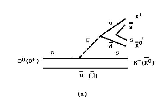
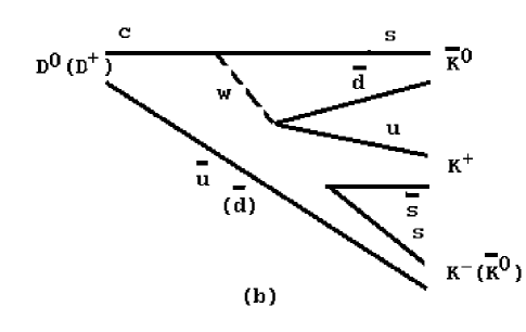
Figure 1:

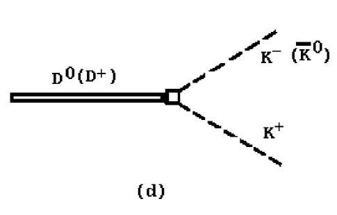
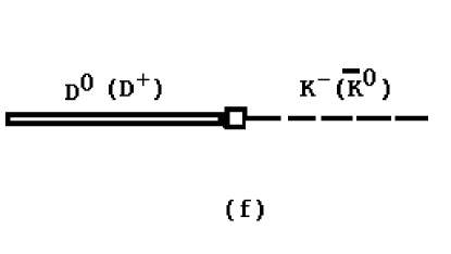
Figure 2:

References

• [1] For a review, see M. Wirbel, Prog. in Part. and Nucl. Phys. 21, 33 (1989);
A. J. Buras and M. K. Harlander, in Heavy Flavors, Eds. A.J. Buras, M. Lindner, World Scientific, 1992.
• [2] R. Ammar et al. (CLEO Collaboration), Phys. Rev. D44, 3383 (1991);
P. L. Fradetti et al. (E687 Collaboration), Phys. Lett. B286, 195 (1992).
• [3] M. B. Wise, Phys. Rev. D45, 2188 (1992). For a review, see M. B. Wise, Lectures given at the CCAST Symposium on Particle Physics at the Fermi Scale (1993), preprint CALT-68-1860.
• [4] T.-M. Yan, H.-Y. Cheng, G.-L. Lin, Y.C. Lin and H.-L. Yu, Phys. Rev. D46, 1148 (1992).
• [5] G. Burdman and J. Donoghue, Phys. Lett. B280, 287 (1992);
P. Cho, Phys. Lett. B285, 145 (1992).
• [6] L.-L. Chau and H.-Y. Cheng, Phys. Rev. D41, 1510 (1990).
• [7] F.J. Botella, S. Noguera and J. Portoles, Phys.Lett.B360, 101 (1995).
• [8] N. Isgur and M. Wise, Phys. Lett. B232, 113 (1989); B237, 527 (1990);
E. Eichten and B. Hill, Phys.Lett. B234, 511 (1990);
B. Grinstein, Nucl.Phys.B339, 253 (1990);
H. Georgi, Phys. Lett. B240, 447 (1990).
• [9] A. Manohar and H. Georgi, Nucl. Phys. B234, 189 (1984);
H. Georgi and L. Randall, Nucl. Phys. B276, 241 (1984);
H. Georgi, Phys. Lett. B298, 187 (1993).
• [10] H.-Y. Cheng, C.-Y. Cheung, G.-L. Lin, Y.C. Lin, T.-M. Yan and H.-L. Yu, Phys.Rev.D49, 2490 (1994);
N. Kitazawa and T. Kurimoto, Phys.Lett.B323, 65 (1994);
N. Di Bartolomeo, R. Gatto, F. Feruglio and G. Nardulli, Phys.Lett.B347, 405 (1995).
• [11] S. Barlag et al. (ACCMOR Collaboration), Phys. Lett. B278, 480 (1992).
• [12] S. Weinberg, Physica 96A, 327 (1979);
J. Gasser and H. Leutwyler, Ann. Phys. (NY) 158, 142 (1984).
See also the books Howard Georgi, ”Weak Interactions and Modern Particle Theory” (Benjamin/Cummings, 1984), and John F. Donoghue, Eugene Golowich, Barry R. Holstein, ”Dynamics of the Standard Model” (Cambridge Univ. Press, 1992).
• [13] M. Bauer, B. Stech and M. Wirbel, Z.Phys.C34, 103 (1987).
• [14] J. Gasser and H. Leutwyler, Ann. of Phys. 158, 142 (1984); Nucl. Phys. B 250, 465 (1985);
J. L. Goity, Phys. Rev. D 46, 3929 (1992);
D. Du, C. Liu and D.-X. Zhang, Phys. Lett. B317, 179 (1993).
• [15] Particle Data Group, Phys. Rev. D50, 3$-I$ (1994).
Table