We study the sensitivity of the processes $e^{+}e^{-}\to\ell\bar{\nu}_{\ell}\;q\bar{q}^{\prime}$ at LEP2 energies on the non-standard trilinear gauge couplings (TGC), using the optimal observables method. All relevant leading logarithmic corrections to the tree-order cross section, as well as experimental resolution effects have been studied. Taking into account correlations among the different TGC parameters we show that the limits on the TGC can reach the level of 0.15 (1sd) at 161 GeV with 100 pb^-1, a challenge for the first LEP2 phase. At higher energies this can be improved drastically, reaching the level of 0.02 (1sd).

DEMO-HEP-96/01
May 1996

One of the two most important measurements at LEP2 energies will be the determination of the trilinear vector boson couplings [1, 2, 3, 4], a characteristic manifestation of the underlying non-Abelian symmetry of elementary particle interactions [5].

In order to study the trilinear boson couplings we need a parametrization of these interactions that goes beyond the Standard Model . There are, of course, several possibilities to accomplish this task, but we are going to restrict ourselves to the most economical one by considering C$-$ and P$-$ conserving interactions. The relevant interaction Lagrangian is usually written in the following form [2]:

$${\cal L}_{TGC} = \sum_{V=\gamma,Z}e\>g_{V}\left(V_{\mu}W^{-\mu\nu}W^{+}_{\nu}-V_{\mu}W^{+\mu\nu}W^{-}_{\nu}+\kappa_{V}V_{\mu\nu}W^{+\mu}W^{-\nu}\right)$$ (1)

$$+ e\>{\lambda_{\gamma}\over M_{W}^{2}}A_{\mu\rho}W^{+\rho\nu}W^{-\mu}_{\nu}+e\>\mbox{ctg~{}}\theta_{w}{\lambda_{Z}\over M_{W}^{2}}Z_{\mu\rho}W^{+\rho\nu}W^{-\mu}_{\nu}$$

where

$$V_{\mu\nu}=\partial_{\mu}V_{\nu}-\partial_{\nu}V_{\mu},\;\;W^{\pm}_{\mu\nu}=\partial_{\mu}W^{\pm}_{\nu}-\partial_{\nu}W^{\pm}_{\mu}\;\;.$$

$W^{\pm}$ is the $W$-boson field, and $g_{\gamma}=1$, $g_{Z}=\mbox{ctg~{}}\theta_{w}$, $\kappa_{\gamma}=\kappa_{Z}=1$ and $\lambda_{\gamma}=\lambda_{Z}=0$ at tree order in the Standard Model . It is more convenient to express the different couplings in terms of their deviations from the Standard Model values. For this we define the following deviation parameters[2]:

$$\delta_{Z}=g_{Z}-\mbox{ctg~{}}\theta_{w}\;\;\;\;x_{\gamma}=\kappa_{\gamma}-1\;\;\;\;x_{Z}=(\kappa_{Z}-1)(\mbox{ctg~{}}\theta_{w}+\delta_{Z})\;.$$ (2)

It is worth while to note that the interaction Lagrangian becomes linear with respect to the above parameters (including also $\lambda_{\gamma}$ and $\lambda_{Z}$).

During the last years, considerable progress has been achieved concerning the understanding of the physics underlying the non-standard boson self-couplings. As Gounaris and Renard [6] showed, the deviations from the Standard Model couplings can be parametrized in a manifestly gauge-invariant (but still non-renormalizable) way, by considering gauge-invariant operators involving higher-dimensional interactions among gauge bosons and Higgs field. These operators will be scaled by an unknown parameter $\Lambda_{NP}$, which might be understood as the characteristic scale of New Physics effects. In order to describe all five C$-$ and P$-$ conserving couplings introduced in Eq.(1) we need operators with dimension up to eight. On the other hand restricting ourselves to $SU(2)_{L}\times U(1)_{Y}$-invariant operators with dimension up to six, which are the lowest order ones in $1/\Lambda_{NP}$ expansion, we can have the following list [7]:

$${\cal O}_{B\Phi} = B^{\mu\nu}(D_{\mu}\Phi)^{\dagger}(D_{\nu}\Phi)$$

$${\cal O}_{W\Phi} = (D_{\mu}\Phi)^{\dagger}\;\mbox{\boldmath$\tau$}\cdot\mbox{\boldmath$W$}^{\mu\nu}(D_{\nu}\Phi)$$

$${\cal O}_{W} = {1\over 3!}(\mbox{\boldmath$W$}^{\mu}_{\;\rho}\times\mbox{\boldmath$W$}^{\rho}_{\;\nu})\cdot\mbox{\boldmath$W$}^{\nu}_{\;\mu}$$ (3)

where $\tau_{i}={1\over 2}\sigma_{i}$ ($\sigma_{i}$ are the Pauli matrices),

$$B_{\mu\nu}=\partial_{\mu}B_{\nu}-\partial_{\nu}B_{\mu}$$

where $B_{\mu}$ is the $U(1)_{Y}$ gauge field,

$$\mbox{\boldmath$W$}_{\mu\nu}=\partial_{\mu}\mbox{\boldmath$W$}_{\nu}-\partial_{\nu}\mbox{\boldmath$W$}_{\mu}-g\mbox{\boldmath$W$}_{\mu}\times\mbox{\boldmath$W$}_{\nu}$$

where $W$ are the $SU(2)_{L}$ gauge fields and

$$\Phi=\left(\begin{array}[]{c}\phi^{+}\\ {1\over\sqrt{2}}(v+H+i\phi^{0})\end{array}\right)$$ (6)

is the Higgs doublet. The covariant derivative $D_{\mu}$ is given, as usual, by

$$D_{\mu}=\partial_{\mu}+i\;g\mbox{\boldmath$\tau$}\cdot\mbox{\boldmath$W$}_{\mu}-i\;g^{\prime}B_{\mu}$$

and $e=g\sin\theta_{w}=g^{\prime}\cos\theta_{w}$.

The interaction Lagrangian can be written now as

$${\cal L}_{TGC}=i\,g^{\prime}{a_{B\Phi}\over m_{W}^{2}}{\cal O}_{B\Phi}+i\,g{a_{W\Phi}\over m_{W}^{2}}{\cal O}_{W\Phi}+g{a_{W}\over m_{W}^{2}}{\cal O}_{W}$$ (7)

where the relations between $a_{W\Phi}$, $a_{B\Phi}$, $a_{W}$ and the deviation parameters of Eq.(2) are given by:

$$\delta_{Z}=a_{W\Phi}/\left(\sin\theta_{w}\cos\theta_{w}\right)\;\;\;\;x_{\gamma}=a_{B\Phi}+a_{W\Phi}\;\;\;\;\lambda_{\gamma}=a_{W}$$

$$x_{Z}=-\tan\theta_{w}x_{\gamma}\;\;\;\;\lambda_{Z}=\lambda_{\gamma}$$ (8)

In order to study the effect of TGC, one traditionally considered the reaction $e^{+}e^{-}\to W^{+}W^{-}$, taking into account the subsequent decay of the $W$’s in a four-fermion final state. These final states can be classified in three categories, namely the ‘leptonic’ $\ell_{1}\bar{\nu}_{\ell_{1}}\ell_{2}^{*}\nu_{\ell_{2}}$, the ‘semileptonic’ $\ell\bar{\nu}_{\ell}\;q\bar{q}^{\prime}$ and the hadronic $q_{1}\bar{q}^{\prime}_{1}\bar{q}_{2}q^{\prime}_{2}$ ($q$ and $q^{\prime}$ refer to up- and down-type quarks respectively). Semileptonic seems to be the most favoured channel [8] for studying TGC, since it contains the maximum kinematical information, taking into account that charge-flavour identification in four jet channel is rather inefficient and the cross section for the leptonic mode is suppressed. It is the goal of the present paper to study the effect of TGC, in their three parameter version Eq.(7), in the processes

$$e^{+}e^{-}\to\ell\bar{\nu}_{\ell}\;q\bar{q}^{\prime}$$ (9)

where $\ell$ is an electron or a muon, at LEP2 energies, based on the four-fermion Monte Carlo generator ERATO[9, 10, 11]. The final state $\tau\bar{\nu}_{\tau}\;q\bar{q}^{\prime}$ will not be considered here due to the special difficulties to identify $\tau$’s in this environment.

Figure 1: Single-resonant graph where TGC are contributing.

From the point of view of the four-fermion production, $e^{+}e^{-}\to W^{+}W^{-}$ calculations are equivalent to the narrow width approximation, $\Gamma_{W}\to 0$, which requires that both $W$’s are kinematically allowed to be on-shell. This last requirement implies of course that the overall energy should be above the $2m_{W}$ threshold and therefore it is not adequate for the first phase of LEP2, where $\sqrt{s}=161$ GeV. Moreover in $e^{+}e^{-}\to W^{+}W^{-}$ the invariant masses of the produced fermion pairs, $\ell\bar{\nu}_{\ell}$ and $q\bar{q}^{\prime}$, are identical to the $W$ mass, which requires experimental selection algorithms, whose efficiency is some times questionable, and more importantly their interplay with TGC studies can not be estimated, unless a full four-fermion calculation is used. On the other hand there are nowadays widely available four-fermion calculations[9, 12, 10] where TGC are included beyond the narrow width approximation. This enable us to study TGC not only in the double-resonant (CC3) graphs contributing to $e^{+}e^{-}\to W^{+}W^{-}$ but also in the single-resonant ones shown in Fig.1, which moreover become dominant at very high energies.

In the actual calculations presented in this paper we have used the ERATO Monte-Carlo generator. A detailed description of ERATO can be found in references [9, 10, 11]. The basic ingredients of the calculation are the following:

1. Exact tree-order matrix elements for the processes $e^{+}e^{-}\to\ell\bar{\nu}_{\ell}\;q\bar{q}^{\prime}$, based on helicity amplitude calculations [7, 9], including all TGC interactions described by Eq.(1).

2. Phase-space generation algorithm based on a multi-channel Monte Carlo approach, including weight optimization[13].

3. Treatment of unstable particle ($W$ and $Z$) width consistent with gauge-invariance and high-energy unitarity [9, 14, 15].

4. Initial state radiation (ISR) based on the structure function approach[16, 10], including soft-photon exponentiation as well as leading logarithmic (LL) contributions up to order $O(\alpha^{2})$.

5. Coulomb correction to the double resonant (CC3) graphs [16].

Moreover in order to avoid matrix element singularities as well as to be as close as possible to the experimental situation, the ‘canonical cuts’ of reference [10] have been applied:

$$175^{o}\geq\theta_{\ell}\;,\;\theta_{jet}\geq 5^{o},\;\;\;E_{\ell}\geq 1\mbox{ GeV}\;,\;\;E_{jet}\geq 3\mbox{ GeV}\;\;\mbox{and}\;\;m_{q,\bar{q}^{\prime}}\geq 5\mbox{ GeV}$$ (10)

The input Standard Model parameters we have used are as follows:

$$M_{W}=80.23\mbox{ GeV},\;\;\Gamma_{W}=2.033\mbox{ GeV},\;\;M_{Z}=91.188\mbox{ GeV},\;\;\Gamma_{Z}=2.4974\mbox{ GeV},$$

$$\sin^{2}\theta_{w}=0.23103\;\;\mbox{and}\;\;\alpha=1/128.07$$ (11)

As far as the ISR structure function is concerned the value $\alpha=1/137.036$ is used.

Most of the techniques used up to now to determine the sensitivity of a given reaction on the TGC have been based on a Maximum-Likelihood fit to Monte-Carlo generated four-fermion data. In its most advanced version [17], which is capable of dealing with low statistics data without any binning procedure, one maximizes the log-likelihood function:

$$\ln{\cal L}_{ML}=\sum_{i}\ln p(\Omega_{i},\vec{a})\;\;,$$ (12)

where the sum is running over the event sample. $\Omega_{i}$ represents the collection of the independent kinematical variables describing the i-th event, $\vec{a}=(a_{W\Phi},a_{B\Phi},a_{W})$ is the vector whose components are the three TGC parameters, $p(\Omega_{i},\vec{a})$ is the probability to find an event at such a phase space point, and is defined by:

$$p(\Omega,\vec{a})={1\over\sigma}{d\sigma\over d\Omega}$$ (13)

with

$$\sigma=\int_{V}{d\sigma\over d\Omega}d\Omega\;\;.$$

Although this is the most direct method to analyse experimental data, one has to calculate the full differential cross section for a large number of TGC parameter values, which is rather time-consuming.

On the other hand, since the interaction Lagrangian is linear with respect to TGC, one can easily write the differential cross section in the form

$${d\sigma\over d\Omega}=c_{0}(\Omega)+\sum_{i}a_{i}c_{1,i}(\Omega)+\sum_{i,j}a_{i}a_{j}c_{2,ij}(\Omega)$$ (14)

and of course in a similar way the total cross section is written as

$$\sigma=\hat{c}_{0}+\sum_{i}a_{i}\hat{c}_{1,i}+\sum_{i,j}a_{i}a_{j}\hat{c}_{2,ij}$$ (15)

where hatted $c$’s are integrals of unhatted ones over the phase space. It is now straightforward to verify that the probability has an expansion

$$p(\Omega,\vec{a})=p_{0}(\Omega)\left\{1+\sum_{i}a_{i}\left({c_{1,i}(\Omega)\over c_{0}(\Omega)}-{\hat{c}_{1,i}\over\hat{c}_{0}}\right)+\mbox{higher orders}\right\}$$ (16)

where

$$p_{0}(\Omega)={1\over\sigma}{d\sigma\over d\Omega}\bigg{|}_{\vec{a}=0}$$ (17)

is the Standard Model distribution.

Assuming now that the data are well described by the Standard Model ($\vec{a}=0$) distribution it is easy to calculate the so-called information matrix [18], which determines the sensitivity of the fit on the parameters $\vec{a}$, and is defined by:

$$I_{ij} \equiv E\bigg{[}\left({\partial\over\partial a_{i}}\ln{\cal L}_{ML}\right)\left({\partial\over\partial a_{j}}\ln{\cal L}_{ML}\right)\bigg{]}$$

$$= -E\bigg{[}{\partial\over\partial a_{i}}{\partial\over\partial a_{j}}\ln{\cal L}_{ML}\bigg{]}$$

where

$$E[A]=\int\prod_{i=1}^{N}\{d\Omega_{i}\;p_{0}(\Omega_{i})\}A(\Omega_{1},...,\Omega_{N})$$ (19)

represents the mean value of a function $A$. To the lowest order one has that $I_{ij}=N{\cal B}_{ij}$ where

$${\cal B}_{ij}\equiv\langle{c_{1,i}\over c_{0}}{c_{1,j}\over c_{0}}\rangle{{}_{{}_{{0}}}}-\langle{c_{1,i}\over c_{0}}\rangle{{}_{{}_{{0}}}}\langle{c_{1,j}\over c_{0}}\rangle{{}_{{}_{{0}}}}$$ (20)

and

$$\langle A\rangle{{}_{{}_{{0}}}}=\int d{\Omega}\;p_{0}(\Omega)\;A(\Omega)\;\;.$$ (21)

Using now Eq.(16) one has that the set of the phase-space functions:

$${\cal O}_{i}={c_{1,i}(\Omega)\over c_{0}(\Omega)}\;\;,$$ (22)

are the optimal observables[19], whose mean values and covariance matrix will determine the sensitivity on the TGC parameters, and it is equivalent, to the lowest order, to the log-likelihood method. More specifically we have that

$$\langle{\cal O}_{i}\rangle=\langle{\cal O}_{i}\rangle{{}_{{}_{{0}}}}+\sum_{j}a_{j}{\cal B}_{ij}.$$

The estimator is now given by

$$\bar{a}_{i}=\sum_{j}{\cal B}^{-1}_{ij}\left(\langle{\cal O}_{j}\rangle-\langle{\cal O}_{j}\rangle{{}_{{}_{{0}}}}\right)$$

and the corresponding covariance matrix

$$V(\bar{a})={1\over N}\;\;{\cal B}^{-1}\cdot V({\cal O})\cdot{\cal B}^{-1}$$

where $V({\cal O})$ is the covariance matrix of the ${\cal O}_{i}$ defined by

$$V({\cal O})_{ij}=\langle{\cal O}_{i}{\cal O}_{j}\rangle-\langle{\cal O}_{i}\rangle\langle{\cal O}_{j}\rangle$$

which in the ideal case, where measured distributions are identical to the Standard Model predictions, is given by $V({\cal O})={\cal B}$.

One-dimensional investigations assuming that all but one of the $a$’s are non-vanishing, result in parameter errors (1sd) given by

$$\delta a_{i}={1\over\sqrt{N{\cal B}_{ii}}}\;\;.$$ (23)

On the other hand taking into account the correlations one has to diagonalize the covariance matrix $V(\bar{a})$ and therefore

$$\delta a^{D}_{i}={1\over\sqrt{N\lambda_{i}}}$$ (24)

where $\lambda_{i}$ are the eigenvalues of the matrix ${\cal B}$ and the parameters $a^{D}_{i}$ are defined by

$$a^{D}_{i}=\vec{e}_{i}\cdot\vec{a}\;\;.$$ (25)

where $\vec{e}_{i}$ are the corresponding eigenvectors of ${\cal B}$.

In all calculations presented in this paper, $N$ is taken to be the predicted number of events in the Standard Model , defined as

$$N=4\;L\;\sigma$$

where $\sigma$ is the corresponding total cross section, $L$ is the integrated luminosity and the factor $4$ takes into account the four equivalent channels (all described by the same matrix elements), i.e. $e^{+}e^{-}\to\ell\bar{\nu}_{\ell}\;q\bar{q}^{\prime}$ stands for $e^{+}e^{-}\to$, $\ell\bar{\nu}_{\ell}\;u\bar{d}$, $\ell\bar{\nu}_{\ell}\;c\bar{s}$, $\ell^{*}{\nu}_{\ell}\;d\bar{u}$ and $\ell^{*}{\nu}_{\ell}\;s\bar{c}$.

At this point it is worth to emphasize that expanding the log-likelihood function to higher orders in $a_{i}$ will allow us to identify observables which probe the behaviour of $\log{\cal L}_{ML}$ up to the corresponding order. Therefore there is no limitation, in principle, to establish a one-to-one mapping between Maximum-Likelihood and optimal observables. On the other hand one can argue that since we have truncated our interaction lagrangian to the order $1/\Lambda_{NP}^{2}$, consistency would require that each observable should also be trusted up to this order and therefore only linear terms should be kept. In any case optimal observable and Maximum-Likelihood become identical in the high statistics limit, $N\to\infty$, and therefore we are well justified to use optimal observables to estimate the errors on TGC parameters. Moreover, the optimal observables method can easily be extended[19], when the variation of the total event rate is taken into account, corresponding to the so-called Extended Maximum Likelihood (EML) method. It should be noted, however, that in the case where some of the $c_{1,i}$ terms vanish, or $\langle({c_{1}\over c_{0}})^{2}\rangle-\langle{c_{1}\over c_{0}}\rangle^{2}\sim O(1/\sqrt{N})\times(\langle{c_{2}\over c_{0}}{c_{1}\over c_{0}}\rangle-\langle{c_{2}\over c_{0}}\rangle\langle{c_{1}\over c_{0}}\rangle),$ leading and next-to-leading terms become equally important and an analysis based on the optimal observables of Eq.(22) breaks down. Fortunately, such a ‘pathological’ case is not observed at LEP2 energies.

Finally, from the point of view of a weighted Monte-Carlo approach, which is frequently used in the phenomenological analyses, optimal observables offer a very efficient, fast and economic way to estimate the sensitivity of a given process on the TGC (or any kind of ‘deviation’ parameters). The only thing one has to do is to calculate the correlation matrix ${\cal B}_{ij}$. This should be contrasted with log-likelihood methods where either one has to repeat the calculation for a large set of TGC parameter values which adequately covers the parameter space, or to store information on the coefficients appearing in the Eq.(14) for each generated ‘event’. Of course from the point of view of ‘unweighted’ or real data analysis these arguments do not apply any more, since now local (event-by-event) information is any way available. In this case log-likelihood would be preferable over optimal observables, since it is not restricted to the linear terms.

$\sqrt{s}$	161	176	190	205
$e$	$\begin{array}[]{c}\mbox{\tt{0.456 0.180 0.087}}\\ \mbox{\tt{0.180 0.173 0.008}}\\ \mbox{\tt{0.087 0.008 0.117}}\end{array}$	$\begin{array}[]{c}\mbox{\tt{0.587 0.086 0.238}}\\ \mbox{\tt{0.086 0.087 0.014}}\\ \mbox{\tt{0.238 0.014 0.311}}\end{array}$	$\begin{array}[]{c}\mbox{\tt{0.973 0.115 0.420}}\\ \mbox{\tt{0.115 0.135 0.024}}\\ \mbox{\tt{0.420 0.024 0.605}}\end{array}$	$\begin{array}[]{c}\mbox{\tt{1.400 0.163 0.601}}\\ \mbox{\tt{0.163 0.209 0.036}}\\ \mbox{\tt{0.601 0.036 0.969}}\end{array}$
	124.6(6)	489(2)	591(2)	621(2)
$\mu$	$\begin{array}[]{c}\mbox{\tt{0.271 0.013 0.092}}\\ \mbox{\tt{0.013 0.019 0.004}}\\ \mbox{\tt{0.092 0.004 0.093}}\end{array}$	$\begin{array}[]{c}\mbox{\tt{0.547 0.033 0.253}}\\ \mbox{\tt{0.033 0.037 0.014}}\\ \mbox{\tt{0.253 0.014 0.313}}\end{array}$	$\begin{array}[]{c}\mbox{\tt{0.956 0.063 0.447}}\\ \mbox{\tt{0.063 0.084 0.028}}\\ \mbox{\tt{0.447 0.028 0.620}}\end{array}$	$\begin{array}[]{c}\mbox{\tt{1.435 0.111 0.660}}\\ \mbox{\tt{0.111 0.151 0.044}}\\ \mbox{\tt{0.660 0.044 1.036}}\end{array}$
	123.1(5)	476(2)	567(2)	585(2)

Table 1: The correlation matrix for $e$ and $\mu$ channels at LEP2 energies for TGC parameters $\vec{a}=(a_{W\Phi},a_{B\Phi},a_{W})$. Also shown are the cross sections as well as their Monte Carlo errors in femtobarns.

In table 1 we present the results for the correlation matrix, ${\cal B}_{ij}$, for centre of mass energies 161, 176, 190 and 205 GeV. The total cross sections are also presented. As is evident from this table, the correlation between the different $a$’s are rather strong, which suggests that an analysis taking into account these correlation is indispensable. As is easily seen from this table, the correlations are much stronger between $a_{W\Phi}$ and $a_{W}$ as compared with $a_{B\Phi}$, which in general gives the smallest contribution.

An other very interesting result, is that electron and muon channels exhibit different behaviour depending on the energy. The difference is more prominent at the threshold region, $\sqrt{s}$=161Gev. This is due to the contribution from single-resonant $W$-production graph Fig.1, which becomes relatively more important at threshold. On the other hand at higher energies, the dominance of the double-resonant graphs (CC3) restores universality among electrons and muons, and the correlation matrix is almost identical for both channels. It is worth to emphasize that differences in the correlation matrix ($\sim 100\%$) among $e$ and $\mu$ channels are much more important than the differences in the total cross section ($\sim 1\%$), reflecting the fact that the graph of Fig.1 contributes mainly to the shape of the differential cross section rather than to its overall normalization.

$\sqrt{s}$	$e$	$\mu$
161	$\begin{array}[]{cc}0.559&\left(\mbox{\tt{0.889, 0.419, 0.183}}\right)\\ 0.125&\left(\mbox{\tt{0.128,-0.613, 0.779}}\right)\\ 0.062&\left(\mbox{\tt{0.438,-0.670,-0.599}}\right)\\ \end{array}$	$\begin{array}[]{cc}0.311&\left(\mbox{\tt{0.920, 0.046,-0.390}}\right)\\ 0.054&\left(\mbox{\tt{0.388, 0.039, 0.921}}\right)\\ 0.018&\left(\mbox{\tt{0.058,-0.998,-0.018}}\right)\\ \end{array}$
176	$\begin{array}[]{cc}0.734&\left(\mbox{\tt{0.863, 0.125, 0.489}}\right)\\ 0.183&\left(\mbox{\tt{0.443, 0.274,-0.853}}\right)\\ 0.068&\left(\mbox{\tt{0.241,-0.953,-0.181}}\right)\\ \end{array}$	$\begin{array}[]{cc}0.711&\left(\mbox{\tt{0.841, 0.052, 0.537}}\right)\\ 0.152&\left(\mbox{\tt{0.535, 0.051,-0.843}}\right)\\ 0.035&\left(\mbox{\tt{0.072,-0.997,-0.015}}\right)\\ \end{array}$
190	$\begin{array}[]{cc}1.258&\left(\mbox{\tt{0.835, 0.097, 0.540}}\right)\\ 0.339&\left(\mbox{\tt{0.517, 0.193,-0.833}}\right)\\ 0.116&\left(\mbox{\tt{0.186,-0.976,-0.111}}\right)\\ \end{array}$	$\begin{array}[]{cc}1.269&\left(\mbox{\tt{0.821, 0.057, 0.568}}\right)\\ 0.311&\left(\mbox{\tt{0.565, 0.055,-0.823}}\right)\\ 0.080&\left(\mbox{\tt{0.078,-0.997,-0.013}}\right)\\ \end{array}$
205	$\begin{array}[]{cc}1.838&\left(\mbox{\tt{0.817, 0.094, 0.569}}\right)\\ 0.557&\left(\mbox{\tt{0.549, 0.173,-0.817}}\right)\\ 0.183&\left(\mbox{\tt{0.175,-0.980,-0.089}}\right)\\ \end{array}$	$\begin{array}[]{cc}1.932&\left(\mbox{\tt{0.802, 0.065, 0.594}}\right)\\ 0.548&\left(\mbox{\tt{0.589, 0.075,-0.804}}\right)\\ 0.141&\left(\mbox{\tt{0.097,-0.995,-0.023}}\right)\\ \end{array}$

Table 2: The eigenvalues and the corresponding eigenvectors of the correlation matrices given in table 1.

In table 2 we show the eigenvalues of the correlation matrix, as well as the corresponding eigenvectors. These eigenvectors define directions in the three-parameter space, which are uncorrelated and therefore parameter errors can be safely extracted. As we can see the two dominant eigenvalues correspond to directions in the three-parameter space related predominantly to $a_{W\Phi}$ and $a_{W}$, whereas the lowest eigenvalue is always related to $a_{B\Phi}$. This $a_{B\Phi}$ suppression is due to the fact that in the double resonant (CC3) graphs relative cancellations between terms proportional to $x_{\gamma}$ and $x_{Z}$ take place. An exception to this pattern is due to the electron channel at 161 GeV, where the mixing is much more important, reflecting the contribution from the graph of Fig.1. This is easily understood, since in the amplitude corresponding to this graph the relative cancellations between $x_{\gamma}$ and $x_{Z}$ are now destroyed due to the the presence of the $t$-channel photon propagator, which means that the $t$-channel single-resonant graph receives contributions only from $x_{\gamma}$ and $\lambda_{\gamma}$ whereas contributions from $x_{Z}$, $\delta_{Z}$ and $\lambda_{Z}$ are suppressed.

Finally in table 3 one-standard-deviation errors are presented by combining $e$ and $\mu$ in the following way

$${\cal B}_{ij}={\cal B}^{(e)}_{ij}{\sigma^{(e)}\over\sigma^{(e)}+\sigma^{(\mu)}}+{\cal B}^{(\mu)}_{ij}{\sigma^{(\mu)}\over\sigma^{(e)}+\sigma^{(\mu)}}\;\;.$$

and

$$N=4L(\sigma^{(e)}+\sigma^{(\mu)})\;\;.$$

In all our studies, $L$ is taken to be 100 pb^-1 at 161 GeV and 500 pb^-1 at all higher LEP2 energies. In $1d$-case, corresponding to ‘one-dimensional log-likelihood fit’, errors on $a_{W\Phi}$, $a_{W}$, $a_{B\Phi}$ are shown. For $3d$-cases, the errors correspond to the linear combinations defined in Eq.(25). Nevertheless in table 3 we kept the notation of $a_{W\Phi}$, $a_{W}$ and $a_{B\Phi}$ for $3d$-cases, since the corresponding eigenvector, $a_{W\Phi}^{D}$ for instance, is mainly composed by $a_{W\Phi}$ and so on for the other TGC parameters. It is rather evident that correlations, though important, do not alter dramatically the estimate of the errors based on simple ‘one-dimensional’ investigations, and therefore $1d$ limits are still useful.

	$a_{W\Phi}$ $a_{W}$ $a_{B\Phi}$	$a_{W\Phi}$ $a_{W}$ $a_{B\Phi}$	$a_{W\Phi}$ $a_{W}$ $a_{B\Phi}$	$a_{W\Phi}$ $a_{W}$ $a_{B\Phi}$
$\sqrt{s}$	161	176	190	205
$1d$	0.16 0.31 0.32	0.030 0.041 0.091	0.021 0.026 0.062	0.017 0.020 0.048
$3d$	0.15 0.32 0.44	0.027 0.056 0.098	0.018 0.036 0.066	0.015 0.027 0.050
$3d^{\prime}$	0.18 0.37 0.50	0.031 0.064 0.110	0.021 0.041 0.073	0.017 0.030 0.055

Table 3: One standard deviation errors on TGC parameters. $1d$ means that the correlation matrix is assumed diagonal where for $3d$ and $3d^{\prime}$ all correlations have been taken into account. Finally in $3d^{\prime}$ ‘resolution’ effects are also included as described in the text.

In real life, detector resolution effects and reconstruction algorithm, tend to distort the ‘observed’ distributions as compared with the ‘theoretical’ predictions. This can in principle, mimic the effects of TGC, and therefore should be studied on a generator level. This study requires a good knowledge of the specific detector and should be carried out in detail by our expiremental colleagues. Nevertheless, we can estimate the order of magnitude of these effects based on the following very general assumption, that the distorted-‘observed’ distribution $p_{eff}$ is expressed as a convolution integral given by:

$$p_{eff}(\Omega_{meas},\vec{a})=\int p(\Omega_{true},\vec{a})\;\;S(\Omega_{true},\Omega_{meas})\;\;d\Omega_{true}$$ (26)

where $p(\Omega_{true},\vec{a})$ is the theoretically predicted distribution and $S(\Omega_{true},\Omega_{meas})$ is a ‘resolution’ function, giving the probability that an event ‘measured’ at phase space point $\Omega_{meas}$ is coming from a ‘true’ event at a phase space point $\Omega_{true}$.

In order to simulate in a simple way the ‘resolution’ function we have implemented the following algorithm:

• To each generated event we calculate the nine kinematical variables, in the lab frame, $E_{i},\theta_{i},\phi_{i}$, $i=1,2,3$, which correspond to the ‘visible’ particles, namely the lepton $\ell$ and the two jets $q,\bar{q}^{\prime}$.

• To each of the above variables we assign a new one,

  $$\theta\to\theta^{\prime},\;\;\phi\to\phi^{\prime}\;\;\mbox{and}\;\;E\to E^{\prime}$$

  following the rule that primed variables are normally distributed around the original ones with variances given by:

  $$\sigma_{E_{\ell}}=0.03\;E_{\ell},\;\sigma_{\theta_{\ell}}=0.0002,\;\sigma_{\phi_{\ell}}=0.0002,\;$$

  $$\sigma_{E_{jet}}=0.15\;E_{jet},\;\sigma_{\theta_{jet}}=0.03,\;\sigma_{\phi_{jet}}=0.04\;.$$

• Then, this artificially generated phase space point is subjected to a ‘kinematical constraint fit’ algorithm, by including a ‘missing energy’ (neutrino) four-momentum in such a away that

  $$\sum_{i=1}^{4}E_{i}=2\;E_{beam}\;\;\;\mbox{and}\;\;\;\sum_{i=1}^{4}\vec{p}_{i}=0$$

  This is achieved by a local (event by event) rescaling of the energies of the two jets, which are expected to be the worst measured quantities. This rescaling is defined by the minimization of the following $\chi^{2}$ function:

  $$\chi^{2}=\sum_{jets}{\left(E_{i}^{\prime}-E_{i}\right)^{2}\over\sigma^{2}_{i}\;}.$$

  Note that, although the original phase space point is generated taking into account initial state radiation, in the ‘reconstructed’ one we have artificially neglected it and the total energy is normalized to the overall constant beam energy.

• Finally the usual cuts of Eq.(10) are applied, including now a special cut on the missing $p/_{T}$ vector, $p/_{T}\geq 15\mbox{ GeV}$. This supplementary cut is applied in order to minimize the background coming from the process $e^{+}e^{-}\to e^{+}e^{-}\;q\bar{q}$, where the $e^{+}$ is assumed to be lost into the beam, which leads to the same final state $e^{-}+2\mbox{jets}$. Using ERATO we have checked that the reconstructed $p/_{T}$ in the background process is well below 15 GeV, whereas the $p/_{T}$ distribution of our ‘signal’ processes $e^{+}e^{-}\to\ell\bar{\nu}_{\ell}\;q\bar{q}$ has a negligible tail below 15 GeV.

Using now the kinematical information from the above algorithm we can calculate the new correlation matrix, $\tilde{{\cal B}}_{ij}$, using Eq.(26), and from it the new information matrix given by

$$I^{new}=I\cdot\tilde{I}^{-1}\cdot I$$

The 1sd-erros on TGC parameters calculated through $I^{new}$ are given in table 3, under the $3d^{\prime}$-case. Comparing with the $3d$ case, we see that the effect is of the order of 10-20% on the parameter errors, which is at an acceptable level. We have checked that reasonable input values for the variances $\sigma_{E}$, $\sigma_{\theta}$ and $\sigma_{\phi}$ give more or less the same results. The same is still true if we replace the polar representation of the observed momenta by the cartesian one. This means that resolution effects are unlikely to destroy the measurement of TGC. Moreover it is worth to emphasize that ‘unfolding’ techniques can also be used in order to minimize this effect, relying on a good knowledge of the detector as well as of the physics included in the event generator programme.

We conclude by summarizing the results of our study:

1. Sensitivities on TGC at LEP2 are of the level of 0.15-0.5 (1sd) at 161 GeV, making the threshold phase of LEP2 the best up to date world measurement of TGC. Higher energies will drastically improve these limits, almost by an order of magnitude, reaching the level of 0.02. Taking into account information from other channels, such as the four-jet one, further improvement is expected.

2. The electron channel due to single-resonant $W$ contributions is rather important at 161 GeV and special studies are needed on the experimental side, in order to maximize selection efficiencies in this channel. Finite-width, ISR and Coulomb corrections are also indispensable at 161 GeV.

3. Resolution effects are unlikely to drastically alter this picture, leading to a mild loosening of the sensitivity limits by a 10-20% factor.

As a postscript of our study we present in Fig.2 the distributions of the optimal observable ${\cal O}_{a_{W\Phi}}$ at 161GeV. The solid line corresponds to the ideal case, where the measured distribution is assumed to be identical with the predicted one, whereas the dashed line is calculated by the convolution integral Eq.(26), based on our naive ‘resolution’ model. Also shown are the two-dimensional scatter plots, between the generated and ‘measured’ values of ${\cal O}_{a_{W\Phi}}$. Although our ‘resolution’ model is very simplistic, it suggests that optimal observables can be used in the experimental analysis of four-fermion data. Optimal observables are the ‘phase-space’ variables exhibiting the maximum sensitivity on TGC and therefore they effectively reduce the number of independent phase-space variables from eight to three, which is rather appreciable from the experimental point of view. On the other hand their sensitivity on ‘resolution’ effects seems to be rather mild. Nevertheless their usefulness has to be verified by a detailed analysis at the experimental level.

Acknowledgements
It is pleasure to thank H. Phillips, R.Sekulin and S.Tzamarias for making the simulation values of the experimental resolutions available to the author. This work is supported in part by the EU grant CHRX-CT93-0319.

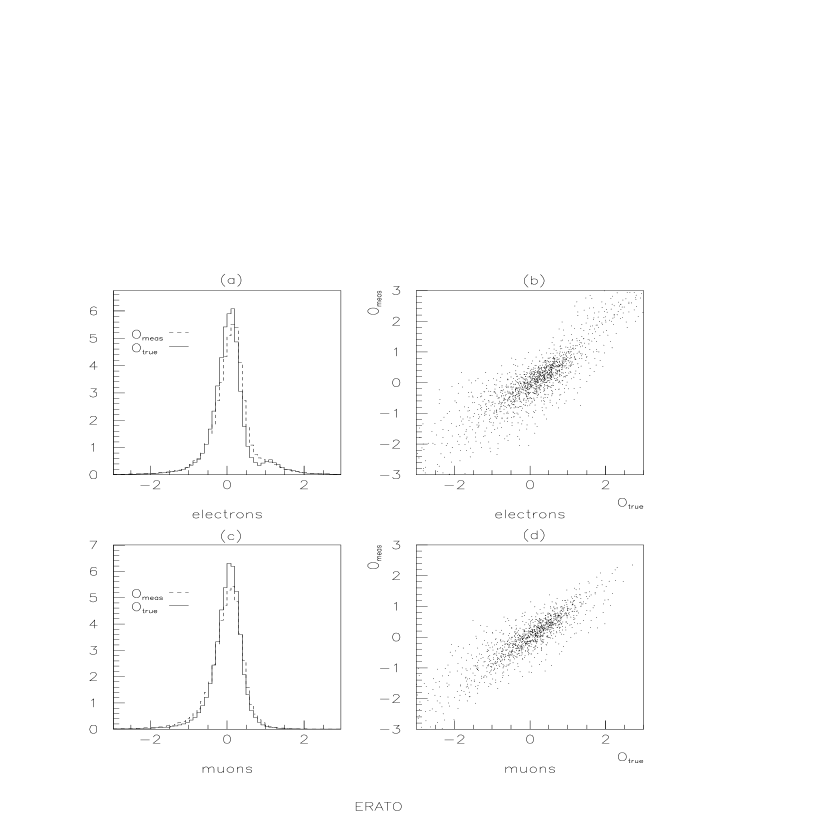
Figure 2: The distribution of the optimal observable corresponding to the parameter $a_{W\Phi}$ at 161 GeV, for electron (a) and muon (c) channels. Also shown are the scatter plots (b) and (d).

References

- [1] K. Gaemers and G. Gounaris, Z.Phys. C1(1979) 259.
- [2] M. Bilenky et al., Nucl. Phys. B409 (1993) 22.
- [3] K. Hagiwara, R. Peccei, D. Zeppenfeld and K. Hikasa, Nucl.Phys. 282 (1987) 253.
- [4] E.N. Argyres and C.G. Papadopoulos, Phys. Lett. B263 (1991) 298.
-
[5]
S.L.Glashow, Nucl.Phys. 22 (1961) 579;
S.Weinberg, Phys.Rev.Lett. 19 (1967) 1264;
A.Salam, in Elementary particle theory, ed. N.Svartholm (Almquist and Wiksell, Stockholm, 1968)p.367 - [6] G.J. Gounaris and F.M. Renard, Z.Phys. C59 (1993) 133.
- [7] C.G. Papadopoulos, Phys. Lett. B333 (1994) 202.
- [8] G. Gounaris et al., ‘Triple gauge boson couplings’ in Physics at LEP2, ed. G. Altarelli et al., Vol.1, p. 525, CERN 96-01, February 1996 & hep-ph/9601233.
- [9] C.G. Papadopoulos, Phys. Lett. B352 (1995) 144.
- [10] D. Bardin et al., ‘Event generators for physics’ in Physics at LEP2, ed. G. Altarelli et al., Vol.2, p. 3, CERN 96-01, February 1996.
- [11] Write-up in preparation
- [12] F.A. Berends and A. van Sighem, Nucl. Phys. B454 (1995) 467.
- [13] R.Kleiss and R.Pittau, Comp.Phys.Commun. 83 (1994) 141.
- [14] U. Baur and D. Zeppenfeld, Phys.Rev.Lett. 75 (1995) 1002.
- [15] E.N. Argyres et al, Phys.Lett. B358 (1995) 339
- [16] W. Beenakker et al., ‘ cross sections and distributions’ in Physics at LEP2, ed. G. Altarelli et al., Vol.1, p. 79, CERN 96-01, February 1996 & hep-ph/9602351.
- [17] R. L. Sekulin, Phys.Lett. B338 (1994) 369.
- [18] W.T. Eadie et al., Statistical Methods in Experimental Physics, North-Holland, Amsterdam, 1971.
- [19] M. Diehl and O. Nachtmann, Z.Phys. C 62 (1994) 397.