CU-TP-746

Cavendish-HEP-96/04

hep-ph/9605302

May 1996

Large multiplicity fluctuations and saturation effects in onium collisions

A.H. Mueller

Department of Physics, Columbia University,

New York, NY 10027, USA

G.P. Salam

Cavendish Laboratory, Cambridge University,

Madingley Road, Cambridge CB3 0HE, UK

e-mail: salam@hep.phy.cam.ac.uk

This paper studies two related questions in high energy onium-onium scattering: the probability of producing an unusually large number of particles in a collision, where it is found that the cross section for producing a central multiplicity proportional to $k$ should decrease exponentially in $\sqrt{k}$. Secondly, the nature of gluon (dipole) evolution when dipole densities become so high that saturation effects due to dipole-dipole interactions become important: measures of saturation are developed to help understand when saturation becomes important, and further information is obtained by exploiting changes of frame, which interchange unitarity and saturation corrections.

1 Introduction

The Balitsky, Fadin, Kuraev and Lipatov (BFKL) equation [1, 2, 3] is meant to describe the energy dependence of certain high energy hard processes. For the BFKL equation to be applicable certain conditions must be met: (i) The process, or part of a process, to be described should have only a single hard transverse momentum scale. Processes having more than one hard scale may have significant contribution from the Dokshitzer, Gribov, Lipatov, Altarelli and Parisi (DGLAP) equation [4, 5, 6] which governs scale dependence in QCD. Certain observables (e.g. [7]) are known to satisfy this criterion though they have not yet been well measured. (ii) The rapidity of the hard process, related to the centre of mass energy $E$ and the hard transverse momentum scale $k$ by $Y=\ln E^{2}/k^{2}$, should be large. The BFKL equation includes all terms $(\alpha_{s}Y)^{n}$ in the coupling but neglects factors of $\alpha_{s}$ not accompanied by factors of $Y$. There is a vigorous effort [8] to systematically include the first non-leading terms, an $\alpha_{s}$ unaccompanied by a $Y$ and this should improve the accuracy and reliability of the BFKL equation.

The BFKL equation should describe high energy processes having a single hard scale in a limited range of rapidity. When $Y$ becomes too large, unitarity corrections become important and slow the rate of growth with energy. At even higher values of energy one expects parton densities to become so large that the whole perturbative QCD picture breaks down leading to a new regime of weak coupling but high density non-perturbative QCD. The goal in small-x physics is to understand, experimentally and theoretically, the onset of BFKL behaviour, its modification due to unitarity corrections as one proceeds to higher energies and finally the nature of the transition to the high density (saturation) regime at even higher energies.

From a theoretical point of view the simplest process to study is high energy heavy quarkonium-heavy quarkonium scattering. If the onium is sufficiently heavy the radius of the onium is small enough to set the single hard scale of the process. Any understanding of BFKL dynamics and beyond gained in studying heavy onium collisions should be applicable to the more experimentally accessible single hard scale processes mentioned above. In the large $N_{c}$ limit of QCD a dipole picture of high energy heavy onium-heavy onium scattering has been developed which is equivalent to the usual BFKL description [9, 10, 11, 12, 13]. In this dipole picture the light-cone wave function of a heavy onium is viewed as a collection of colour dipoles. The dipoles are made up of the quark part of a gluon (or the heavy quark itself) and the antiquark part of a different gluon (or the heavy antiquark). High energy elastic scattering in the BFKL approximation proceeds by two-gluon exchange between a right-moving dipole in the right-moving onium and a left-moving dipole in the left-moving onium.

Perhaps the main advantage of the dipole picture is that the equation governing the number and distribution of dipoles in the light-cone wave function of the onium is a branching equation which allows Monte Carlo methods to be used. In a recent paper [14], one of us has studied high energy onium-onium scattering from energies where the BFKL approximation is valid into the higher energy regime where unitarity limits, for a fixed impact parameter of the scattering, are reached. In the centre of mass system unitarity corrections are simply the independent scattering of two or more dipoles of the right-moving onium with two or more dipoles of the left-moving onium. Because of the large number of (small) dipoles in an onium wave function unitarity corrections become important when the dipoles are relatively dilute in the onium so that independent multiple scatterings are the natural leading corrections to the BFKL approximation.

The purpose of the present paper is to study two related questions, the probability of producing an unusually large number of particles in an onium-onium collision and the nature of gluon (dipole) evolution when dipole densities become so dense that saturation effects due to dipole-dipole interactions become important. At a given energy dipole densities in an onium wave function are largest not in a typical configuration but rather in rare high multiplicity fluctuations. Thus attempts to measure saturation will naturally focus on the high multiplicity tail of particle production.

One cannot directly study particle production in the dipole formalism. In the dipole picture the $t=0$ light-cone wave function is constructed. This is sufficient to describe an elastic scattering, but it is not sufficient to describe an inelastic event where one must follow the time evolution of the wave function to a large positive time when particles (or jets) are produced. However, using the Abramovskii, Gribov, Kancheli (AGK) cutting rules [15] one can relate particle production and forward elastic scattering involving one or more dipole scatterings. While there has been no detailed proof of the AGK rules in QCD it is likely that they are correct and we assume that this is the case in the present paper.

We calculate $\sigma_{k}$ the cross section for $k$ cut pomerons when $k$ takes values far above average. The multiplicity of produced particles, in the central unit of rapidity, should be proportional to $k$. We begin by studying a toy model which obeys dipole evolution but where the absence of transverse dimensions makes analytic solutions to the multiplicity distribution possible. Our main result for the toy model is given in eq. (9) where $\sigma_{k}$ is seen to decrease exponentially in ${\sqrt{k}}$ at large $k$, a tail much longer than that given by KNO scaling [16]. We have not been able to solve the large $k$ behaviour for the $k$ cut pomeron contribution to a zero impact parameter collision in QCD, $\mathrm{d}\sigma_{k}/\mathrm{d}^{2}\mathbf{r}(\mathbf{r}\simeq 0)$. However, Monte Carlo results obtained using OEDIPUS (Onium Evolution, Dipole Interaction and Perturbative Unitarisation Software) [17] indicate a very similar $k$-dependence to that found in the toy model with an $e^{-A{\sqrt{k+n}}}$ dependence at large $k$. The same dependence, but with different values of $A$ and $n$, also well describes onium-onium collisions integrated over impact parameter. The fact that the high multiplicity tail extends so far encourages one to believe that high parton density systems can be produced at reasonable accelerator energies if the right signal is found to trigger on the interesting physics associated with saturation.

In section 3, we turn to a study of saturation [18], beginning with defining measures of saturation. Saturation effects show up as a modification of the simple branching picture of dipoles in constructing the square of the onium wave function. Thus, a non-independence of the dipoles in an onium wave function is a measure of saturation. However, it is not known how to estimate the interaction of dipoles in an onium wave function directly. One expects that the interaction of a slightly right-moving dipole with higher rapidity right-moving dipoles in a right-moving onium should be similar to that of a slightly left-moving dipole with the right-moving onium. This latter interaction is just the scattering amplitude for a simple dipole with an onium state and is straightforward to calculate. Thus one measure of saturation of a light-cone onium wave function is the interaction probability with an opposite moving elementary dipole. This measure of saturation is however time consuming to evaluate. A more efficient measure is the overlap that a given dipole in the onium wave function has with all the other dipoles in the wave function. Happily, it turns out that these two measures are strongly correlated so that the simpler overlap measure can be used.

The toy model discussed earlier also furnishes a useful model of saturation. Saturation is expected to slow the growth of the number of dipoles. By comparing the cross section calculated in frames where the two incoming particles share the incoming energy differently, a consistency condition, requiring that the cross section be frame independent, gives sufficient information to determine dipole branching as a function of rapidity. While at low energy the rate of parton evolution grows exponentially in rapidity, as in BFKL evolution, that rate reaches a constant (saturates) at high rapidity as shown in eq. (16).

The toy model can be used to study the intriguing, and still not well understood, relationship between unitarity limits and saturation. In QCD the centre of mass onium-onium scattering, at a fixed impact parameter, reaches the unitarity limit at energies well below that at which saturation effects begin to appear. However, if onium-onium scattering is viewed in a frame where, say, the left-moving onium has a small rapidity, the scattering looks exactly like the measure we have earlier discussed for saturation since now the left-moving onium is simply a single dipole. Thus the multiple scatterings in the centre of mass system must show up as saturation effects in a system where one of the onia carries almost all the energy. This can be most sharply seen in the toy model by considering a toy onium scattering on a toy nucleus consisting of $N$ onia. Here it is found that saturation effects found earlier are exactly what is necessary to make onium-nucleus scattering the same in either the frame where the onium is at rest or in the frame where the nucleus is at rest.

In QCD it is not possible to do such complete analytical calculations, however, we have found a phenomenological modification of dipole branching eq. (33) which makes onium-onium and onium-nucleus scattering reasonably frame independent. One particularly sharp way to see the necessity of saturation effects and their frame dependence is to compare the S-matrix, at zero impact parameter, for onium-onium scattering in the centre of mass frame with that obtained in a laboratory frame at very high rapidities. At rapidities large enough so that the S-matrix has become very small the evaluation of the S-matrix neglecting saturation is determined by the very low multiplicity fluctuations of the wave function. We find, on theoretical grounds and from numerical simulations, that $S\sim e^{-c(Y-Y_{0})^{2}}$. However, without saturation effects $c$ is a factor of 2 larger in the lab frame than in the centre of mass. Saturation effects will slow the growth of dipoles in the laboratory frame so that the typical wave function configuration agrees with the centre of mass calculation coming from rare fluctuations. This is exactly what happens in the toy model as can be seen by comparing eqs. (26) and (28).

At large impact parameters, $r$, we find that the property of the centre of mass frame, that saturation corrections set in much later than unitarity effects, starts to break down. This is brought about by several factors. At large $r$, the amplitude has a significant contribution from asymmetric onium-onium configurations, for example where one onium has a only central dense cluster of small dipoles (of order of the onium size): for there to be an interaction the second onium must have small dipoles at the relevant large impact parameter, where they are likely to be much more dilute. This kind of scattering looks similar to a lab frame collision, and hence the saturation and unitarity corrections will be similar. A second point is that one might expect a distribution of large dipoles which looks relatively dilute, to have only small saturation corrections. However, the sequence of evolution to produce this distribution will often have passed through a stage with a dense collection of small dipoles, whose evolution would be significantly altered by saturation effects, reducing the production of large dipoles in the first place. Overall, in the centre of mass frame, at large impact parameters, these effects combine to give saturation corrections of the same order as the unitarity corrections. Fortunately, the total scattering cross section is not too strongly affected by these large impact parameters, and it is still reasonable to neglect saturation effects in its calculation.

2 Cuts

2.1 The AGK cutting rules

It is most useful to start from the AGK cutting rules [15] as expressed in [19]. The cross section, $\sigma_{k}$ involving the exchange of exactly $k$ cut pomerons can be expressed as follows:

$$\sigma_{k}=\sum_{\nu=k}^{\infty}(-1)^{\nu-k}2^{\nu}C^{\nu}_{k}F^{(\nu)},$$ (1)

where $F^{(\nu)}$ is the amplitude for the exchange of $\nu$ pomerons. In this notation, the total cross section $\sigma_{t}$ is

$$\sigma_{t}=2\sum_{\nu=1}^{\infty}(-1)^{\nu-1}F^{(\nu)}.$$ (2)

One knows from previous work [11, 14] that the terms of the sum in eq. (2) diverge as a factorial, and therefore so will the terms in eq. (1). The reason for this divergence is that rare configurations of the onia contribute increasingly large amounts to the amplitudes for higher pomeron exchange. The solution is to sum multiple pomeron amplitudes before averaging over onium configurations. Applying this method here one obtains the differential cross section for obtaining $k$ cut pomerons. The $\nu$ pomeron amplitude for a fixed impact parameter $\mathbf{r}$ between the two onia (of sizes $\mathbf{b}$ and $\mathbf{b}^{\prime}$, evolved to rapidities $y$ and $Y-y$) is:

$$F^{(\nu)}(\mathbf{r},\mathbf{b},\mathbf{b}^{\prime},Y,y)=\frac{1}{\nu!}\sum_{\gamma,\gamma^{\prime}}P_{\gamma}(\mathbf{r}_{0},\mathbf{b},y)P_{\gamma^{\prime}}(\mathbf{r}_{0}+\mathbf{r},\mathbf{b}^{\prime},Y-y)(f_{\gamma,\gamma^{\prime}})^{\nu},$$ (3)

where $f_{\gamma,\gamma^{\prime}}$ is the two gluon exchange interaction amplitude between a pair of configurations $\gamma$ and $\gamma^{\prime}$ which occur with probabilities $P_{\gamma}(\mathbf{r}_{0},\mathbf{b},y)$ and $P_{\gamma^{\prime}}(\mathbf{r}_{0}+\mathbf{r},\mathbf{b}^{\prime},Y-y)$ from onia situated at $\mathbf{r}_{0}$ and $\mathbf{r}_{0}+\mathbf{r}$. Substituting this into eq. (1) gives

$$\frac{\mathrm{d}^{2}\sigma_{k}}{\mathrm{d}^{2}\mathbf{r}}=\frac{1}{k!}\sum_{\gamma,\gamma^{\prime}}P_{\gamma}(\mathbf{r}_{0},\mathbf{b},y)P_{\gamma^{\prime}}(\mathbf{r}_{0}+\mathbf{r},\mathbf{b}^{\prime},Y-y)(2f_{\gamma,\gamma^{\prime}})^{k}\exp(-2f_{\gamma,\gamma^{\prime}}).$$ (4)

The cross section for obtaining no cuts is the difference between the unitarised cross section and $\sum_{k=1}^{\infty}\sigma_{k}$, which comes out as:

$$\frac{\mathrm{d}^{2}\sigma_{0}}{\mathrm{d}^{2}\mathbf{r}}=\sum_{\gamma,\gamma^{\prime}}P_{\gamma}(\mathbf{r}_{0},\mathbf{b},y)P_{\gamma^{\prime}}(\mathbf{r}_{0}+\mathbf{r},\mathbf{b}^{\prime},Y-y)\left(1-\mathrm{e}^{-f_{\gamma,\gamma^{\prime}}}\right)^{2}.$$ (5)

In the work that follows, $y$ will be set to $Y/2$, so that we will be examining the number of cuts at a central rapidity.

2.2 Toy model calculation

As was the case for the unitarised amplitude [11], the evaluation of eq. (4) is very difficult to do analytically, because it requires a detailed understanding of the distribution of dipole configurations for an onium. However some of the features of multiple cut cross sections can be extracted by examining a “toy” model which has no transverse dimensions [11].

The main feature of the toy model is that the probability of obtaining a large number $n$ of dipoles has an exponential distribution, $P_{n}\simeq e^{-n/\mu}/\mu$, where $\mu$ is the mean number of dipoles (proportional to $e^{(\alpha_{\mathcal{P}}-1)y}$ for an onium evolved to a rapidity $y$). One can show that in the case with transverse dimensions, the probability of obtaining a large density of dipoles also has a distribution which is an exponential in the density [14]. It is this similarity which leads to the correspondence between the toy model and the case with two transverse dimensions. In the toy model, the cross section for an interaction with $k$ cut pomerons is

$$\sigma_{k}=\frac{1}{k!}\sum_{m,n}(2f\alpha_{S}^{2}nm)^{k}\exp(-2f\alpha_{S}^{2}nm)P_{m}P_{n},$$ (6)

where the interaction amplitude between two dipoles is defined to be $f\alpha_{S}^{2}$ (equivalent to $f_{\gamma,\gamma^{\prime}}$ above). There are two limits which can be taken. Let $F^{(1)}$ be the amplitude for exchange of one pomeron. If $kF^{(1)}=kf\alpha_{S}^{2}\mu^{2}\ll 1$, then unitarisation effects (the exponential factor) are unimportant, and the evaluation of the cuts cross sections is very similar to the evaluation of the multiple pomeron amplitudes [11]:

$$\sigma_{k}\simeq k!(2F^{(1)})^{k}\mathrm{e}^{-2k^{2}F^{(1)}}.$$ (7)

The opposite limit is when unitarisation effects are important, $kF^{(1)}=kf\alpha_{S}^{2}\mu^{2}\gg 1$ (and also $k/F^{(1)}\gg 1$). Approximating the sums by integrals, and changing variables to $n=\sqrt{u}\mathrm{e}^{\xi}$ and $m=\sqrt{u}\mathrm{e}^{-\xi}$ gives

$$\sigma_{k}\simeq\frac{1}{\mu^{2}k!}(2f\alpha_{S}^{2})^{k}\int\mathrm{d}u\mathrm{d}\xi u^{k}\mathrm{e}^{-2f\alpha_{S}^{2}u}\mathrm{e}^{-2(\cosh\xi)\sqrt{u}/\mu}.$$ (8)

Performing the $\xi$ integration using the saddle point approximation, it is clear that the integral is dominated by a region where $m$ and $n$ are similar. Performing the second integration gives

$$\sigma_{k}\simeq\frac{1}{2F^{(1)}}\left(\frac{2F^{(1)}\pi^{2}}{k}\right)^{1/4}\exp\left(-\sqrt{\frac{2k}{F^{(1)}}}\right).$$ (9)

The unusual feature of this result is the square root dependence on $k$ in the exponential. Given that the number of cuts is related to the final state multiplicity, one might have expected the usual KNO type [16] exponential distribution. The origin of the $\sqrt{k}$ behaviour is that, in the region of configuration space contributing to the $k$-cut amplitude, the factor $(2f\alpha_{S}^{2}nm)^{k}\exp(-2f\alpha_{S}^{2}nm)$ is the most rapidly varying and fixes the dominant values of $n,m\propto\sqrt{k}$. The probabilities associated with the relevant configurations just fix the normalisation, with $P(\sqrt{k})\sim\mathrm{e}^{-\sqrt{k}}$.

2.3 Monte Carlo results for differential cut cross sections

One is most likely to find a similarity between the toy model results and the realistic situation, by examining the differential cut cross sections, which eliminates two of the transverse degrees of freedom. In [14] correspondence between the toy model and Monte Carlo results for zero impact parameter has already been established for the multiple pomeron exchange amplitudes. The main difference was that where the quantity $\nu$ occurred in an expression relating to $\nu$-pomeron exchange, it had to be replaced with $(\nu+n)$ where $n$ was a constant which originated from the details of the dynamics in the transverse dimensions. One might expect a similar effect when looking at cut cross sections, and one can examine the differential cross section for small impact parameters for behaviour of the form

$$\frac{\mathrm{d}^{2}\sigma_{k}}{\mathrm{d}^{2}\mathbf{r}}(r\simeq 0)\simeq\exp[-A(k+n)^{\gamma}+B]$$ (10)

where $A$, $B$, $n$ and $\gamma$ are constants to be determined. The first stage is to ensure that one really does have $\gamma=1/2$. By defining $l_{k}=-\ln\mathrm{d}^{2}\sigma_{k}/\mathrm{d}^{2}\mathbf{r}$ and plotting

$$\Gamma_{k}=\frac{l_{k+1}-l_{k-1}}{2l_{k}-l_{k-1}-l_{k+1}}=\frac{2(k+n)}{1-\gamma}+O(1/(k+n))$$ (11)

Figure 1: The upper plot shows $\Gamma_{k}$ for fixed impact parameter: a test that the cut cross sections show the behaviour corresponding to eq. (10) (actually averaged over a range of $r=0\to 0.6b$); the lower plot shows the multiple cut cross sections together with a fit of the form eq. (10) (for the range $r=0.2b\to 0.3b$).

(essentially the ratio of first and second derivatives) one can eliminate $A$ and $B$. Figure 1 shows this quantity as a function of $k$, determined using the OEDIPUS Monte Carlo simulation [17]. For $k$ sufficiently large, the linear behaviour is very clear, and the slope corresponds to $\gamma=1/2$. The value of the intercept with the $k$ axis yields $n$, which has a value of $10$. This is somewhat larger than the corresponding value found for multiple pomeron exchange ($\nu\to\nu+n$, with $n\sim 3$). The difference can be explained by arguing that the multiple pomeron and multiple cut cross sections are sensitive to the dipole distributions (and the manner in which they differ from an exponential) in different ways.

The other property to examine is the variation of $A$ with $Y$. One clearly cannot expect $A$ to be exactly $\sqrt{2/F^{(1)}(0)}$, however it might be reasonable for it to be proportional to $\sqrt{2/F^{(1)}(0)}$. Table 1 gives $A$ for two values of $Y$, indicating that to within the accuracy of the Monte Carlo results, this proportionality does hold.

$Y$	$n$	$A$	$F^{(1)}(0)$	$A/\sqrt{2/F^{(1)}(0)}$
10	7	4.45	0.436	2.08
14	10	2.21	1.62	1.99

Table 1: Parameterisations of cut distributions at central impact parameters.

The dependence of the distributions on $n$ is relatively weak which is why it is not determined more accurately. Table 1 therefore confirms that for the zero impact parameter cross section the distribution scales as suggested by the toy model.

2.4 Monte Carlo results for the integrated cut cross sections

One can argue that events with $k$ cut pomerons will have a multiplicity proportional to $k$. In an experimental situation, one might be able to determine the cross sections for various ranges of multiplicities, but this will correspond to cut cross sections integrated over impact parameter, for which there will not necessarily be any correspondence with the toy model. However figure 2 shows that a fit of the form eq. (10)

Figure 2: The upper plot shows $\Gamma_{k}$ for the integrated cross sections; the lower plot shows the multiple cut cross sections together with a fit of the form eq. (10).

$$\sigma_{k}\simeq\exp[-A(k+n)^{\gamma}+B]$$ (12)

works remarkably well. The value of $n$ turns out to be considerably smaller than for eq. (10): this is associated with the fact that at larger values of $r$ the value of $n$ decreases.

It is not clear why the $\exp(-A\sqrt{k+n})$ behaviour also applies to the integrated cross section. The results do however suggest that the variation of the coefficient $A$ with the rapidity is not as simple as in the toy model (or in the fixed impact parameter case). The numerical results for the variation with rapidity of the fraction of the cross section coming from different numbers of cuts is shown in figure 3.

Figure 3: The fraction of the total cross section coming from different numbers of cuts (indicated by the labels next to the curves) as a function of rapidity.

2.5 Spatial distribution of cut cross sections

Just as high numbers of pomeron exchange tend to be dominated by small impact parameters, one can expect events with large numbers of cuts also to be relatively central, because they are dominated by dense configurations, which arise most commonly at small impact parameters. This is illustrated in figure 4, which shows $\sigma_{k}(r>R)/\sigma_{k}$, the fraction of the $k$-cut cross section which comes from impact parameters larger than $R$, for various numbers of cuts, as a function of $R$.

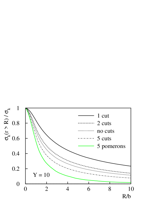
Figure 4: The fraction of the multiple cut cross section which comes from impact parameters larger than $R$ for a variety of numbers of cuts. At this rapidity, the mean number of cuts is $\sim 1.3$

One sees for example that about half the one-cut cross section is coming from a region $r<3.2b$, whereas the first half of the 5-cut cross section comes from $r<1.4b$. There is of course a limit to how central the many cut cross section can become, since any cross section is bound to be spread out over a region at least the size of the onia. The no cut cross section is also quite central: like the many cut cross sections, it is particularly sensitive to dense configurations. Note that all these cross sections have significant tails at large $r$. This is to be contrasted with the 5-pomeron curve, where the tail dies off quickly: the difference arises because of the unitarity corrections that are associated with multi-cut cross sections but not multi-pomeron contributions, and which limit the relative contributions from very dense configurations.

3 Saturation

In the calculations performed to determine the unitarity corrections [11, 14], it has been assumed that saturation of the wave function can be neglected. The justification for doing this is that in a situation where both wave functions are evolved to $Y/2$, unitarisation corrections will set in when $\alpha_{S}^{2}e^{(\alpha_{\mathcal{P}}-1)Y}\sim 1$, while saturation corrections for a particular dipole will be of the order $\alpha_{S}^{2}e^{(\alpha_{\mathcal{P}}-1)Y/2}$. Two problems can arise with this argument. The first relates to the question of whether $\alpha_{S}$ is small enough. In the calculations presented here, $\alpha_{S}\sim 0.2$, so when unitarisation is important one might expect $\alpha_{S}^{2}e^{(\alpha_{\mathcal{P}}-1)Y/2}\sim 0.2$. Since the conditions for saturation can only be guessed to within a factor of order 1, one is potentially close to the onset of saturation corrections as well. Secondly, the argument is based on the principle that the mean dipole density will be a good gauge of the saturation corrections. However in the case of unitarisation corrections, it has been shown [14] that the use of mean interactions can be very misleading. In this section we will perform a more sophisticated analysis of the importance of saturation corrections, relative to unitarity corrections. We will also present work on understanding wavefunction evolution once saturation becomes a large effect.

3.1 Measures of saturation

It is first necessary to develop a measure of saturation. Two methods will be used here. Firstly one can probe a wave function with an (unevolved) onium. The two gluon exchange amplitude between the wave function and the onium indicates the local density dipoles of size similar to the onium and might be similar to the interaction that a dipole in the wave function would have with its neighbours. Since the dipole-dipole interaction has spikes wherever two sources overlap, one should average the interaction over a region of roughly the onium size. The choice of the size of the region over which to average is one of the main uncertainties with this method. It also has the disadvantage of being relatively slow, because one needs to determine dipole-dipole interactions at many points to determine the saturation over the whole extent of the wave function and if one wants the saturation associated with dipoles of different sizes, one must use probes of different sizes.

The second method is more arbitrary, but much faster to compute. Each dipole has an “overlap” associated with it. For each pair of dipoles within the onium wave function which are separated by less than a certain distance (which will be a function of the dipole sizes) the quantity $\alpha_{S}^{2}c_{<}^{2}/c_{>}^{2}$ is added to the overlap for each of the two dipoles (where the smaller dipole has size $c_{<}$ and the larger, size $c_{>}$). This function is loosely based on the fact that the total two-gluon interaction amplitude between a pair of dipoles (moving fast relative to each other) has the form $\alpha_{S}^{2}c_{<}^{2}/c_{>}^{2}(1+\ln c_{>}/c_{<})/2$ and that it is dominated by a region where the two dipoles are close in impact parameter. This method has the advantage that one obtains a value of the saturation for each dipole.

Figure 5: The probability of a given onium configuration lying in a certain $I_{max}$, $O_{max}$ bin, for $y=10$.

Comparing the two methods one finds that there is a good (linear) correlation between them, as can be seen in figure 5 which shows the frequency distribution for configurations with various values of $I_{max}$ (the maximum interaction with the probe) and $O_{max}$ (the maximum overlap). One can carry out other comparisons, in particular, considering the location in impact parameter of the maximum saturation, and one again finds that the two methods give very similar results. In addition, if one examines other values of rapidity, one finds that the factor relating $I_{max}$ and $O_{max}$ stays approximately the same.

3.2 Distribution of $I_{max}$

The degree of saturation is obviously just related to the density of dipoles. Therefore the distribution of $I_{max}$ should be related to the probability of obtaining large densities, which has been shown to be exponential [14], the slope of the exponential being proportional to the mean density of dipoles. Instead of searching the whole relevant region of impact parameter for the location of $I_{max}$, one finds the location of the dipole corresponding to $O_{max}$ and bases the search for $I_{max}$ around that point. The probe size is always the same as the onium size.

One finds, as expected, that $I_{max}$ also shows an exponential behaviour, with a slope varying in proportion to the local density of dipoles. One also finds that the maximum saturation is usually close to the original onium which is also unsurprising since that is where the evolution has the longest rapidity range to produce a large number of dipoles.

While these properties are of general interest, one of the main reason for studying saturation is to see whether it is likely to affect the onium-onium cross section. So one needs to know the typical values of $I_{max}$ and also the correlation between $I_{max}$ for a pair of onium configurations and the interaction cross section for that pair of configurations.

Figure 6: The probability distribution of the larger $I_{max}$ from a pair of onia (‘unweighted’ curve), and the fractions of cross sections coming from configuration pairs with particular values of $I_{max}$ (‘1-pomeron’ and ‘unitarised’ curves); $Y=12$.

The most appropriate value of rapidity to examine is $Y=12$, since this is the rapidity for which the mean 1-pomeron amplitude at $r=0$, $F^{(1)}(r=0)$, is equal to 1 (the unitarity bound). Consider first the ‘unweighted’ curve of figure 6: this corresponds to the probability distribution of $I_{max}$ in onium-onium collisions with a total rapidity $Y=12$. The rapidity for each onium is $y=Y/2=6$. $I_{max}$ is now defined to be the larger of the $I_{max}$ values for the two onium configurations. One sees that typical values of saturation are $0.1\to 0.3$. The exponential probability distribution for large saturation is relatively clear. More relevant though are the distributions weighted with the onium-onium cross section for each configuration pair: the weighted distributions correspond to the fraction of the cross section coming from configuration pairs with a certain $I_{max}$, and one sees that the typical saturation has increased to be in the range $0.2\to 0.45$. There are two main reasons why configuration pairs with larger cross sections are associated with larger saturation. Firstly if one of the onia has a high density of dipoles in some region, then the interaction of that region with a second onium will be enhanced. A second possibility, which we will consider in more detail later, is that configurations which lead to a large interaction (e.g. those with large dipoles) are most likely to be produced through branching sequences which pass through a high density stage.

There remains the problem of assessing the effect that this degree of saturation would have. One can assume that saturation will start to become important when $I_{max}\sim 1$, but this is a very approximate condition, being uncertain to within at least a factor of two. This factor of two is critical: if the condition for saturation is $I_{max}\sim 2$ then there will be no problem with saturation at $Y=12$, on the other hand if it is $I_{max}\sim 1/2$ then saturation could significantly alter the results at this rapidity. If saturation is important then one wants to know how it will affect the evolution: for example the saturation might be large in one region of impact parameter, but the bulk of the cross section might come from different regions, not affected by saturation. The next sections address these and other issues.

3.3 Saturation in the toy model

One approach to the problem is again from the toy model, using the condition that the scattering amplitude must be independent of the frame in which calculation is performed. Equivalently, it shouldn’t matter which of the two onia one chooses to evolve. Starting with a state containing $n$ dipoles, the rate of branching into a state containing $n+1$ dipoles is defined to be $R_{n}$, while the interaction between two states with $n$ and $m$ dipoles respectively is $F(n,m)$. If the evolution is partitioned such that for an increase $\delta Y$ in total rapidity, the onium with $n$ dipoles evolves by $\xi\delta Y$ and the one with $m$ dipoles evolves by $(1-\xi)\delta Y$, then the evolution of the amplitude $F$ will be

$$\frac{\mathrm{d}F}{\mathrm{d}Y}=\xi R_{n}\left[F(n+1,m)-F(n,m)\right]+(1-\xi)R_{m}\left[F(n,m+1)-F(n,m)\right]$$ (13)

In the case of one pomeron exchange, one has $R_{n}=(\alpha_{\mathcal{P}}-1)n$ and $F(n,m)=f\alpha_{S}^{2}nm$ (where $f$ sets the strength of the interaction), giving

$$\frac{\mathrm{d}F^{(1)}}{\mathrm{d}Y}=[\xi+(1-\xi)](\alpha_{\mathcal{P}}-1)f\alpha_{S}^{2}nm$$ (14)

which is clearly independent of $\xi$.

If for $F(n,m)$ one uses the form which includes unitarity corrections, $F(n,m)=[1-\exp(-f\alpha_{S}^{2}nm)]$, one obtains the following expression for the evolution of the interaction:

$$\frac{\mathrm{d}F^{s}}{\mathrm{d}Y}=\left[\xi R^{s}_{n}\left(1-\mathrm{e}^{-f\alpha_{S}^{2}m}\right)+(1-\xi)R^{s}_{m}\left(1-\mathrm{e}^{-f\alpha_{S}^{2}n}\right)\right]e^{-\alpha_{S}^{2}mn}$$ (15)

where the superscript $s$ indicates that saturation is being taken into account. The condition that the growth of the cross section be independent of $\xi$, as well as one’s knowledge of the branching rate for small $n$ (where saturation should be unimportant) leads to the following expression for the rate of branching:

$$R^{s}_{n}=\frac{(\alpha_{\mathcal{P}}-1)}{f\alpha_{S}^{2}}\left(1-\mathrm{e}^{-f\alpha_{S}^{2}n}\right).$$ (16)

Note that though the interaction with a second onium was used in the determination of this branching rate, the result is independent of the state of the second onium.

To see what effect saturation will have on the final probability distribution of dipoles, one can use the following arguments. First take the case without saturation, in the continuum limit for $n$. The probability distribution satisfies

$$\frac{\mathrm{d}P}{\mathrm{d}y}=-\frac{\mathrm{d}R_{n}P}{\mathrm{d}n}=-(\alpha_{\mathcal{P}}-1)\frac{\mathrm{d}nP}{\mathrm{d}n}.$$ (17)

Changing variables to $Q=nP$, $\zeta=(\alpha_{\mathcal{P}}-1)y$ and $\nu=\ln n$, one has

$$\frac{\mathrm{d}Q}{\mathrm{d}\zeta}=-\frac{\mathrm{d}Q}{\mathrm{d}\nu},$$ (18)

whose solution (from our knowledge that $P=\exp[-(\alpha_{\mathcal{P}}-1)y-n\exp(-(\alpha_{\mathcal{P}}-1)y)]$) is

$$Q=\exp\left(\nu-\zeta-\mathrm{e}^{\nu-\zeta}\right).$$ (19)

In the case with saturation one has

$$\frac{\mathrm{d}P^{s}}{\mathrm{d}y}=-\frac{\mathrm{d}R_{n}^{s}P^{s}}{\mathrm{d}n}=-\frac{(\alpha_{\mathcal{P}}-1)}{f\alpha_{S}^{2}}\frac{\mathrm{d}(1-\mathrm{e}^{-f\alpha_{S}^{2}n})P^{s}}{\mathrm{d}n}.$$ (20)

By an appropriate change of variables, $Q^{s}=(1-\mathrm{e}^{-f\alpha_{S}^{2}n})P^{s}/(f\alpha_{S}^{2})$, $\zeta=(\alpha_{\mathcal{P}}-1)y$ and $\nu^{s}=\ln[(\mathrm{e}^{f\alpha_{S}^{2}n}-1)/(f\alpha_{S}^{2})]$, one can obtain an equation identical to eq. (18)

$$\frac{\mathrm{d}Q^{s}}{\mathrm{d}\zeta}=-\frac{\mathrm{d}Q^{s}}{\mathrm{d}\nu^{s}}.$$ (21)

Because, in the limit of small $n$ and $\zeta$, $Q^{s}\simeq Q$ and $\nu^{s}\simeq\nu$, the equation for $Q^{s}$ will have the same initial conditions as that for $Q$ and therefore their solutions will be the same. Translating this back to the variables $P^{s}$ and $n$, one has

$$P^{s}(n,y)=\exp\left[f\alpha_{S}^{2}n-(\alpha_{\mathcal{P}}-1)y-\frac{1}{f\alpha_{S}^{2}}\left(\mathrm{e}^{f\alpha_{S}^{2}n}-1\right)\mathrm{e}^{-(\alpha_{\mathcal{P}}-1)y}\right].$$ (22)

For $\mathrm{e}^{(\alpha_{\mathcal{P}}-1)y},n\ll 1/(f\alpha_{S}^{2})$ this approximates to the solution without saturation. The main feature of this solution though is that at large $y$, instead of there being an exponential distribution in $n$ with mean $\exp((\alpha_{\mathcal{P}}-1)y)$, one now has a solution which has a maximum at

$$n=\frac{1}{f\alpha_{S}^{2}}\left[(\alpha_{\mathcal{P}}-1)y+\ln f\alpha_{S}^{2}\right],$$ (23)

and which dies off quickly beyond that.

One effect of this modified probability distribution is to increase the value of the $S$-matrix at very large rapidities. If one calculates the $S$-matrix in a centre of mass frame (rapidity $Y$ divided equally between the two onia) neglecting saturation one obtains [11]:

$$S(Y)\simeq\frac{-1}{f\alpha_{S}^{2}\mathrm{e}^{(\alpha_{\mathcal{P}}-1)Y}}\ln\left[f\alpha_{S}^{2}\left(1+\frac{1}{f\alpha_{S}^{2}\mathrm{e}^{(\alpha_{\mathcal{P}}-1)Y/2}}\right)^{2}\right].$$ (24)

Note that this is much larger than the value of the $S$-matrix that one obtains from typical configurations (namely $\exp(-f\alpha_{S}^{2}e^{(\alpha_{\mathcal{P}}-1)Y})$). This difference arises because the $S$-matrix is dominated by a small fraction of configurations which have few dipoles.

Calculating the $S$-matrix including saturation (done in the lab frame, to reduce sensitivity to the use of the continuum limit, though the result is of course independent of frame), one obtains

$$S(Y)\simeq\frac{1}{f\alpha_{S}^{2}\mathrm{e}^{(\alpha_{\mathcal{P}}-1)Y}}\left[\ln f\alpha_{S}^{2}\mathrm{e}^{(\alpha_{\mathcal{P}}-1)Y}\right].$$ (25)

When $f\alpha_{S}^{2}\mathrm{e}^{(\alpha_{\mathcal{P}}-1)Y/2}\ll 1$, eqs. (24) and (25) give the same result, consistent with the idea that saturation should not be important in the centre of mass frame for that energy range. However for $f\alpha_{S}^{2}\mathrm{e}^{(\alpha_{\mathcal{P}}-1)Y/2}\gg 1$, eqs. (24) and (25) do differ (the saturated case has a logarithmic dependence on energy, absent from the calculation without saturation), because saturation then matters in the evolution of the onium wave functions, even in the centre of mass frame.

While this approach works well for the toy model, in the real case, an analogous method will turn out to be too complex to be useful. Nevertheless one can also make use of the effect of a change of frame on the average (unitarised) amplitude. The simplest pair of frames to examine would be centre of mass and lab frames for onium-onium scattering. However one finds that, except for logarithmic factors, the $S$-matrix behaves in a very similar way in the two. Consider instead collisions between a toy onium and a toy “nucleus” consisting of $N$ onia. Two frames will be used: a lab frame $L_{O}$ where the onium is at rest, and a lab frame $L_{N}$ where the nucleus is at rest. At high energies (neglecting saturation), in frame $L_{N}$, with the onium being evolved, the matrix is approximately

$$S_{N}\simeq\frac{1}{Nf\alpha_{S}^{2}\mathrm{e}^{(\alpha_{\mathcal{P}}-1)Y}}.$$ (26)

Except for logarithmic terms (and the factor $N$) this has the same leading energy behaviour as the centre of mass onium-onium $S$-matrix, and is similarly dominated by those rare configurations of the onium which have few dipoles (the common configurations have such a large number of dipoles that their contribution to the $S$-matrix can be neglected).

In the $L_{O}$ frame, it is the nucleus which it is evolved. Assuming for the sake of the argument that the constituent onia evolve independently (consistent with our neglect of saturation), configurations with few dipoles will be much rarer, because they require that none of the $N$ constituent onia should have evolved much. Accordingly, when one calculates the $S$-matrix, one finds

$$S_{O}\simeq\frac{1}{\left(f\alpha_{S}^{2}\mathrm{e}^{(\alpha_{\mathcal{P}}-1)Y}\right)^{N}},$$ (27)

which is much smaller than the result in the $L_{N}$ frame. One way of restoring the correspondence is by requiring that saturation alter the probability distribution of the number of dipoles so that the value of the $S$-matrix for a typical configuration of the nucleus is now

$$S_{O}^{\mathrm{typical}}\sim\frac{1}{Nf\alpha_{S}^{2}\mathrm{e}^{(\alpha_{\mathcal{P}}-1)Y}}.$$ (28)

Equivalently the typical number of dipoles must be of the order of $[(\alpha_{\mathcal{P}}-1)Y+\ln Nf\alpha_{S}^{2}]/(f\alpha_{S}^{2})$. Note that this is just the result of eq. (23) (except for the $\ln N$ term which is a result of the use of nuclei). The advantage of examining the effect of frame changes on the average $S$-matrix is that one can transfer the arguments fairly straightforwardly to the case of scattering with transverse dimensions.

3.4 Saturation in the case with transverse dimensions

The real case, including transverse dimensions, is very much more complicated, to a large extent because the dipole picture breaks down at high dipole densities and one needs to take into account quadrupoles, hexapoles, and other more complicated colour structures [12, 20]. This section will deal with various approaches that one can nevertheless try in order to deduce more information about the effects of saturation in the real case, still using the requirement of frame independence.

It is simple to write down the equation which must be satisfied for frame independence to hold. This will be the equivalent (with transverse dimensions) of the independence of eqs. (13) and (15) on $\xi$. Let $\gamma$ be a particular gluon configuration and $\{\gamma_{\mathbf{b}}\}$ be the set of all colour configurations with an extra gluon added at transverse position $\mathbf{b}$, with $\gamma_{\mathbf{b}}$ being any particular one of these. In the dipole approximation (large $N_{c}$), a particular $\gamma_{\mathbf{b}}$ corresponds to the gluon having originated from a particular dipole. Define also $F_{\gamma,\gamma^{\prime}}(\mathbf{r})$ to be the interaction between configurations $\gamma$ and $\gamma^{\prime}$ (moving in opposite directions) when they have a relative separation in impact parameter of $\mathbf{r}$. Then for the scattering to be frame independent (or equivalently for it not to matter which onium is evolved) the rate of evolution $R(\gamma\to\gamma_{\mathbf{b}})$ must satisfy

$$\sum_{\{\gamma_{\mathbf{b}}\}}\int\mathrm{d}^{2}\mathbf{b}R(\gamma\to\gamma_{\mathbf{b}})\left(F_{\gamma_{\mathbf{b}},\gamma^{\prime}}-F_{\gamma,\gamma^{\prime}}\right)=\sum_{\{\gamma_{\mathbf{b}}^{\prime}\}}\int\mathrm{d}^{2}\mathbf{b}R(\gamma^{\prime}\to\gamma_{\mathbf{b}}^{\prime})\left(F_{\gamma,\gamma_{\mathbf{b}}^{\prime}}-F_{\gamma,\gamma^{\prime}}\right)$$ (29)

In the case of of the one-pomeron approximation for the scattering amplitude $F$, and the normal dipole evolution kernel for $R$, if one can show that eq. (29) holds for a single dipole in each onium, then because dipoles in each onium interact (and evolve) independently of one another eq. (29) automatically holds for any collection of dipoles in each onium. The fact that eq. (29) holds for the 1-pomeron case is a result of the conformal invariance of the dipole-dipole interaction and of the dipole evolution kernel. The details are given in the appendix.

The effect of including multi-pomeron interactions is to connect the interaction of different dipoles within the same onium, and as a result dipoles no longer necessarily evolve independently of one another: this is the breakdown of the dipole picture of evolution which necessitates that one take into account quadrupoles and more complicated terms. Unfortunately it has not so far been possible to solve eq. (29) to obtain detailed information on the effects of saturation.

One can nevertheless use frame independence to deduce some limited information. We will first examine the effect of saturation on central impact parameters. The argument will be along similar lines to the toy-model approach discussed at the end of the last section, except that now it will just be sufficient to consider simple onium-onium scattering in lab ($L$) and centre of mass ($CM$) frames. It has been shown in [14] that there is a close correspondence between toy model and real results for the probability distribution of the number of dipoles when this number is high compared to the mean. However the arguments used here depend on the probabilities of having unusually low dipole densities, where the toy model is a poor approximation to the real case. In a lab frame one finds that the $S$-matrix is approximately $S_{L}\propto\mathrm{e}^{-c(Y-Y_{0})^{2}}$ instead of $S_{L}\propto\mathrm{e}^{-c(Y-Y_{0})}$ in the toy model. Qualitatively, the difference can be understood as coming from the extra dynamics associated with the diffusion in dipole sizes. In the toy model, the probability of having no evolution is just the exponentially suppressed probability of a single dipole not branching over a rapidity $Y$. In the real case the probability ($P_{\rho}(Y)$) of a dipole of size $b$ not producing any new dipoles larger than a small size $\rho$ is

$$P_{\rho}(Y)=\exp\left(-\frac{2\alpha_{S}N_{C}Y}{\pi}\ln\frac{b}{\rho}\right).$$ (30)

The extra element which arises is in the choice of $\rho$, since in the rapidity interval $Y$ one must also require that none of the dipoles produced below size $\rho$ branch back up into ones of size $b$. Forcing the probability of producing an extra large dipole from the small dipoles to be small (approximately $e^{(\alpha_{\mathcal{P}}-1)Y}\rho^{2}/b^{2}\ll 1$), one obtains the condition $\ln b/\rho\propto Y$ which leads to the observed dependence of the $S$-matrix on $Y^{2}$ (since the $S$-matrix is dominated by the configurations with small interactions and therefore few dipoles).

The behaviour in the centre of mass frame will be similar, except that the condition for a small interaction will be that both onia should be unevolved, so

$$S_{CM}\propto\exp^{2}\left[-c\left(\frac{Y-Y_{0}^{\prime}}{2}\right)^{2}\right]=\exp\left[-c\frac{(Y-Y_{0}^{\prime})^{2}}{2}\right]$$ (31)

Figure 7: The logarithmic derivative of the zero impact parameter $S$-matrix for centre of mass and lab frames. Curves under the heading O-O are for onium-onium collisions, while the O-N curves are for onium-nucleus collisions, where the nucleus consists of two onia with a random relative transverse position of the order of the onium size.

The value of $Y_{0}^{\prime}$ is different from $Y_{0}$ because it depends on the interaction between the two onia, the details of which are different in the lab and centre of mass frames. Figure 7 shows results from the Monte Carlo simulation, plotting the derivative of $\ln S$. The clear straight line behaviour at the higher values of $Y$ is the signal of the $Y^{2}$ term in the exponent. Fits to the slopes of the derivatives show exactly the predicted factor of two between the lab and centre of mass frames. For $\alpha_{S}\simeq 0.18$, the value of $c$ is $c\simeq 0.042$. If one performs similar calculations for onium-nucleus collisions, one expects (and sees) very similar behaviour: in the $L_{N}$ frame, the slope is identical to the onium-onium lab frame results, and the $L_{O}$ slope is twice the $L_{N}$ slope (where the nucleus consists of two onia).

Since, for onium-onium collisions, the asymptotic value of the $S$-matrix is much smaller in the lab frame than in the centre of mass frame, one concludes that saturation in the lab frame will increase the $S$-matrix, and so that the typical value of the $S$-matrix, including saturation will be

$$S^{typical}(Y)\simeq\mathrm{e}^{-c\frac{(Y-Y_{0}^{\prime})^{2}}{2}},$$ (32)

very different from the typical value without saturation, $\sim\exp[-\alpha_{S}^{2}\mathrm{e}^{(\alpha_{\mathcal{P}}-1)Y}]$. This behaviour of the $S$-matrix can related to the typical fields in an evolved onium or nucleus and this is done in [20].

3.5 Phenomenological modification of the dipole branching

Figure 8: The 1-pomeron and unitarised scattering amplitudes for onium-onium collisions in centre of mass and laboratory frames.

A second approach to saturation in the real case is intended to give some information on what happens at non-zero impact parameters. First one can compare the unitarised amplitude for the lab and centre of mass frames as a function of $r$ (the amplitudes have been multiplied by $r^{2}$ to indicate which regions contribute most to the total cross section). This is shown in figure 8. The slight mismatch between the 1-pomeron curves at moderate $r$ is due to statistical error (the amplitude at larger values of $r$ comes from very rare configurations). As one expects, due to the neglect of saturation, the unitarity corrections in the lab frame are significantly smaller than in the centre of mass frame. Note in particular though that whereas at small impact parameters the difference between the two frames is only a small fraction of the unitarisation corrections, at large impact parameters, most of the unitarity corrections present in the centre of mass frame are absent in the lab frame. This suggests that in the lab frame, saturation effects will in fact be considerably larger than the unitarity corrections at large $r$. One way of investigating this further is to try to include some simulation of the effects of saturation.

The problem is that one doesn’t know how to include saturation effects. Our approach will be to use a very simple model of saturation which retains the basic properties of normal dipole evolution and where saturation changes only the rate of dipole branching, not the spatial distribution. This is not expected to give accurate quantitative information on evolution with saturation, only to produce some understanding of the types of effects which are liable to be important if one does take saturation into account properly. In analogy with the toy model, we will use a rate of branching, $R^{s}_{i}$, of a dipole $i$ of size $b$ into two, of sizes $c_{<}$ (the smaller) and $c_{>}$ (the larger) including saturation, of

$$\frac{R^{s}_{i}(b\to c_{<},c_{>})}{R_{i}(b\to c_{<},c_{>})}=\left(1-\mathrm{e}^{-O_{i}/\Omega}\right).\frac{\Omega}{O_{i}}$$ (33)

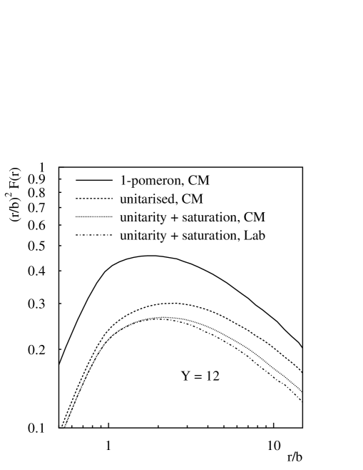
Figure 9: The onium-onium scattering amplitude, showing the frame invariance that results when both unitarity and saturation corrections are included.

and where $R_{i}$ is the normal rate of branching (i.e. without saturation). The overlap measure of saturation, $O_{i}$, is used because it is much faster to calculate, and during the Monte Carlo evolution, it will be the calculation of the saturations for each dipole which will be the limiting factor. Since the functional form of this saturation is taken from the toy model, one does not know what normalisation $\Omega$ to use for the overlaps. The procedure used for choosing $\Omega$ will be to find a value which gives a frame independent result for $F(r=0)$ ($r$ is the relative impact parameter between the colliding onia) at a single value of rapidity (which is always possible), and then to see whether this also works at other values of $r$ and rapidity. This has been done for $Y=8$, where we take $\Omega\simeq 0.33$. Reexpressing this in terms of the a more natural quantity, the probe interaction $I$, this corresponds to a modification of the branching rate by a factor $\simeq(1+I/1.3)$, which seems reasonable.

Figure 9 shows the scattering amplitudes for centre of mass and lab frames, including saturation for $Y=12$. The one-pomeron and unitarised centre of mass results are also plotted for reference. The procedure has worked insofar as the results in the two frames agree for small $r$ for the second rapidity. At larger $r$ there is still a small discrepancy between the two frames: the lab frame result is too low — there is a little bit too much saturation at large $r$ — this discrepancy is however small compared to the overall effect of saturation at those values of $r$. The same is found at all other values of rapidity (including $Y=8$). Other implementations of saturation (i.e. with different forms for eq. (33)), give very similar results, as long as the effect of saturation on branching rates is linear for small overlaps.

Figure 10: Onium-nucleus collisions (nucleus consists of two onia) in various frames: the upper set of three curves contains only unitarity corrections, while the lower set has both unitarity and saturation corrections.

As a second check on this form of saturation, one can examine onium-nucleus collisions. As well as the two lab frames discussed earlier we examine also a “centre of mass” frame (or more accurately, a frame in which the mean number of central dipoles is the same for the onium and the nucleus). Neglecting saturation one expects the $L_{O}$ frame to have the lowest unitarity corrections (since with the nucleus containing all the rapidity, it will have the largest saturation corrections), followed by the $L_{N}$ and CM frames. Figure 10 shows this ordering of the amplitudes. Once saturation is included (using exactly the same procedure as for onium-onium collisions), the three frames give very similar amplitudes, though again there is a small discrepancy at larger $r$.

It would be interesting to examine how this implementation of saturation affects the typical $S$-matrix for small impact parameters, and whether this is in accord with the arguments presented earlier. However the asymptotic $e^{-c(Y-Y_{0})^{2}/2}$ behaviour sets in only for relatively large rapidities (one needs $Y\geq 14$), and calculation of the saturation corrections at these rapidities is extremely time consuming (because the calculation time is proportional to the square of the number of dipoles) and therefore not feasible.

Considering the difference between the amplitude in the centre of mass frame with and without saturation, at small $r$, saturation seems to have a fairly small effect on the centre of mass amplitude. This is as expected from the basic argument that each onium has half the rapidity, and should be well away from saturation when unitarity corrections start to set in. At large $r$, however, the effect of saturation is bigger, and in fact of the same order as the unitarisation correction (which relates to the observation for figure 8 that at larger $r$ there is a big difference between the centre of mass and lab frame results, indicating that saturation must have a significant effect at large $r$).

Figure 11: Saturation at different stages of evolution. The maximum dipole size at a given rapidity is $c_{max}$, and $O_{max}$ is the maximum overlap of any dipole between $c_{max}$ and $c_{max}/3$ (essentially a measure of the saturation on the scale of $c_{max}$). Errors are large at large $r$ because of a lack of statistics in that region.

The dynamics involved in producing the effects saturation at large $r$ are complex: because the unitarisation corrections are small, the densities of dipoles must be small, and one might be misled into thinking that saturation corrections should unimportant. One reason why this argument fails is that there are a variety of ways in which large $r$ interaction can occur. A large dipole can be produced early in the evolution, which can then evolve to produce many other dipoles of similar size and the final density of dipoles will be indicative of the relevant saturation corrections (these evolution paths tend to also have significant unitarity corrections). Another evolution path involves only small dipoles for most of the rapidity and a branching to larger dipoles at a late stage. The evolution of the small dipoles may have been subjected to significant saturation; but once the branching occurs to large dipoles, unitarity corrections and any further saturation corrections (at the large scale) are no longer affected by what is happening on the small scale. The history of saturation can therefore have an important effect on the evolution, even though the diluteness of the final configuration might make one think one could neglect saturation. This is illustrated in the upper part of figure 11: at two values of rapidity ($y=6$ and $y=8$), the maximum dipole size, $c_{max}(y)$ is determined. The maximum overlap, $O_{max}$ is then calculated for all dipoles with size $c$, where $c_{max}>c>c_{max}/3$, in effect giving the saturation on the scale of the largest dipole. The figure shows the ratio $O_{max}(y=8)/O_{max}(y=6)$, the increase in saturation (on the largest scale), as a function of $c_{max}(y=8)/c_{max}(y=6)$, the increase in the largest dipole size. The main point is that when there is a large increase in dipole size, the ratio of the saturations drops to below one, confirming that if one looks only at the final configuration, the history of the saturation can be hidden. A similar reduction of saturation with increasing rapidity can probably also take place for the small dipoles produced from large ones (since the small ones will be more dilutely spread out).

A second effect is shown in the lower part of figure 11: the production of a large dipole tends to be a rare event. By a simple probabilistic argument, the larger the number of dipoles on a small scale, the greater the likelihood that at least one of them will branch to give a large dipole, which means that evolution paths that produce a large dipole are more likely to include an intermediate high saturation stage. The lower plot of figure 11 demonstrates this by showing the maximum saturation (again on the largest scales) at $y=4$ as a function of the ratio of the largest scales at $y=8$ and $y=4$. As the ratio of the scales increases so does the maximum intermediate saturation.

Finally in the centre of mass frame, one has the possibility of situations where one of the onia is small and moderately dense, while the other has a dilute distribution of small dipoles (the only ones which will interact with the small dense onium) at large $r$. The saturation corrections in the evolution of the small dense onium will then be of the same order as the unitarity corrections between the two at large $r$ onia, i.e. there is an asymmetry between the two onia (and arguments for neglecting saturation when unitarity corrections set in, rely on the symmetry between the two onia). This is distinct from the $r=0$ case where moderate densities of dipoles in each onium led to strongly unitarised amplitude.

The conclusions therefore, from the simple simulation of saturation effects, and from the other arguments presented above, is that at large impact parameters, it is not necessarily safe to neglect saturation corrections compared to unitarity corrections, and further that large dipoles, even when dilute, may have been produced via a high saturation stage. This might be of some concern when determining the corrections to the total cross section, which has a significant component coming from moderate to large $r$. However, to the extent that it is possible to gain any quantitative information from our simple simulation of saturation, one finds that in the total cross section, saturation corrections (up to $Y\simeq 16$) are no more than a third of the unitarity corrections.

Appendix

This section demonstrates the invariance of the one-pomeron scattering amplitude on the choice of frame. We show that it is invariant for a single dipole in each onium. Because each dipole evolves independently, and because its interaction with the other onium is independent of the other dipoles in the onium to which it belongs, this will imply that the onium-onium scattering amplitude is invariant under changes of frames at the one-pomeron level.

Let the first dipole have sources at $b_{1}$ and $b_{2}$, and the second dipole have sources at $b_{3}$ and $b_{4}$ (with the $b_{n}$ being complex variables, and $\bar{b}_{n}$ their complex conjugates). The condition for invariance of the scattering amplitude on the division of a small amount of rapidity between them is, eq. (29), which can be written as

$$\int\mathrm{d}b_{5}\mathrm{d}\bar{b}_{5}\left|\frac{b_{12}}{b_{15}b_{25}}\right|^{2}\left(\ln^{2}\left|\frac{b_{13}b_{54}}{b_{14}b_{53}}\right|^{2}+\ln^{2}\left|\frac{b_{23}b_{54}}{b_{24}b_{53}}\right|^{2}-\ln^{2}\left|\frac{b_{13}b_{24}}{b_{14}b_{23}}\right|^{2}\right)$$ (34)

$$=\int\mathrm{d}b_{5}\mathrm{d}\bar{b}_{5}\left|\frac{b_{34}}{b_{35}b_{45}}\right|^{2}\left(\ln^{2}\left|\frac{b_{13}b_{25}}{b_{15}b_{23}}\right|^{2}+\ln^{2}\left|\frac{b_{14}b_{25}}{b_{15}b_{24}}\right|^{2}-\ln^{2}\left|\frac{b_{13}b_{24}}{b_{14}b_{23}}\right|^{2}.\right)$$

To see that this holds one notes that each of the integrands (including the $\mathrm{d}b_{5}\mathrm{d}\bar{b}_{5}$ measure) is invariant under conformal transformations. The particular conformal transformation

$$b\to\frac{b+A}{Cb-1}$$ (35)

with

$$A = \frac{b_{1}-b_{2}+b_{3}-b_{4}}{b_{1}b_{3}-b_{2}b_{4}}$$ (36)

$$C = \frac{b_{1}^{-1}-b_{2}^{-1}+b_{3}^{-1}-b_{4}^{-1}}{b_{2}^{-1}b_{4}^{-1}-b_{1}^{-1}b_{3}^{-1}}$$

has the property of mapping $b_{1}\to b_{3}$, $b_{2}\to b_{4}$, $b_{3}\to b_{1}$ and $b_{4}\to b_{2}$, thus converting the lower integral in eq. (Appendix) to the upper integral (and vice-versa). Since the integrands are invariant under conformal transformations, this proves the equality, and therefore the invariance of the one-pomeron onium-onium scattering amplitude on the frame in which the calculation is performed, if the evolution is carried out using the dipole kernel and the interaction is by two gluon exchange.

References

- [1] Y. Y. Balitskiǐ and L. N. Lipatov, Sov. Phys. JETP 28 (1978) 822.
- [2] E. A. Kuraev, L. N. Lipatov, and V. S. Fadin, Sov. Phys. JETP 45 (1977) 199.
- [3] L. N. Lipatov, Sov. Phys. JETP 63 (1986) 904.
- [4] Y. L. Dokshitzer, Sov. Phys. JETP 46 (1977) 641.
- [5] V. N. Gribov and L. N. Lipatov, Sov. J. Nucl. Phys 15 (1972) 78.
- [6] G. Altarelli and G. Parisi, Nucl. Phys. B 126 (1977) 298.
- [7] A. H. Mueller and H. Navelet, Nucl. Phys. B 282 (1987) 727.
- [8] V.S.Fadin and L.N.Lipatov, DESY preprint 96-020, hep-ph/9602287 (1996).
- [9] A. H. Mueller, Nucl. Phys. B 415 (1994) 373.
- [10] A. H. Mueller and B. Patel, Nucl. Phys. B 425 (1994) 471.
- [11] A. H. Mueller, Nucl. Phys. B 437 (1995) 107.
- [12] Z. Chen and A. H. Mueller, Nucl. Phys. B 451 (1995) 579.
- [13] N. N. Nikolaev, B. G. Zakharov, and V. R. Zoller, JETP Lett. 59 (1994) 6.
- [14] G. P. Salam, Nucl. Phys. B 461 (1996) 512.
- [15] V. Abramovskii, V. Gribov, and O. Kancheli, Sov. J. Nucl. Phys 18 (1974) 308.
- [16] Z. Koba, H. B. Nielsen, and P. Olesen, Nucl. Phys. 40 (1972) 317.
- [17] G. P. Salam, Cavendish-HEP preprint 95/07, hep-ph/9601220 (1996).
- [18] L. V. Gribov, E. M. Levin, and M. G. Ryskin, Phys. Rep. 100 (1983) 1.
- [19] J. Koplik and A. H. Mueller, Phys. Rev. 12 (1975) 3638.
- [20] Y. Kovchegov, A. H. Mueller, and S. Wallon, in preparation.