DTP/96/40

May 1996

The Partonic Structure of the Proton
A. D. Martin

Department of Physics, University of Durham,

Durham, DH1 3LE, England

We review the latest information that is available about the parton distributions of the proton, paying particular attention to the determination of the gluon. We briefly describe the various processes that have been advocated to be a measure of the gluon. We discuss the importance of the gluon to the description of the structure function $F_{2}$ at small $x$, with emphasis on the $\ln 1/x$ resummations.

1. Parton distributions

Perturbative QCD is remarkably successful in describing the broad sweep of hard scattering processes involving the proton. A vital common ingredient is a universal set of parton distributions, $f_{i}(x,Q^{2})$, which allow all of these reactions to be calculated in terms of basic QCD subprocesses at the partonic level. $f_{i}(x,Q^{2})$ is the probability of finding parton $i$ (where $i$ may be a quark, antiquark or gluon) within the proton carrying a fraction $x$ of its momentum when probed by a particle with virtuality $Q^{2}$.

The classic way to probe the partonic structure of the proton is deep-inelastic lepton-nucleon scattering, where the lepton may be an electron, a muon or a neutrino. At high energy the differential cross-section for, say, deep-inelastic electron-proton scattering ($ep\rightarrow eX$) has the form

$$\frac{d^{2}\sigma}{dxdQ^{2}}=\frac{4\pi\alpha^{2}}{xQ^{4}}\left[y^{2}\;xF_{1}(x,Q^{2})+(1-y)\;F_{2}(x,Q^{2})\right]$$ (1)

with $Q^{2}\equiv-q^{2}$, the Bjorken $x$ variable $x=Q^{2}/2p.q$ and $y=Q^{2}/xs$, where $p$ and $q$ are the 4-momenta of the proton and virtual exchanged photon respectively. $\sqrt{s}$ is the centre-of-mass energy of the electron-proton collision. It is easy to see that the momentum fraction $x$ is the same as the Bjorken $x$. Since the struck quark acquires 4-momentum $xp+q$ we have $(xp+q)^{2}=m_{q}^{2}$. Thus $x=Q^{2}/2p.q$ in the infinite momentum frame where masses may be disregarded.

The relation between the observable structure function $F_{2}$ and the parton densities $f_{i}$ is, to $O(\alpha_{S})$, of the form

$$F_{2}(x,Q^{2})=x\sum_{q}e_{q}^{2}\int_{x}^{1}\frac{d\xi}{\xi}\;\left\{f_{q}(\xi,Q^{2})\;\left[\delta\left(1-\frac{x}{\xi}\right)\;+\frac{\alpha_{S}}{2\pi}\;C_{q}\left(\frac{x}{\xi}\right)\right]+f_{g}\left(\xi,Q^{2}\right)\;\frac{\alpha_{S}}{2\pi}\;C_{g}\left(\frac{x}{\xi}\right)\right\},$$ (2)

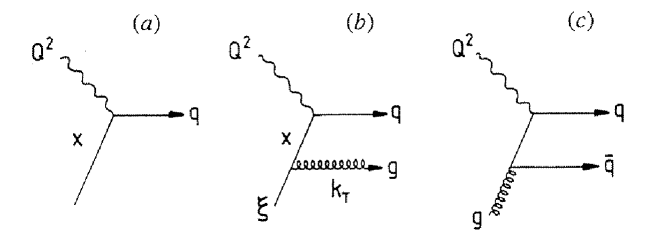
Figure 1: Partonic subprocesses which contribute to deep-inelastic scattering: (a) the lowest-order diagram, which is responsible for the quark parton model and (b), (c) QCD diagrams of first order in $\alpha_{S}$ that give contributions to $F_{2}$ which depend on the quark and gluon content respectively of the proton.

where the partonic subprocesses are shown in Fig. 1. The $O(\alpha_{S})$ QCD subprocesses shown in (b,c) have initial state collinear singularities, which are factored off into the parton densities causing them to “run” (i.e. to depend on $Q^{2}$) leaving well-behaved known coefficient functions $C_{q}$ and $C_{g}$. Due to this renormalisation, the absolute values of the parton densities are not calculable in perturbative QCD. Rather QCD determines the $Q^{2}$ dependence (or so-called scaling violations). It is given by the DGLAP evolution equations [1] which have the form

$$\frac{\partial f_{i}(x,Q^{2})}{\partial\ln Q^{2}} = \sum_{j}\int\frac{dx^{\prime}}{x^{\prime}}\;P_{ij}\left(\frac{x}{x^{\prime}}\right)\;f_{j}(x^{\prime},Q^{2})$$ (3)

$$\equiv P_{ij}\otimes f_{j},$$

where the splitting functions

$$P_{ij}=\alpha_{S}\;P_{ij}^{(1)}\;+\;\alpha_{S}^{2}\;P_{ij}^{(2)}\;+...$$ (4)

So far, the leading order (LO), $P_{ij}^{(1)}$, and next-to-leading order (NLO), $P_{ij}^{(2)}$, terms have been calculated.

Effectively, the $P_{ij}^{(1)}$ term resums the leading $\ln Q^{2}$ terms. That is the $(\alpha_{S}\ln Q^{2})^{n}$ contributions which, in an axial gauge, correspond to the sum of ladder diagrams (with $n$ rungs) in which the transverse momenta of the emitted partons (gluons) are strongly ordered along the chain (i.e. $Q^{2}\gg k_{nT}^{2}\gg...\gg k_{1T}^{2}$ in the example shown in Fig. 2). The NLO contribution corresponds to the case when a pair of momenta are comparable $k_{iT}\approx k_{i+1T}$ and we lose a power of $\ln Q^{2}$. That is $P_{ij}^{(2)}$ sums up the $\alpha_{S}^{n}\ln^{n-1}Q^{2}$ contributions. When truncating the power series at a given power of $\alpha_{S}$, say $\alpha_{S}^{m}$, the renormalisation of the $f_{i}$ introduces a scheme dependence of $O(\alpha_{S}^{m+1})$. Traditionally the $\overline{\rm MS}$ scheme is used.

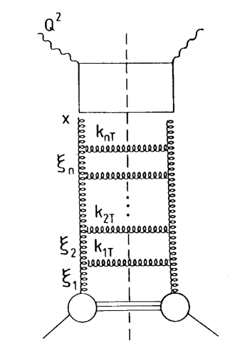
Figure 2: DGLAP evolution, which at LO sums the $(\alpha_{S}\ln Q^{2})^{n}$ contributions, corresponds for $P_{gg}$ to the sum of such ladder diagrams with the transverse momenta of the emitted gluons strongly ordered along the chain $(Q^{2}\gg k_{nT}^{2}\gg...\gg k_{1T}^{2})$. On the other hand for the BFKL $\ln 1/x$ summation (which is discussed in section 4) the ladder must be regarded as an effective ladder diagram incorporating many different contributions. In this case the $(\alpha_{S}\ln 1/x)^{n}$ contribution comes from the strongly ordered configuration $x\ll\xi_{n}\ll...\ll\xi_{1}$ but with the gluon $k_{T}$ values unordered.

2. Global analyses

The parton densities describe not only deep-inelastic scattering, but all hard scattering processes with incoming nucleons. As we have noted, the densities $f_{i}(x,Q^{2})$ have to be determined by experiment at some scale $Q^{2}=Q^{2}_{0}$. The basic procedure is to parametrize the $x$ dependence at some low $Q^{2}_{0}$, but where perturbative QCD should be applicable, and then to evolve up in $Q^{2}$ using the NLO DGLAP equations to determine $f_{i}(x,Q^{2})$ at all the values of $x,Q^{2}$ of the data. The input parameters are then determined by a global fit to the data.

To be specific the 1994/5 MRS [2, 3] and CTEQ [4] analyses took $Q^{2}_{0}$ = 4 GeV² for the input scale. We describe the MRS analyses. Similar results are obtained by CTEQ. The starting distributions are taken to be of the form

$$x\;f_{i}(x,Q^{2}_{0})=A_{i}\;x^{-\lambda_{i}}(1-x)^{\beta_{i}}\;(1+\gamma_{i}\sqrt{x}+\delta_{i}\;x)$$ (5)

for $i=g$, $u_{\rm val}$, $d_{\rm val}$ and the (total) quark sea $S$. In practice not all of the parameters $A_{i},\;\lambda_{i},\;\beta_{i},\;\gamma_{i},\;\delta_{i}$ are free. Three of the $A_{i}$ are determined by the flavour and momentum sum rules. Moreover we have some idea of the values of the $\beta_{i}$ and $\lambda_{i}$ from spectator counting rules and Regge expectations respectively. The QCD coupling is also a free parameter. It is determined primarily by the scaling violations observed in the high precision BCDMS $F_{2}^{\mu p,\mu d}$ data in the region $0.35\lower 3.01385pt\hbox{$\;\stackrel{{\scriptstyle\textstyle<}}{{\sim}}\;$}x\lower 3.01385pt\hbox{$\;\stackrel{{\scriptstyle\textstyle<}}{{\sim}}\;$}0.55$.

The flavour structure of the quark sea $S=2(\bar{u}+\bar{d}+\bar{s}+\bar{c}+...)$ is determined by data. The CCFR dimuon production data [5] imply that the strange sea is suppressed by 0.5 relative to the $u$ and the $d$ sea distributions at $Q^{2}$ = 4 GeV². The difference $\bar{d}-\bar{u}$ is arranged to be compatible with the observed NA51 [6] asymmetry in Drell-Yan production in $pp$ and $pn$ collisions. The input charm sea is determined by EMC deep-inelastic data for $F_{2}^{c}$ [7]. We assume $c=0$ for $Q^{2}<m^{2}$ and for higher $Q^{2}$ we generate $c(x,Q^{2})$ by massless evolution. The data imply $m^{2}$ = 2.7 GeV². After evolution to $Q^{2}$ = 4 GeV² we find that the charm sea, to a good approximation, satisfies $2c$ = 0.02$S$. The description of the EMC charm data by MRS(A) partons is shown in Fig. 3. Clearly this is an approximate way to treat $m_{c}\neq 0$ effects. At this meeting De Roeck [8] presented the first preliminary measurements of $F_{2}^{c}$ by the H1 collaboration. To get some idea of the future impact of these data, estimates of the preliminary measurements of $F_{2}^{c}$ at $Q^{2}$ = 13, 23 and 50 GeV² have been superimposed on the $x$ = 0.002 curve in Fig. 3. Although the present parton treatment of charm appears to be satisfactory, it is clear that future more precise data will be invaluable in the investigations of the proper treatment of $m_{c}\neq 0$ effects. In summary, the data imply that at the input scale, $Q^{2}_{0}$ = 4 GeV², the charm sea carries about 0.4% of the proton’s momentum, as compared to nearly 4% by the strange sea, 6% by the up sea and 9% by the down sea.

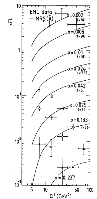
Figure 3: The description of the EMC measurements [7] of $F_{2}^{c}$ with $x\geq$ 0.024 by the MRS(A) partons [2]. The preliminary measurements of $F_{2}^{c}$ by the H1 collaboration, presented for the first time at this Conference [8], have been used to superimpose three data points to be compared with the $x$ = 0.002 curve.

Table 1: The experimental data (in the top part of table) used to determine parton distributions in the global analyses. The last column gives an indication of the main type of constraint imposed by a particular set of data. The processes in the bottom part of the table are discussed in Section 3.

	Leading-order
Process and Experiment	subprocess	Parton and $\alpha_{S}$ determination
	$\mathchar 4921\relax$
DIS $(\mu N\rightarrow\mu X)$	$\gamma^{*}q\rightarrow q$	Four structure functions $\rightarrow$
BCDMS, NMC, E665		$u+\bar{u}$, $d+\bar{d}$
$F^{\mu p}_{2},F^{\mu n}_{2}$	$\mathchar 4925\relax$	$\bar{u}+\bar{d}$, $s$ (assumed = $\bar{s}$)
DIS $(\nu N\rightarrow\mu X)$	$W^{*}q\rightarrow q^{\prime}$	but only $\int xg(x)dx\simeq 0.5$
CCFR (CDHSW)		[$\bar{u}-\bar{d}$ is not determined]
$F^{\nu N}_{2},xF^{\nu N}_{3}$	$\mathchar 4923\relax$	$\alpha_{S}$ ($x\approx$ 0.4 data)
$\mu N\rightarrow c\overline{c}X$	$\gamma^{*}c\rightarrow c$	$c\approx 0.1s$ at $Q^{2}$ = 4 GeV2
$F_{2}^{c}$, EMC
$\nu N\rightarrow\mu^{+}\mu^{-}X$	$W^{*}s\rightarrow c$	$s\approx\frac{1}{2}\bar{u}$ (or $\frac{1}{2}\bar{d}$)
CCFR	$\;\;\;\;\;\;\;\;\;\;\;\;\;\hookrightarrow\mu^{+}$
DIS (HERA)	$\gamma^{*}q\rightarrow q$	$\lambda_{g}$, $\lambda_{S}$, $\alpha_{S}$
$F^{ep}_{2}$ (H1,ZEUS)		($xg\sim x^{-\lambda_{g}},x\bar{q}\sim x^{-\lambda_{S}}$)
$pp\rightarrow\gamma X$     WA70 (UA6,	$qg\rightarrow\gamma q$	$g(x\approx 0.4)$
E706, R806, UA2, CDF)
$pN\rightarrow\mu^{+}\mu^{-}X$	$q\bar{q}\rightarrow\gamma^{*}$	$\bar{q}=...(1-x)^{\beta_{S}}$
E605
$pp,pn\rightarrow\mu^{+}\mu^{-}X$	$u\bar{u},d\bar{d}\rightarrow\gamma^{*}$	$(\bar{u}-\bar{d})$ at $x=0.18$
NA51	$u\bar{d},d\bar{u}\rightarrow\gamma^{*}$
$p\overline{p}\rightarrow W^{\pm}$ asym	$u\bar{d}\rightarrow W^{+}$	slope of $u/d$ at $x\approx 0.05$
CDF	$d\bar{u}\rightarrow W^{-}$
$p\overline{p}\rightarrow{\rm\bf jets}$	$gg$, $gq$, $q\bar{q}$	$g(0.005\lower 3.01385pt\hbox{$\;\stackrel{{\scriptstyle\textstyle<}}{{\sim}}\;$}x\lower 3.01385pt\hbox{$\;\stackrel{{\scriptstyle\textstyle<}}{{\sim}}\;$}0.1)$
CDF, D0	$\rightarrow$ 2 jets	$q(x\sim 0.2)$
		$\alpha_{S}(E_{T}\sim 100$ GeV)
$\gamma^{*}p\rightarrow{\rm\bf dijets}$	$\gamma^{*}g\rightarrow q\bar{q}$	$g(0.005\lower 3.01385pt\hbox{$\;\stackrel{{\scriptstyle\textstyle<}}{{\sim}}\;$}x\lower 3.01385pt\hbox{$\;\stackrel{{\scriptstyle\textstyle<}}{{\sim}}\;$}0.1)$, $\alpha_{S}$
H1, ZEUS	$\gamma^{*}q\rightarrow g\bar{q}$
$\gamma^{*}p\rightarrow{\rm J/}\psi X$	$\gamma^{*}g\rightarrow(c\bar{c})g$	$g$(?)
EMC, HERA
$\gamma p\rightarrow{\rm J/}\psi p$	$c\bar{c}\rightarrow c\bar{c}$	$g(x\sim 10^{-3})$
H1, ZEUS	via $gg$ exch.

The wide range of data used in the global fits is shown in the top part of Table 1, together with an indication of the most important constraints that they impose on particular partons. Fig. 4 shows the parton distributions at $Q^{2}$ = 20 GeV² corresponding to the 1994 and 1995 sets of MRS partons [2, 3], which were obtained from global fits to these data.

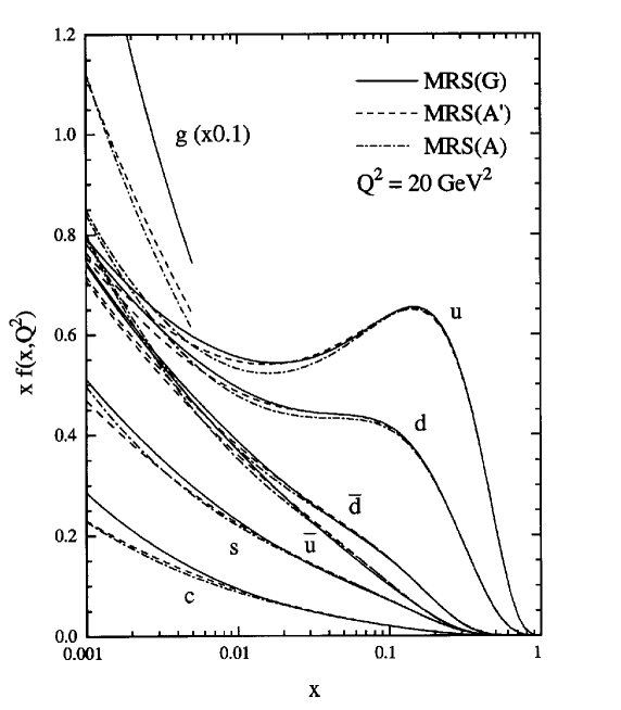
Figure 4: The 1994 [2] and 1995 [3] sets of MRS partons at $Q^{2}$ = 20 GeV². For clarity the gluon distribution (divided by a factor of 10) is only shown for $x<$ 0.005.

The differences $u-\bar{u}\equiv u_{\rm val}$ and $d-\bar{d}\equiv d_{\rm val}$ show the valence quark structures around $x\sim$ 0.1. The dominance of the gluon for $x\leq$ 0.01 is also evident. Note that the gluon is suppressed on the figure by a factor of 10. The general conclusion is that the partons are well determined for $x\lower 3.01385pt\hbox{$\;\stackrel{{\scriptstyle\textstyle>}}{{\sim}}\;$}0.02$, where data for a wide range of processes exist, except possibly the gluon which in this region is mainly constrained by prompt photon data. The gluon is clearly the crucial parton in the small $x$ domain. It is the subject of the next two sections.

3. Determination of the gluon

The gluon only contributes at leading order in prompt photon production among all the processes fitted in the global analyses, see Table 1. Its distribution is therefore not so well determined as those of the quarks. The constraints on the gluon come mainly from (i) the momentum sum rule, (ii) prompt photon production, and (iii) the scaling violations of $F_{2}$. Scaling violations impose the tightest constraint in the small $x$ region, where the gluon is the dominant parton. Then

$$\frac{\partial F_{2}}{\partial\ln Q^{2}}\approx P_{qg}\otimes g$$ (6)

where the convolution leads to the gluon being sampled at a higher value of $x$ than that at which the violation is measured. Roughly speaking an observed violation at $x$ measures $\alpha_{S}(Q^{2})$ $g(2x)$. In this way the HERA measurements of the scaling violations of $F_{2}$ at small $x$ have considerably improved our knowledge of the gluon.

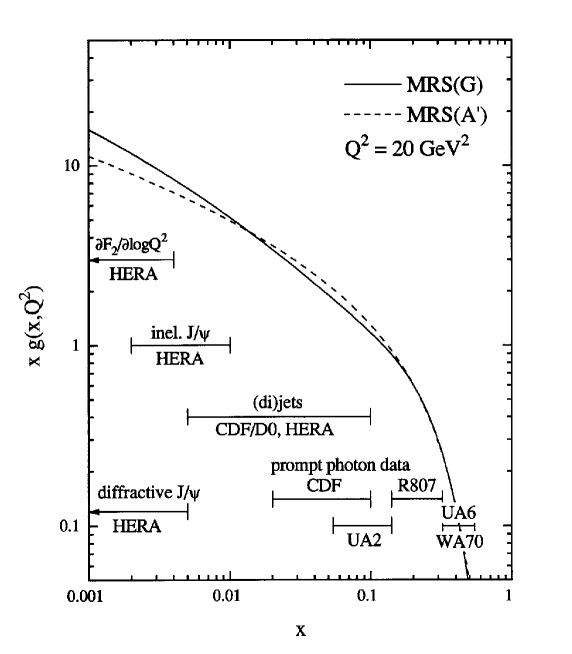
Figure 5: The $x$ intervals in which the gluon may be constrained by various sets of data. Also shown are the gluons at 20 GeV² from ref. [3].

These and other potential determinations of the gluon are summarised in Fig. 5, with an indication of the relevant $x$ ranges. We discuss the determinations in turn below.

3.1 $F_{2}$ scaling violations at HERA

In the early NLO global fits not all the parameters in

$$xg=A_{g}x^{-\lambda_{g}}\;(1-x)^{\beta g}\;(1+\gamma_{g}\sqrt{x}+\delta_{g}x)$$ (7)

were used. In particular, the data did not determine the small $x$ behaviour of the gluon. For example, $\gamma_{g}$ was set to zero, and since in the perturbative region the gluon drives the sea, via $g\rightarrow q\bar{q}$, it was assumed that $\lambda_{g}=\lambda_{S}$ at the input scale $Q^{2}_{0}$. With the advent of the HERA measurements of $F_{2}$, and their improvement year-by-year, the gluon has become better and better determined in the small $x$ region. The improvement is reflected in Table 2 in the step-by-step release of the parameters, $\lambda_{g}$ and $\gamma_{g}$, which most affect the small $x$ behaviour of the gluon. The G set of partons allowed $\lambda_{S}\neq\lambda_{g}$ for the first time, but it lead to only a marginal improvement with respect to the set A^′ in which $\lambda_{S}$ was set equal $\lambda_{g}$ [3]. The new HERA data [11, 12] exclude the G set of partons and it is interesting to note that the new parton set R1 [10] is similar to the A^′ set of partons.

Table 2: The exponents $\lambda_{i}$ of $xg\sim x^{-\lambda_{g}}$ and $xS\sim x^{-\lambda_{S}}$ at the input scale $Q^{2}_{0}$ = 4 GeV² for a sequence of MRS analyses [9, 2, 3, 10] which include more and more precise HERA data as they become available each year. The latest fit [10] has input scale $Q^{2}_{0}$ = 1 GeV² but the exponents are also given after evolution up to $Q^{2}$ = 4 GeV². The values of the parameters $\lambda_{i}$ are strongly correlated with the values of $\gamma_{i}$ (see the discussion in ref. [2]).

MRS fit		$\lambda_{g}$		$\lambda_{S}$
1993	D0	0	=	0	fixed ($\gamma_{g}=0$)
	D-	0.5	=	0.5	fixed ($\gamma_{g}=0$)
1994	A	0.3	=	0.3	free ($\gamma_{g}=0$)
1995	A′	0.17	=	0.17	free
	G	0.31		0.07	free
1996	R1	(0.17)		(0.18)	at $Q^{2}$ = 4 GeV2
		$-$0.55		0.12	at $Q^{2}_{0}$ = 1 GeV2

Traditionally the MRS and CTEQ analyses have fitted to data with $Q^{2}>5$ GeV². In the GRV approach [13, 14] valence-like forms of the parton distributions are taken at a low input scale $Q_{0}^{2}=0.34$ GeV². The original hope of this “dynamical” model was that input valence quarks would suffice and that the gluon and sea distributions would be generated radiatively. However, a sizeable valence gluon and a valence sea distribution are also required at the input scale in order to describe prompt photon and NMC deep-inelastic data respectively, which as a consequence introduces more phenomenological parameters into the GRV model. The GRV partons were found to give a good description of the HERA data down to unexpectedly low values of $Q^{2}$, namely $Q^{2}\sim 1.5$ GeV², although with the precision of the latest data there is some discrepancy at the lowest values of $x$, see Fig. 6. Motivated by the general success of the GRV (DGLAP-based) predictions, the latest MRS analysis [10] uses a lower input scale, $Q_{0}^{2}=1$ GeV², and fits to data $Q^{2}\geq 1.5$ GeV² — the resulting description of the new HERA data at the lowest values of $x$ is shown in Fig. 6. The continuous and dashed curves correspond to setting $\alpha_{S}(M_{Z}^{2})=0.113$ and 0.120 respectively. The first choice of $\alpha_{S}$ is the value determined by the scaling violations of the fixed-target deep-inelastic data, in particular the BCDMS $F_{2}^{\mu p,\mu d}$ measurements in the interval $0.35\lower 3.01385pt\hbox{$\;\stackrel{{\scriptstyle\textstyle<}}{{\sim}}\;$}x\lower 3.01385pt\hbox{$\;\stackrel{{\scriptstyle\textstyle<}}{{\sim}}\;$}0.55$ [15]. The second choice is preferred by LEP data [16], and also marginally by the HERA measurements of $F_{2}^{ep}$. The two new MRS fits have both $\lambda_{g}$ and $\lambda_{S}$ as free parameters. To see the extent to which they can be determined independently, fits are also performed with $\lambda_{g}=\lambda_{S}$. The gluon distributions of these 4 fits at $Q^{2}=5$ GeV² are shown in Fig. 7. Also shown in this plot is a representative spread of the gluons that were available in 1995. The large difference between the A^′ (with $\lambda_{S}=\lambda_{g}$) and G (with $\lambda_{S}\neq\lambda_{g}$) gluons is not present in the new fits — they all cluster about A^′. The new HERA data appear to have significantly pinned down the gluon.

Figure 6: Recent HERA measurements [11, 12] of the proton structure function $F_{2}$ versus $\ln Q^{2}$ at the lowest values of $x$. The continuous and dashed curves are the description obtained in a new preliminary MRS global analysis with the QCD coupling taken to be such that $\alpha_{S}(M_{Z}^{2})=0.113$ and 0.120 respectively [10]. The dotted curve is the prediction obtained from the GRV partons [13].

Figure 7: The gluon distribution at $Q^{2}=5$ GeV². The four continuous curves show a representative set of the gluons that were available in 1995. The four broken curves correspond to gluons obtained [10] in global analyses which include the latest HERA data — the new solutions cluster around the MRS(A^′) gluon.

3.2 Prompt photon production

The processes $pp\rightarrow\gamma X$ and $p\overline{p}\rightarrow\gamma X$ have long been regarded as a classic way to determine the gluon. The perturbative QCD formulae are now known to NLO, including the fragmentation (or Bremsstrahlung) contribution [17]. Moreover, the experiments (WA70, UA6, E706, R806, UA2, CDF) cover the entire $x$ interval from 0.6 down to 0.01. The situation therefore appears promising. However, there is a pattern of deviation in the shape of the $p_{T}$ dependence. The data are steeper in $p_{T}$ than the QCD predictions. Neither changes of scale nor the introduction of fragmentation effects can resolve the discrepancy since the various experiments probe different ranges of $x\simeq x_{T}=2p_{T}/\sqrt{s}$. On the other hand it has been shown [19] that the discrepancy can be removed by a broadening of the transverse momenta of the initial state partons (due to multigluon emission) which increases with the energy $\sqrt{s}$. A similar effect has been quantified in Drell-Yan production, but here, so far, the broadening is accounted for phenomenologically. Until the multigluon effects are calculated in QCD it is not possible to use the prompt photon data (especially those at higher energy) to pin down the gluon. The most reliable determination comes from the lower energy $pp\rightarrow\gamma X$ data of the WA70 collaboration, where the broadening is much less, but even here there is an ambiguity of some $\pm$ 25% in the value of the gluon.

3.3 Jet production at Fermilab

Dijet production in $p\overline{p}$ collisions can also, in principle, probe the small $x$ behaviour of the gluon [20, 21]. For example, if the two jets are produced with equal transverse momentum $p_{T}$ but both very forward with pseudorapidity $\eta\gg 1$ then $x_{1}\sim 1$ and $x_{2}\sim(2p_{T}/\sqrt{s})\exp(-\eta)\ll 1$. Detailed NLO calculations [21] show that at $\sqrt{s}=1.8$ TeV the gluon can be probed in this way in the range $0.005<x_{g}<0.05$. However, at present the systematic errors are too large to allow any definite conclusion to be drawn.

The single jet inclusive cross section for jet transverse energies $E_{T}\sim 100$ GeV is dependent on the gluon via the $gg,gq,g\overline{q}$ initiated subprocesses. The gluon $g(x,Q^{2})$ is sampled at $x\sim 2E_{T}/\sqrt{s}\sim 0.1$ (and $Q^{2}\sim E_{T}^{2}$) for centrally produced jets. However, the $E_{T}$ spectrum gives more information on the running of $\alpha_{S}(E_{T}^{2})$ than on the gluon. In fact if we take the information on the gluon from the scaling violations of $F_{2}$ at HERA, then the jet $E_{T}$ spectrum gives a sensitive measure of $\alpha_{S}$ [22]. The steeper the spectrum the larger the prediction for $\alpha_{S}$. There are indications from the medium $E_{T}$ CDF (and also from the preliminary D0) jet data that the observed spectra favour $\alpha_{S}(M_{Z}^{2})$ in the region 0.116 to 0.120 [22, 10]. Again the systematic error is the limiting factor.

3.4 Dijet production at HERA

The observation of dijets in deep inelastic scattering at HERA offers, in some respects, similar possibilities to jet production at Fermilab. Again within a single experiment it is possible to observe the running of $\alpha_{S}(k_{T}^{2})$. At HERA the LO subprocesses are the QCD Compton process $\gamma q\rightarrow gq$, and, relevant for the gluon, the $\gamma g\rightarrow q\overline{q}$ fusion reaction. The NLO contributions are known and the scheme dependence has just been quantified. Indeed Mirkes and Zeppenfeld [23] have presented to this Conference a detailed study of the jet algorithms and conclude that the cone or $k_{T}$ schemes are favoured and lead to less scale dependence than the other schemes. The clean identification and kinematic measurement of the jets is the experimental challenge.

3.5 Inelastic $J/\psi$ photoproduction

It has long been advocated that inelastic $J/\psi$ photoproduction at HERA may serve as a measure of the gluon — see, for example, ref. [24] which considers the colour-singlet model [25] for the process at LO accuracy. Recently the NLO contributions have been calculated [26, 27]. A detailed study of the spectra in the high energy range at HERA shows that the perturbative calculation is not well-behaved in the limit $p_{T}\rightarrow 0$, where $p_{T}$ is the transverse momentum of the $J/\psi$. No reliable prediction can be made in this singular boundary region without resummation of large logarithmic corrections caused by multigluon emission. If the small $p_{T}$ region is excluded from the analysis, the NLO result accounts for the energy dependence of the cross section and for the overall normalization, see Fig. 8 [27]. However, since the average momentum fraction of the partons is shifted to larger values when excluding the small-$p_{T}$ region, the sensitivity of the prediction to the small-$x$ behaviour of the gluon distribution is not very distinctive.

Figure 8: Total cross section for inelastic $J/\psi$ photoproduction as a function of the photon-proton energy for different parametrizations of the parton distribution in the proton. Experimental data from [28]. The figure is from [27].

3.6 Diffractive $J/\psi$ production at HERA

Diffractive $J/\psi$ photoproduction appears to offer a more promising way to distinguish between the gluon distributions. Since this is essentially an elastic process the cross section is a measure of the square of the gluon density. To leading order the cross section is given by [29, 30]

$$\left.\frac{d\sigma}{dt}\>(\gamma^{*}p\rightarrow J/\psi p)\right|_{0}\;=\;\frac{\Gamma_{ee}M_{\psi}^{3}\pi^{3}}{48\alpha}\>\frac{\alpha_{S}(\overline{Q}^{2})^{2}}{\overline{Q}^{8}}\;[xg(x,\overline{Q}^{2})]^{2}$$ (8)

with $\overline{Q}^{2}=\frac{1}{4}M_{\psi}^{2}$ and $x=M_{\psi}^{2}/W^{2}$, where $W$ is the $\gamma p$ c.m. energy. In a recent study [31], corrections to this formula have been calculated and comparisons with HERA data made, see Fig. 9. It was emphasized that the $W$ dependence, rather than the normalisation, was the more reliable discriminator between the gluons. The power of the method is evident from Fig. 9, which appears to favour the MRS(A^′) gluon. Further phenomenological studies of this process can be found in refs. [32, 33].

Figure 9: The measurements of the cross section for diffractive $J/\psi$ photoproduction compared with the full perturbative QCD prediction obtained from three 1994/5 sets of partons. The figure is taken from [31].

4. The gluon at small $x$

We have seen that the gluon is by far the dominant parton in the small $x$ regime. Indeed in the perturbative region it drives the entire partonic structure of the proton via the $g\rightarrow gg$ and $g\rightarrow q\overline{q}$ transitions.

So far our description of the data, including the small $x$ HERA data down to $Q^{2}=1.5$ GeV², has been based on the DGLAP resummation of LO and NLO $\ln Q^{2}$ terms. In fact the rise of $F_{2}$ with decreasing $x$ that is observed at HERA appears to be well described by the simplest approximation for the small $x$ behaviour of the gluon. If in the DGLAP evolution for gluon, we take the splitting function equal to its small $x$ limit, $P_{gg}\simeq(3\alpha_{S}/\pi)/x$, then it follows that

$$xg(x,Q^{2})\>\sim\>xg(x,Q_{0}^{2})\>\exp\left(2\>\left[\frac{36}{25}\>\ln\left(\frac{t}{t_{0}}\right)\>\ln\left(\frac{1}{x}\right)\right]^{\frac{1}{2}}\right)$$ (9)

where $t\equiv\ln(Q^{2}/\Lambda^{2})$, modulo slowly varying logarithms, provided the input $xg(x,Q_{0}^{2})$ is not singular. That is, in this double logarithm approximation, $xg$ increases faster than any power of $\ln(1/x)$, but slower than a power of $(1/x)$. This behaviour feeds through into $F_{2}$ and gives an excellent description of the data, as emphasized by Ball and Forte [34]; the steepness of the rise in $F_{2}$ can be tuned to the data by adjusting the evolution length $Q^{2}/Q_{0}^{2}$.

Does the success of the DGLAP description of the HERA data indicate the dominance of the $\ln Q^{2}$ resummations and the absence of higher twists? Such a conclusion would be premature. At small $x$, $x\lower 3.01385pt\hbox{$\;\stackrel{{\scriptstyle\textstyle<}}{{\sim}}\;$}10^{-3}$, we have, so far, only one type of data $(F_{2}^{ep})$ and there is freedom in the description, particularly as we have to supply the non-perturbative input at some scale $Q_{0}^{2}$. Clearly at sufficiently small $x$ the (NLO) DGLAP evolution will break down. When $\alpha_{S}\ln 1/x\sim 1$ we have to also resum $\alpha_{S}\ln 1/x$ contributions (or, to be more precise, a whole series of $\ln^{m}Q^{2}\ln^{n}1/x$ terms). At LO, the $(\alpha_{S}\ln 1/x)^{n}$ resummation is accomplished by the BFKL equation [35]. In a physical gauge, the $(\alpha_{S}\ln 1/x)^{n}$ term corresponds to an $n$-rung effective ladder diagram (Fig. 2) in which the soft gluon emissions are strongly-ordered in longitudinal momenta, but in which the transverse momenta are no longer ordered. Due to the latter fact we have to introduce the gluon distribution $f(x,k_{T}^{2})$ unintegrated over $k_{T}^{2}$, and anticipate a diffusion in $\ln k_{T}^{2}$ as we proceed along the gluon chain. The relation to the conventional gluon is given by

$$xg(x,Q^{2})\;=\;\int^{Q^{2}}\>\frac{dk_{T}^{2}}{k_{T}^{2}}\>f(x,k_{T}^{2}).$$ (10)

In principle, in the small $x$ domain the unintegrated distributions are the universal parton distributions which link process to process, via the $k_{T}$ factorization theorem [36]. An example of the theorem is given below in (13).

For fixed $\alpha_{S}$ the $x\rightarrow 0$ behaviour of the BFKL solution can be written in analytic form. Keeping only essential factors it behaves as

$$f(x,k_{T}^{2})\>\sim\>x^{-\lambda_{L}}\>\exp\left(\frac{-\ln^{2}(k_{T}^{2}/A^{2})}{B\ln(1/x)}\right)$$ (11)

where $\lambda_{L}$, the famous BFKL intercept, is given by $\lambda_{L}=(3\alpha_{S}/\pi)4\ln 2$. Thus we have a $x^{-\lambda_{L}}$ power-like growth accompanied by a diffusion in $\ln k_{T}^{2}$. If a physically reasonable prescription for the running of $\alpha_{S}$ is assumed then the BFKL equation may be solved numerically to yield [37] a form

$$f(x,k_{T}^{2})\>\sim\>C(k_{T}^{2})\>x^{-\lambda}$$ (12)

where $\lambda\approx 0.5$ is less sensitive to the phenomenological treatment of the infrared region, than the normalisation $C$. The BFKL prediction for the structure function $F_{2}$ is obtained using the $k_{T}$ factorization theorem [36]

$$F_{2}(x,Q^{2})\;=\;\int_{x}^{1}\>\frac{dx^{\prime}}{x^{\prime}}\>\int\>\frac{dk_{T}^{2}}{k_{T}^{2}}\>f(x^{\prime},k_{T}^{2})\>F_{2}^{\gamma g}\left(\frac{x}{x^{\prime}},k_{T}^{2},Q^{2}\right),$$ (13)

where the integration is over the kinematic variables $(x^{\prime},k_{T}^{2})$ of the virtual gluon coupling to the quark box in Fig. 2. $F_{2}^{\gamma g}$ is the off-shell gluon structure function which at LO is given by the quark box (and crossed-box) contributions to photon-gluon fusion. The BFKL approach is also found to give a satisfactory description of $F_{2}$ for small $x$. However, there are, at present, limitations to the “prediction”. We comment on the ambiguities in the BFKL calculation of $F_{2}$ below.

• Due to the diffusion of $f(x,k_{T}^{2})$ in $\ln k_{T}^{2}$ there is a significant contribution from the infrared $k_{T}^{2}$ region which is beyond the scope of perturbative QCD and which has to be included using physically motivated phenomenological forms. This leads to an uncertainty in the overall normalization of $F_{2}$, but much less in the $x$ dependence. A physically reasonable treatment of the infrared region is found to give the experimental normalization. In a sense this is equivalent to providing the non-perturbative input for DGLAP, but here the $x^{-\lambda}$ behaviour at small $x$ is prescribed.

• The BFKL equation only resums the LO $\ln 1/x$ terms. The NLO contributions are needed for a stable prediction. Sub-leading effects, which to a large extent embrace both energy-momentum conservation and angular ordering, have been shown [32, 38] to significantly reduce the value of the exponent $\lambda$.

• An underlying soft Pomeron contribution has to be included in the small $x$ region, determined by the extrapolation of the observed values of $F_{2}$ at large $x$. Again this has the effect of reducing the value of $\lambda$ apparent in $F_{2}\sim x^{-\lambda}$.

• Shadowing corrections to the BFKL equation will eventually, as $x$ decreases, suppress the $x^{-\lambda}$ growth. Although they have not yet been fully formulated, the evidence from the observed ratio of diffractive to non-diffractive deep-inelastic events, and from the persistent rise of $F_{2}$ at very low $Q^{2}\approx 2$ GeV², indicates that shadowing effects are at most 10% in the HERA regime.

• We need further studies of a unified approach which incorporates, on a sound theoretical footing, both the BFKL and DGLAP resummations.

From the above discussion it is clear that there are many issues to be resolved. We see that it will not be easy to quantify the importance of the $\ln 1/x$ BFKL-type contributions by using the effective $\lambda$ dependence of the measured values of $F_{2}$ at small $x$, that is $F_{2}\sim x^{-\lambda_{\rm eff}}$.

There has recently been much activity [39] based on expanding the anomalous dimensions $\gamma_{ij}(\alpha_{S},\omega)$ in terms of $\alpha_{S}$ and the moment variable $\omega$. For instance, for the gluon anomalous dimension, (LO) DGLAP resummation amounts to summing the terms

$$\gamma_{gg}\;=\;d_{1}\>\frac{\alpha_{S}}{\omega}\;+\;d_{2}\>\alpha_{S}\;+\;d_{3}\>\alpha_{S}\omega\;+\;\ldots,$$ (14)

whereas BFKL resums a different subset of terms

$$\gamma_{gg}\;=\;b_{1}\>\frac{\alpha_{S}}{\omega}\;+\;b_{4}\>\frac{\alpha_{S}^{4}}{\omega^{4}}\;+\;\ldots$$ (15)

with the $\omega^{-n}$ term corresponding to a $x^{-1}\log^{n-1}1/x$ contribution to $P_{gg}$ (except for $n=1$ where $P_{gg}\sim 1/x$, see (16)). Both the above expansions start with the same “double logarithm” term

$$\gamma_{gg}\;=\;\int_{0}^{1}\>dx\>x^{\omega}P_{gg}\;\approx\;\int_{0}^{1}\>dx\>x^{\omega}\>\left(\frac{d_{1}\alpha_{S}}{x}\right)\;=\;d_{1}\>\frac{\alpha_{S}}{\omega},$$ (16)

with $b_{1}=d_{1}$ which leads to the behaviour displayed in (9). Some of the first few coefficients of the BFKL expansion (15) vanish, namely $b_{2}=b_{3}=b_{5}=0$ [40]. For this reason much of the rise of $F_{2}$ with decreasing $x$ is attributed to the LO expansion of $\gamma_{qg}$

$$\gamma_{qg}\;=\;\alpha_{S}\>\left(c_{1}\;+\;c_{2}\>\frac{\alpha_{S}}{\omega}\;+\;c_{3}\>\frac{\alpha_{S}^{2}}{\omega^{2}}\;+\;\ldots\right),$$ (17)

which contributes to $F_{2}$ via $\partial F_{2}/\partial\ln Q^{2}=P_{qg}\otimes g$. All the coefficients $c_{i}$ are non-vanishing (unlike those for $\gamma_{gg}$), positive definite and large [41].

In principle, this approach appears to offer the attractive possibility of quantifying the importance of $\ln 1/x$ effects by studying DGLAP-type evolution with anomalous dimensions (and coefficient functions) which incorporate the $(\alpha_{S}/\omega)^{n}$ terms. However, it has been pointed out [42] that such a procedure masks the true dependence on contributions from the infrared region. Due to the diffusion in $\ln k_{T}^{2}$ at small $x$, an $(\alpha_{S}/\omega)^{n}$ contribution, which in DGLAP is assigned to the local point $Q^{2}$, actually samples the region of (the logarithm of) virtuality

$$\ln Q^{2}\;\pm\;(\Delta(x))^{n}$$ (18)

where $\Delta$ increases approximately as $(\ln 1/x)^{\frac{1}{2}}$. Due to the large numerical coefficient, $B=(3\alpha_{S}/\pi)56\zeta(3)$ (with $\zeta(3)=1.202$), in the diffusion term in (11), there is considerable implicit penetration into the infrared region. For example it is found that the $(\alpha_{S}/\omega)^{4}$ term samples virtualities down to $Q^{2}/100$ [42]. Thus it seems that there is no alternative but to work with the unintegrated gluon distribution and the $k_{T}$ factorization theorem and to study the effects of contributions from the infrared $k_{T}$ region explicitly.

The observable $F_{2}$ is too inclusive to show all the characteristics of the small $x$ properties of the unintegrated gluon $f(x,k_{T}^{2})$. In particular the $\ln k_{T}^{2}$ diffusion pattern is integrated over. For this reason other observables which measure properties of the final state in deep inelastic scattering have been advocated as better indicators of $\ln 1/x$ resummation effects (see, for example, the reviews listed in ref. [43]).

5. Conclusions

The universal parton distributions of the proton are well determined by a wide range of data in the region $x\lower 3.01385pt\hbox{$\;\stackrel{{\scriptstyle\textstyle>}}{{\sim}}\;$}0.02$. The exception is the gluon, which although constrained, still has some residual ambiguity. However, the scaling violations observed in the new, more precise HERA measurements of $F_{2}$ have pinned down the gluon in the small $x$ region ($x\sim 10^{-3}$). One consequence is that the GRV model which gave such an excellent description down to $Q^{2}\sim 1$ GeV², shows some systematic discrepancy. The prediction is above the new HERA measurements at the lower values of $x$, see Fig. 6. Indeed the previous spread of possible gluon behaviour at small $x$ (represented by the MRS (A^′, G), CTEQ3 and GRV curves in Fig. 7) has been narrowed in global analyses [10] incorporating the new data to give gluons similar to that of the MRS(A^′) set. Motivated by the success of the GRV approach, the latest global analysis [10] uses a lower input scale, $Q_{0}^{2}=1$ GeV².

The measurements of diffractive $J/\psi$ photoproduction at HERA were seen to also favour the gluon of the MRS(A^′) set of partons, see Fig. 9. We briefly reviewed other ways in which the gluon may be measured. Jet production at Fermilab and at HERA offer not only a constraint on the gluon, but also provide a sensitive measure of the running of $\alpha_{S}$.

Finally, we briefly discussed the perturbative QCD expectations for the behaviour of the gluon in the small $x$ region. We emphasized the importance of resumming the $(\alpha_{S}\ln 1/x)^{n}$ terms when $x$ is sufficiently small so that $\alpha_{S}\ln 1/x\sim 1$. We highlighted the problems of incorporating these effects in the description of $F_{2}$ and the necessity to use the unintegrated gluon distribution together with the $k_{T}$ factorization theorem. The dramatic improvement in the experimental measurements in the small $x$ domain serves as a challenge to provide a deeper theoretical understanding of this fascinating frontier of QCD.

It is a pleasure to thank Dick Roberts and James Stirling, and Jan Kwieciński and Peter Sutton for most enjoyable research collaborations on the structure of the proton and Misha Ryskin for valuable discussions. Also to thank our hosts in Kraków for arranging an excellent Workshop.

References

-
[1]
Yu. Dokshitzer, Soviet Phys. JETP 46 (1977) 641;
V.N. Gribov and L.N. Lipatov, Soviet J. Nucl. Phys. 15 (1972) 438, 675;
G. Altarelli and G. Parisi, Nucl. Phys. B126 (1977) 298. - [2] A.D. Martin, R.G. Roberts and W.J. Stirling, Phys. Rev. D50 (1994) 6734.
- [3] A.D. Martin, R.G. Roberts and W.J. Stirling, Phys. Lett. B354 (1995) 155.
- [4] H.L. Lai, J. Botts, J. Huston, J.G. Morfin, J.F. Owens, J.W. Qiu and W.-K. Tung, Phys. Rev. D51 (1995) 4763.
- [5] CCFR collaboration: A. Bazarko et al., Columbia University Report NEVIS-1492 (1993).
- [6] NA51 collaboration: A. Baldit et al., Phys. Lett. B332 (1994) 244.
- [7] EMCollaboration: J.J. Aubert et al., Nucl. Phys. B213 (1983) 31.
- [8] A. De Roeck, these proceedings.
- [9] A.D. Martin, R.G. Roberts and W.J. Stirling, Phys. Lett. B306 (1993) 145.
- [10] A.D. Martin, R.G. Roberts and W.J. Stirling, in preparation.
- [11] H1 collaboration: S. Aid et al., DESY report 96-039.
- [12] ZEUS collaboration: M. Derrick et al., DESY report 95-221; La Thuille Workshop, March 1996 (preliminary data).
- [13] M. Glück, E. Reya and A. Vogt, Z. Phys. C67 (1995) 433.
- [14] E. Reya, these proceedings.
- [15] A. Milsztajn and M. Virchaux, Phys. Lett. B274 (1992) 221.
- [16] S. Bethke, Nucl. Phys. B (Proc. Suppl.) 39C (1995) 198.
-
[17]
P. Aurenche, R. Baier, M. Fontannaz and D. Schiff,
Nucl. Phys. B297 (1988) 661;
H. Baer, J. Ohnemus and J.F. Owens, Phys. Lett. B234 (1990) 127; Phys.Rev. D42 (1990) 61;
L.E. Gordon and W. Vogelsang, Phys. Rev. D48 (1993) 3136; Phys. Rev. D50 (1994) 1901;
F. Aversa, P. Chiappetta, M. Greco and J.Ph. Guillet, Nucl. Phys. B327 (1989) 105;
P. Aurenche et al., Nucl. Phys. B399 (1993) 34;
M. Glück, E. Reya and A. Vogt, Phys. Rev. D48 (1993) 116. - [18] W. Vogelsang and A. Vogt, Nucl. Phys. B453 (1995) 334.
- [19] J. Huston, E. Kovacs, S. Kuhlmann, H.L. Lai, J.F. Owens and W.-K. Tung, Phys. Rev. D51 (1995) 6139.
- [20] A.D. Martin, R.G. Roberts and W.J. Stirling, Phys. Lett. B318 (1993) 184.
- [21] W.T. Giele, E.W.N. Glover and D.A. Kosower, Phys. Lett. B339 (1994) 181.
- [22] W.T. Giele, E.W.N. Glover and J. Yu, Phys. Rev. D53 (1996) 120.
- [23] E. Mirkes and D. Zeppenfeld, these proceedings.
-
[24]
A.D. Martin, C.-K. Ng and W.J. Stirling, Phys. Lett.
B191 (1987) 200;
H. Jung, G.A. Schuler and J. Terròn, Int. J. Mod. Phys. A7 (1992) 7955. - [25] E.L. Berger and D. Jones, Phys. Rev. D23 (1981) 1521.
- [26] M. Krämer, J. Zunft, J. Steegborn and P.M. Zerwas, Phys. Lett. B348 (1995) 657.
- [27] M. Krämer, Nucl. Phys. B459 (1996) 3.
- [28] H1 collaboration: S. Aid et al., Proc. of Int. Europhysics Conf. on HE Physics, Brussels, 1995.
- [29] M.G. Ryskin, Z. Phys. C57 (1993) 89.
- [30] S.J. Brodsky et al., Phys. Rev. D50 (1994) 3134.
- [31] M.G. Ryskin, R.G. Roberts, A.D. Martin and E.M. Levin, Durham preprint, DTP/95/96.
- [32] P.J. Sutton, these proceedings.
- [33] H1 collaboration: S. Aid et al., DESY report 96-037.
- [34] R.D. Ball and S. Forte, Phys. Lett. B335 (1994) 77.
-
[35]
E.A. Kuraev, L.N. Lipatov and V.S. Fadin,
Phys. Lett. B60 (1975) 50; Sov. Phys. JETP 44 (1976) 443;
Sov. Phys. JETP 45 (1977) 199.
Ya. Ya. Balitsky and L.N. Lipatov, Sov. J. Nucl. Phys. 28 (1978) 822. -
[36]
S. Catani, M. Ciafaloni and F. Hautmann, Phys. Lett.
B242 (1990) 97; Nucl. Phys. B366 (1991) 657;
J.C. Collins and R.K. Ellis, Phys. Lett. B360 (1991) 3;
E.M. Levin, M.G. Ryskin and A.G. Shuvaev, Sov. J. Nucl. Phys. 53 (1991) 657. - [37] A.J. Askew, J. Kwieciński, A.D. Martin and P.J. Sutton, Phys. Rev. D47 (1993) 3775; Phys. Rev. D49 (1994) 4402.
- [38] J. Kwieciński, A.D. Martin and P.J. Sutton, Z. Phys. C (in press).
-
[39]
R.K. Ellis, Z. Kunszt and E.M. Levin, Nucl. Phys. B420
(1994) 517;
R.K. Ellis, F. Hautmann and B.R. Webber, Phys. Lett. B348 (1995) 582;
R.D. Ball and S. Forte, Phys. Lett. B351 (1995) 513;
J.R. Forshaw, R.G. Roberts and R.S. Thorne, Phys. Lett. B356 (1995) 79. - [40] T. Jaroszewicz, Phys. Lett. B116 (1982) 291.
- [41] S. Catani and F. Hautmann, Phys. Lett. B315 (1993) 157.
- [42] M.G. Ryskin, Yu.M. Shabelski and A.G. Shuvaev, Z. Phys. C (in press).
-
[43]
J. Kwieciński, Nucl. Phys. B, Proc. Suppl. 39 BC (1995) 58;
M. Kuhlen, Proc. of DIS95 Workshop, Paris 1995, eds. J.F. Laporte and Y. Sirois, p.345.