CERN-TH/96-85

ETH-TH/96-09

hep-ph/9605270

Heavy-Quark Jets
in Hadronic Collisions
Stefano FRIXIONE

Theoretical Physics, ETH, Zurich, Switzerland

Michelangelo L. MANGANO

CERN, TH Division, Geneva, Switzerland

We present a next-to-leading order QCD calculation of the production rates of jets containing heavy quarks. This calculation is performed using the standard Snowmass jet algorithm; it therefore allows a comparison with similar results known at next-to-leading order for generic jets. As an application, we present results for the inclusive transverse energy of charm and bottom jets at the Tevatron collider, with a complete study of the dependence on the jet cone-size and of the theoretical uncertainties.

CERN-TH/96-85
May 1996

1. Introduction

The study of heavy quark production has provided some of the most interesting results in the physics of high energy hadronic collisions. The large available data sets of $b$-hadrons have been used for precise measurements of spectroscopy and lifetimes, as well as for measurements of the production rates. The associated production of jets including $b$-hadrons and $W$ vector bosons has been used for the detection of the $t$-quark. Several signals for new physics, such as an intermediate mass Higgs or the supersymmetric partners of the top quark, could manifest themselves via the presence in the final state, among other things, of jets containing $b$-quarks. A close study of the production properties of $b$-jets in QCD is therefore an important phenomenological input for many of these searches. Calculations have been performed in the past for the production of $b$-quarks at next-to-leading order (NLO) in QCD [1,2]. They have been used in comparisons with data measured at the $\rm Sp\bar{p}S$ [3] and Tevatron [4] colliders. In this paper we present a calculation of the production rates of jets including heavy quarks, at NLO in QCD. The main difference between the study of a heavy quark and a heavy-quark jet is that in the former case one is interested in the momentum of the quark itself, regardless of the properties of the event in which the quark in embedded, while in the latter case one is interested in the properties of a jet containing one or more heavy quarks, regardless of the momentum fraction of the jet carried by the quark. A priori it is expected that variables such as the $E_{\scriptscriptstyle T}$ distribution of a heavy-quark jet should be described by a finite-order QCD calculation more precisely than the $p_{\scriptscriptstyle T}$ distribution of open quarks. This is because at high momentum large logarithms $\log(\mbox{$p_{\scriptscriptstyle T}$}/m)$ appear at any order in the perturbative expansion of the open quark $p_{\scriptscriptstyle T}$ distribution, due to the emission of hard collinear gluons. These logarithms need to be resummed, using techniques such as fragmentation functions [5]. Collinear logarithms, on the other hand, are not present in the $E_{\scriptscriptstyle T}$ distribution of heavy-quark jets, since the jet $E_{\scriptscriptstyle T}$ does not depend on whether the energy is carried all by the quark or is shared among the quark and collinear gluons. The experimental measurement of the $E_{\scriptscriptstyle T}$ distribution of heavy-quark jets does not depend either on the knowledge of the heavy-quark fragmentation functions, contrary to the case of the $p_{\scriptscriptstyle T}$ distribution of open heavy quarks. Experimental systematics, such as the knowledge of decay branching ratios for heavy hadrons or of their decay spectra are also largely reduced.

The contents of this paper are as follows: in section 2 we introduce our notation, definitions, and summarize the technique used in the calculation. Section 3 presents our phenomenological results, with a complete discussion of the production rates and properties of charm and bottom jets at the Tevatron collider. Our conclusions can be found in section 4, while a thorough discussion of the technical details of the calculation is collected in the Appendix.

2. Cross sections

In this section, we briefly discuss the definition of the heavy-quark jet cross section in perturbative QCD. The interested reader will find a more detailed presentation in the Appendix.

Thanks to the factorization theorem [6], a cross section in hadronic collisions can be written in the following way

$$d\sigma^{(H_{1}H_{2})}(P_{1},P_{2})=\sum_{ab}\int dx_{1}dx_{2}f^{(H_{1})}_{a}(x_{1})f^{(H_{2})}_{b}(x_{2})d\hat{\sigma}_{ab}(x_{1}P_{1},x_{2}P_{2})\,,$$ (2.1)

where $H_{1}$ and $H_{2}$ are the incoming hadrons, $P_{1}$ and $P_{2}$ their momentum, and the sum runs over all the parton flavours which give a non-trivial contribution. The quantities $d\hat{\sigma}_{ab}$ are the subtracted partonic short-distance cross sections, which are calculable in perturbative QCD. Our aim is to evaluate these quantities for heavy-quark jet production. We will deal with $d\sigma_{ab}$, which are directly related to Feynman diagrams; $d\hat{\sigma}_{ab}$ are obtained from $d\sigma_{ab}$ by subtracting some suitable counterterms for the initial state collinear singularities [6].

In perturbative QCD, a jet has to be defined in terms of unobservable partons. The definition can be rather freely chosen, the only constraint being that it must guarantee the infra-red safeness of the cross section. In the present paper we adopt the Snowmass convention [7], whereby particles are clustered in cones of radius $R$ in the pseudorapidity-azimuthal angle plane.

The calculation of the heavy-quark jet cross section is very similar to the one of the generic-jet cross section, but two important differences have to be stressed. By its very definition, a heavy-quark jet is not flavour-blind; we have to look for those jets containing a heavy flavour. Furthermore, the mass of the heavy flavour is acting as a cutoff against final state collinear divergences; therefore, we will not have to deal with many singular contributions, which are present in the generic-jet partonic cross section.

At the leading order, the heavy-quark jet cross section in hadronic collisions gets contributions from the following partonic processes

$$g\,+\,g\,\,\rightarrow\,\,Q\,+\,\overline{Q},$$ (2.2)

$$q\,+\,\overline{q}\,\,\rightarrow\,\,Q\,+\,\overline{Q}.$$ (2.3)

At the next-to-leading order, the cross section gets contributions from the radiative correction to the processes (2.2) and (2.3), and from the tree amplitudes of the processes

$$g\,+\,g\,\,\rightarrow\,\,Q\,+\,\overline{Q}\,+\,g,$$ (2.4)

$$q\,+\,\overline{q}\,\,\rightarrow\,\,Q\,+\,\overline{Q}\,+\,g,$$ (2.5)

$$q\,+\,g\,\,\rightarrow\,\,Q\,+\,\overline{Q}\,+\,q.$$ (2.6)

In the following, we will consider the case in which the heavy-quark jet contains the heavy quark. This is by no means restrictive; the heavy antiquark obviously can be treated in the same way.

We write the leading-order contribution to the heavy-quark jet cross section as

$$d\sigma^{(0)}_{ab}={\cal S}_{2}\,{\cal M}_{ab}^{(0)}\,d\Phi_{2}\,d\mu_{\scriptscriptstyle J}\,,$$ (2.7)

where ${\cal M}_{ab}^{(0)}$ is the leading-order transition amplitude for the two-to-two process $a+b\;\mbox{$\rightarrow$}\;Q+\overline{Q}$, squared and summed over spin and colour degrees of freedom, and divided by the flux and average factors; $d\Phi_{2}$ is the two-body phase space for the $Q\overline{Q}$ pair,

$$d\mu_{\scriptscriptstyle J}\,=\,dE_{\scriptscriptstyle JT}d\eta_{\scriptscriptstyle J}d\Omega_{\scriptscriptstyle J}^{(2-2\epsilon)}$$ (2.8)

is the measure over jet variables in $4-2\epsilon$ dimensions, and ${\cal S}_{2}$ is the so-called measurement function, which defines the jet variables in terms of the partonic variables (although eq. (2.7) is completely general, the explicit form of the measurement function depends upon the merging algorithm adopted: for a discussion on the use of the measurement function in jet physics, see refs.[8,9]). In eq. (2.8) we indicated with $E_{\scriptscriptstyle JT}$ the transverse energy of the jet, and with $\eta_{\scriptscriptstyle J}$ its pseudorapidity; $d\Omega_{\scriptscriptstyle J}^{(2-2\epsilon)}$ is the angular measure in $2-2\epsilon$ dimensions. The measurement function is actually a distribution, since the jet variables are implicitly defined as entries of some $\delta$ distributions; this is the reason for the $d\mu_{\scriptscriptstyle J}$ on the RHS of eq. (2.7). The explicit form of ${\cal S}_{2}$ is given in the Appendix.

The next-to-leading order contribution is

$$d\sigma^{(1)}_{ab}=d\sigma^{(v)}_{ab}+d\sigma^{(r)}_{ab}\,,$$ (2.9)

where

$$d\sigma^{(v)}_{ab}={\cal S}_{2}\,{\cal M}_{ab}^{(v)}\,d\Phi_{2}\,d\mu_{\scriptscriptstyle J}$$ (2.10)

is the virtual part, due to the radiative corrections to the two-to-two processes, and

$$d\sigma^{(r)}_{ab}={\cal S}_{3}\,{\cal M}_{ab}^{(r)}\,d\Phi_{3}\,d\mu_{\scriptscriptstyle J}$$ (2.11)

is the real part, due to the two-to-three processes. Here $d\Phi_{3}$ is the three-body phase space for the $Q\overline{Q}$ pair plus a light parton, and ${\cal S}_{3}$ is analogous to ${\cal S}_{2}$, but takes into account the fact that, in the final state, one additional parton is present (and therefore the jet definition has to be suitably modified).

It is apparent that, at the leading order, the heavy-quark jet can only coincide with the heavy quark itself. Therefore, at the leading order, the heavy-quark jet cross section is identical to the open-heavy-quark cross section. At the next-to-leading order, the presence of a light parton in the final state enriches the kinematical structure. The heavy-quark jet can be the heavy quark, or it can contain the heavy quark and the light parton, or the heavy quark and the heavy antiquark. The heavy-quark jet cross section is therefore different from the open-heavy-quark one. Nevertheless, thanks to the non-zero mass of the quark, the structure of the singularities of the heavy-quark jet cross section is identical to the one of the open-heavy-quark cross section; a detailed proof of this statement is reported in the Appendix. We can then write the heavy-quark jet cross section at the next-to-leading order,

$$d\sigma_{ab}=d\sigma^{(0)}_{ab}+d\sigma^{(1)}_{ab}\;,$$ (2.12)

in the following way:

$$d\sigma_{ab}=d\sigma^{(open)}_{ab}+d\Delta_{ab}\,,$$ (2.13)

where $d\sigma^{(open)}_{ab}$ is the open-heavy-quark cross section, and $d\Delta_{ab}$ is implicitly defined in eq. (2.13). The Fortran code for $d\sigma^{(open)}_{ab}$ is available from the authors of ref. [2]. For the present paper, we wrote a Fortran code for the evaluation of $d\Delta_{ab}$.

3. The structure of heavy-quark jets at the Tevatron

As an application of the formalism developed so far, we present in this section some results of interest for measurements at the Fermilab 1.8 TeV Tevatron $p\bar{p}$ Collider [10]. We will consider jets containing either charm or bottom quarks. For these we will provide absolute predictions for the production rates as a function of the jet transverse energy and jet cone size $R$, and will explore the theoretical uncertainties associated to the choice of factorization ($\mu_{\rm\scriptscriptstyle{F}}$) and renormalization ($\mu_{\rm\scriptscriptstyle{R}}$) scales. Since we will be considering jets of energy much larger than the heavy-quark mass, the uncertainty associated to the mass values chosen for charm and bottom quarks is negligible, and will not be discussed. We will also study the fraction of heavy-quark jets relative to generic jets, and the fraction of $b$-jets relative to $c$-jets. For this particular distribution, we will show that most of the uncertainties related to the choice of scales cancel out in the ratio, leaving a rather accurate NLO theoretical prediction.

We consider jets produced within $|\eta|<1$, in order to simulate a realistic geometrical acceptance of the Tevatron detectors. We will use the parton distribution set MRSA^′ [11]. Our default values of the parameters entering the calculations are: $m_{c}$ = 1.5 GeV, $m_{b}$ = 4.75 GeV, $\mbox{$\mu_{\rm\scriptscriptstyle{R}}$}^{2}=\mbox{$\mu_{\rm\scriptscriptstyle{F}}$}^{2}=\mbox{$\mu_{0}$}^{2}\equiv m_{Q}^{2}+\mbox{$E_{\scriptscriptstyle T}^{2}$}$ and $R$ = 0.7.

Figure 1: $b$-jet inclusive $E_{\scriptscriptstyle T}$ distribution in $p\bar{p}$ collisions at 1.8 TeV, for $|\eta|<1$, $R=0.7$ and $\mbox{$\mu_{\rm\scriptscriptstyle{F}}$}=\mbox{$\mu_{\rm\scriptscriptstyle{R}}$}=\mbox{$\mu_{0}$}$ (solid line). For comparison, we also show the open-quark inclusive $E_{\scriptscriptstyle T}$ distribution (dashed line). The component of the jet-like contribution due to jets containing both $b$ and $\bar{b}$ is represented by the dotted line.

We start from the absolute production rates. Figure 1 shows the prediction for the $E_{\scriptscriptstyle T}$ distribution of $b$-jets at the Tevatron. For the purpose of illustration, and to provide a direct estimate of the effects calculated in this paper, we separate in the figure the contribution of the open-quark component. As indicated in the figure, the jet-like component, defined as the additional contribution to the open-quark one (the $\Delta$ term in eq. (2.13)), becomes dominant as soon as $E_{\scriptscriptstyle T}$ becomes larger than 50 GeV. We also show the part of the jet-like component due to jets that include the $b\bar{b}$ pair (we will call these $b\bar{b}$ jets). The figure suggests that for this $E_{\scriptscriptstyle T}$ range and with $R=0.7$ this is the dominant part of the jet-like component. This is consistent with the expectation that, for large enough $E_{\scriptscriptstyle T}$  and provided that the majority of the final-state generic jets are composed of primary gluons, heavy-quark jets are dominated by the process of gluon splitting, with the jet formed by the heavy-quark pair. As we will show later, the situation changes at higher $E_{\scriptscriptstyle T}$ values, where heavy quarks are mostly produced via the $s$-channel annihilation of light quarks.

Figure 2: $c$-jet inclusive $E_{\scriptscriptstyle T}$ distribution in $p\bar{p}$ collisions at 1.8 TeV, for $|\eta|<1$, $R=0.7$ and $\mbox{$\mu_{\rm\scriptscriptstyle{F}}$}=\mbox{$\mu_{\rm\scriptscriptstyle{R}}$}=\mbox{$\mu_{0}$}$ (solid line). For comparison, we also show the open-quark inclusive $E_{\scriptscriptstyle T}$ distribution (dashed line). The component of the jet-like contribution due to jets containing both $c$ and $\bar{c}$ is represented by the dotted line.

Figure 2 shows the same distributions for $c$-jets. Notice that the value of $E_{\scriptscriptstyle T}$ at which the jet-like component becomes dominant is smaller than in the case of $b$-jets. Again this is in agreement with naive expectations. The relative probability of finding a heavy-quark pair inside a high-$E_{\scriptscriptstyle T}$ gluon scales in fact like $\log(\mbox{$E_{\scriptscriptstyle T}$}/m_{Q})$ [12].

   

Figure 3: Left: relative contribution of the jet-like component in the $b$-jet inclusive $E_{\scriptscriptstyle T}$ distribution, for different values of the renormalization and factorization scales ($\mbox{$\mu_{\rm\scriptscriptstyle{R}}$}=\mbox{$\mu_{\rm\scriptscriptstyle{F}}$}=\mu$). Right: relative contribution of the jet-like component in the $b$-jet inclusive $E_{\scriptscriptstyle T}$ distribution, for various cone sizes $R$.

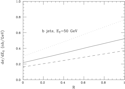
Figure 4: $b$-jet inclusive $E_{\scriptscriptstyle T}$ rate, as a function of the cone size $R$, for $E_{\scriptscriptstyle T}$ = 50 GeV (left) and $E_{\scriptscriptstyle T}$ = 100 GeV (right).

Figure 3 shows the fraction of the jet-like component of $b$-jets versus $E_{\scriptscriptstyle T}$, for various choices of factorization/renormalization scale and cone size. In the former case the dependence on scale variations is rather small, while the dependence upon the jet definition is more significant. Notice in particular that the $E_{\scriptscriptstyle T}$ value at which the jet-like component becomes dominant depends significantly on the cone size, being equal to 25, 50 and 100 GeV for $R=1$, 0.7 and 0.4 respectively.

   

Figure 5: Left: relative contribution of the jet-like component in the $c$-jet inclusive $E_{\scriptscriptstyle T}$ distribution, for different values of the renormalization and factorization scales ($\mbox{$\mu_{\rm\scriptscriptstyle{R}}$}=\mbox{$\mu_{\rm\scriptscriptstyle{F}}$}=\mu$). Right: relative contribution of the jet-like component in the $c$-jet inclusive $E_{\scriptscriptstyle T}$ distribution, for various cones sizes $R$.

Figure 6: $c$-jet inclusive $E_{\scriptscriptstyle T}$ rate, as a function of the cone size $R$, for $E_{\scriptscriptstyle T}$ = 50 GeV (left) and $E_{\scriptscriptstyle T}$ = 100 GeV (right).

The absolute rates at $E_{\scriptscriptstyle T}$ = 50 and 100 GeV as a function of the cone size are given in fig. 4. As explained in the Appendix, the cross section at $R=0$ is well defined, and it is equal to the open-quark cross section. This should be contrasted with the case of generic jets, in which the cross section at $R=0$ is not well defined, being negative at any fixed order in perturbation theory [13].

Similar results for $c$-jets are shown in figs. 5 and 6.

The strong scale dependence exhibited by the absolute rates is of the same size as the one present in the inclusive $p_{\scriptscriptstyle T}$ distribution of open heavy quarks. This scale dependence is usually attributed to the importance of the gluon splitting contribution. This process appears for the first time at ${\cal O}(\alpha_{s}^{3})$ and is therefore, strictly speaking, calculated with leading-order accuracy only. One expects therefore that in a regime in which the gluon splitting contribution is suppressed by the dynamics the scale dependence should be milder. We will show later that such a suppression takes place for high-energy heavy-quark jets. Figure 7 shows the scale dependence of the $b$-jet cross section as a function of $E_{\scriptscriptstyle T}$, for values up to 450 GeV.

Figure 7: Scale dependence of the $b$-jet $E_{\scriptscriptstyle T}$ distribution ($R=0.4$, solid lines) and of the open-quark inclusive $E_{\scriptscriptstyle T}$ distribution (dashed lines).

In the high-$E_{\scriptscriptstyle T}$ region the scale dependence is indeed reduced to the value of $20$% when the scale is varied in the range $\mbox{$\mu_{0}$}/2<\mu<2\mbox{$\mu_{0}$}$, a result consistent with the limited scale dependence of the NLO inclusive-jet cross sections [13].

In spite of the strong scale sensitivity at the smaller values of $E_{\scriptscriptstyle T}$, it is reasonable to expect that the ratio of the $b$- and $c$-jet rates be a stable quantity under scale variations. That this is indeed the case is shown in fig. 8.

Figure 8: Ratio of the $b$-jet to $c$-jet $E_{\scriptscriptstyle T}$ distributions, for different values of the renormalization and factorization scales ($\mbox{$\mu_{\rm\scriptscriptstyle{R}}$}=\mbox{$\mu_{\rm\scriptscriptstyle{F}}$}=\mu$) for $R=0.4$ (left) and $R=0.7$ (right). For comparison we also show the ratio of open quark inclusive $E_{\scriptscriptstyle T}$ distributions of $b$- and $c$-quarks.

Of direct interest for studies of heavy-flavour tagging and for searches of possible new physics is the fraction of heavy-quark jets relative to generic jets. This is also in principle the most straightforward measurement from the experimental point of view. We present in fig. 9 the ratio of the $b$-jet and inclusive-jet $E_{\scriptscriptstyle T}$ distributions [13] (a similar plot for the $c$-jet fraction is shown in fig. 10). The inclusive-jet $E_{\scriptscriptstyle T}$ cross section used here was calculated with the JETRAD program [14], using the same choices of parton densities and ($\mu_{\rm\scriptscriptstyle{R}}$,$\mu_{\rm\scriptscriptstyle{F}}$) as were adopted for the $b$-jet and $c$-jet calculations. Contrary to the figures presented so far, which showed results for the heavy quark only (i.e. no antiquark contribution), we adopt for this one the prescription used in the definition of the data presented by CDF [10]. The $b$-jets are defined there as jets containing either a $b$ or a $\bar{b}$ quark, jets containing both being counted only once. We will call these $b(\bar{b})$-jets. This distribution can be obtained by subtracting the contribution of $b\bar{b}$-jets from twice the total $b$-jet rate.

As shown in fig. 9, the normalization of the heavy-quark jet fraction depends on the choice of scale as well as on the jet definition.

Figure 9: Ratio of the $b(\bar{b})$-jet to inclusive-jet $E_{\scriptscriptstyle T}$ distributions, for different choices of renormalization and factorization scales ($\mbox{$\mu_{\rm\scriptscriptstyle{R}}$}=\mbox{$\mu_{\rm\scriptscriptstyle{F}}$}=\mu$) for $R=0.4$ (top) and $R=0.7$ (bottom). The data points for $R=0.4$ represent preliminary results from the CDF experiment [10], for which only the statistical uncertainty is shown.

In particular, the ambiguity induced by the change of scale is of ${\cal O}(2)$. While this uncertainty prevents an accurate prediction of the heavy-quark jet fractions, it is important to point out that the choice of scale for this process is not independent of the scale chosen to predict the inclusive open-quark $p_{\scriptscriptstyle T}$ distributions. Since the data on both the bottom quark [4,15] and the inclusive-jet $E_{\scriptscriptstyle T}$ spectra [16,17] strongly support the choice $\mu_{\rm\scriptscriptstyle{R}}$, $\mbox{$\mu_{\rm\scriptscriptstyle{F}}$}\sim\mbox{$\mu_{0}$}/2$, or smaller, we suggest that this is the best choice for the scales to be used in the prediction of the $b$-jet fraction.

It is interesting to notice that with this choice of scale there is good agreement between the theoretical prediction and the CDF data, at least in the case of $b$-jets. Notice also that, while the data on inclusive $b$-hadron distributions require the choice of even smaller scales (of the order of $\mbox{$\mu_{0}$}/4$ [15]), the measurement of the $b(\bar{b})$-jet rates indicates that the choice $\mu=\mbox{$\mu_{0}$}/2$ is adequate. As for the large disagreement with the charm data, we have no significant comment to make. Hopefully, additional data will soon be available, as well as estimates of the experimental systematics. Should the disagreement persist, this would indicate the presence of theoretical systematics not accounted for by the standard procedure of exploring the scale dependence of the rates. Notice that the largest contribution expected from higher-order perturbative corrections is given by the production of $c\bar{c}$ pairs from softer gluons emitted during the gluon shower evolution. However these effects have been estimated in ref. [12], and have been shown to be negligible at the energies of interest for the current measurements.

Figure 10: Ratio of the $c(\bar{c})$-jet to inclusive-jet $E_{\scriptscriptstyle T}$ distributions, for different choices of renormalization and factorization scales ($\mu_{\rm\scriptscriptstyle{R}}$=$\mu_{\rm\scriptscriptstyle{F}}$=$\mu$) for $R=0.4$ (top) and $R=0.7$ (bottom). The data points for $R=0.4$ represent preliminary results from the CDF experiment [10], for which only the statistical uncertainty is shown.

To conclude this section, we discuss the behaviour of the $b$-jet production cross section at high $E_{\scriptscriptstyle T}$. This item is interesting in view of the discrepancy reported by CDF [16] in the tail of the jet distribution. If this discrepancy could not be accommodated by new theoretical developments in QCD [18] or in the fitting of parton densities [19], a study of the flavour composition of these high-energy jets could help in understanding the nature of the phenomenon.

Figure 11: Ratio of the $b(\bar{b})$-jet to inclusive-jet $E_{\scriptscriptstyle T}$ distributions for $\mbox{$\mu_{\rm\scriptscriptstyle{R}}$}=\mbox{$\mu_{\rm\scriptscriptstyle{F}}$}=\mu/2$ and with $R=0.4$ (solid) or $R=0.7$ (dashes). The data points are preliminary CDF data [10], obtained with $R=0.4$.

Figure 11 shows the $b(\bar{b})$-jet fraction for $E_{\scriptscriptstyle T}$ values up to 450 GeV, for two different values of the cone size ($R=0.4$ and $R=0.7$) and at $\mbox{$\mu_{\rm\scriptscriptstyle{R}}$}=\mbox{$\mu_{\rm\scriptscriptstyle{F}}$}=\mbox{$\mu_{0}$}/2$. Notice that while the fraction remains constant through most of the $E_{\scriptscriptstyle T}$ range, a rise is observed above 300 GeV. To better understand the origin of this rise, we present in fig. 12a the separate contribution to the $b$-jet cross section of the three possible initial states, $gg$, $q\bar{q}$ and $qg$. Notice that the $q\bar{q}$ contribution becomes dominant for $\mbox{$E_{\scriptscriptstyle T}$}>250$ GeV. Figures 12b–d show, for each individual channel, the separate contribution of the open-quark and $b\bar{b}$-jet components. For $E_{\scriptscriptstyle T}$ large enough, the dominant component of the $gg$ and $qg$ channels is given by the $b\bar{b}$-jet contribution, because of the gluon-splitting dominance. In the case of the $q\bar{q}$ channel, on the contrary, the $b\bar{b}$-jet term is always suppressed, and most of the $b$-jets are composed of a single $b$ quark, often accompanied by a nearby gluon. We conclude that at high $E_{\scriptscriptstyle T}$ the dominant mechanism for the production of a $b$-jet is the $s$-channel annihilation of light quarks. Since at high $E_{\scriptscriptstyle T}$ mass effects are negligible, 1/5 of the jets produced in $s$-channel annihilation are $b$-jets. A simple LO calculation shows that the fraction of the two-jet rate due to $s$-channel light-quark annihilation is about 20% at $E_{\scriptscriptstyle T}$ = 450 GeV, giving an overall $b$-jet over inclusive-jet fraction of approximately 4%. This explains the rise of the $b$-fraction at high $E_{\scriptscriptstyle T}$, and provides a nice consistency check of our results. Notice also that while the probability that a gluon-jet will split into a $b\bar{b}$ pair grows at large $E_{\scriptscriptstyle T}$ faster that what predicted by the ${\cal O}(\alpha_{s}^{3})$ calculation [12], the fraction of primary gluons in the final state is so small that the overall effect on our predictions is negligible.

Figure 12: Initial state composition of the $b$-jet production processes, calculated for $\mbox{$\mu_{\rm\scriptscriptstyle{R}}$}=\mbox{$\mu_{\rm\scriptscriptstyle{F}}$}=\mu/2$ and $R=0.4$ (upper left). Different components of the production processes: $gg\;\mbox{$\rightarrow$}\;b$-jet (upper right), $q{\bar{q}}\;\mbox{$\rightarrow$}\;b$-jet (lower left) and $qg\;\mbox{$\rightarrow$}\;b$-jet (lower right).

4. Conclusions

We presented in this paper a calculation of the production of jets containing heavy quarks, at NLO in perturbative QCD. The techniques we employed represent a further elaboration of standard methods developed in recent years for the study of higher-order processes in hadronic collisions. As a phenomenological application of our results, we presented a detailed discussion of the rates and properties of charm and bottom jets produced at the Tevatron $p\bar{p}$ collider. We found that some distributions, such as the ratio of bottom to charm jets as a function of the jet transverse energy, are rather independent of the choice of renormalization and factorization scales. We presented results for the $b$- and $c$-jet fraction of inclusive jets, and discussed in detail the properties and composition of very high $E_{\scriptscriptstyle T}$ jets. We found that these vary significantly across the $E_{\scriptscriptstyle T}$ range measurable at the Tevatron. We provided predictions for the $b$-jet fractions at high $E_{\scriptscriptstyle T}$, to be compared with what could be measured by the Tevatron collider experiments.

APPENDIX A: Heavy-quark jet definition

In this appendix we report the technical details that were not explicitly given in the previous sections. In the following, we will always indicate the kinematics of a partonic process as

$$a(p_{1})+b(p_{2})\,\rightarrow\,Q(k_{1})+\overline{Q}(k_{2})+c(k),$$ (A.1)

where $c$ is the final state light parton present in the two-to-three processes.

We begin by considering the leading-order cross section, eq. (2.7). As discussed in section 2, in this case the heavy-quark jet coincides with the heavy quark. The ${\cal S}_{2}$ measurement function formally states this obvious fact

$${\cal S}_{2}=\delta(E_{\scriptscriptstyle JT}-E_{\scriptscriptstyle 1T})\delta(\eta_{\scriptscriptstyle J}-\eta_{\scriptscriptstyle 1})\delta^{1-2\epsilon}(\varphi_{\scriptscriptstyle J}-\varphi_{\scriptscriptstyle 1}).$$ (A.2)

Here we denote by $E_{\scriptscriptstyle JT}$ the transverse energy of the heavy-quark jet, and with $\eta_{\scriptscriptstyle J}$ and $\varphi_{\scriptscriptstyle J}$ its pseudorapidity and azimuthal angle respectively. $E_{\scriptscriptstyle 1T}=k_{\scriptscriptstyle 1}^{0}/\cosh(\eta_{\scriptscriptstyle 1})$ is the transverse energy of the heavy quark; notice that the transverse energy is equal to the transverse momentum only in the case of massless particles.

We then turn to the next-to-leading order contribution, eq. (2.9). Due to eq. (A.2), the heavy-quark jet cross section will be different from the open-heavy-quark one only in the real part, eq. (2.11). Using the merging algorithm of ref. [7], we have

$${\cal S}_{3} = \delta(E_{\scriptscriptstyle JT}-E_{\scriptscriptstyle 1T})\delta(\eta_{\scriptscriptstyle J}-\eta_{\scriptscriptstyle 1})\delta^{1-2\epsilon}(\varphi_{\scriptscriptstyle J}-\varphi_{\scriptscriptstyle 1})$$ (A.3)

$$\phantom{xxxx}\times\theta\Bigg{(}\left|\omega_{\scriptscriptstyle 1}-\omega\right|>g(E_{\scriptscriptstyle 1T},E_{\scriptscriptstyle T})\Bigg{)}\theta\Bigg{(}\left|\omega_{\scriptscriptstyle 1}-\omega_{\scriptscriptstyle 2}\right|>g(E_{\scriptscriptstyle 1T},E_{\scriptscriptstyle 2T})\Bigg{)}$$

$$+ \delta(E_{\scriptscriptstyle JT}-E_{\scriptscriptstyle 1T}-E_{\scriptscriptstyle T})\delta\left(\eta_{\scriptscriptstyle J}-{\eta_{\scriptscriptstyle 1}E_{\scriptscriptstyle 1T}+\eta E_{\scriptscriptstyle T}\over E_{\scriptscriptstyle JT}}\right)\delta^{1-2\epsilon}\left(\varphi_{\scriptscriptstyle J}-{\varphi_{\scriptscriptstyle 1}E_{\scriptscriptstyle 1T}+\varphi E_{\scriptscriptstyle T}\over E_{\scriptscriptstyle JT}}\right)$$

$$\phantom{xxxx}\times\theta\Bigg{(}\left|\omega_{\scriptscriptstyle 1}-\omega\right|<g(E_{\scriptscriptstyle 1T},E_{\scriptscriptstyle T})\Bigg{)}$$

$$+ \delta(E_{\scriptscriptstyle JT}-E_{\scriptscriptstyle 1T}-E_{\scriptscriptstyle 2T})\delta\left(\eta_{\scriptscriptstyle J}-{\eta_{\scriptscriptstyle 1}E_{\scriptscriptstyle 1T}+\eta_{\scriptscriptstyle 2}E_{\scriptscriptstyle 2T}\over E_{\scriptscriptstyle JT}}\right)\delta^{1-2\epsilon}\left(\varphi_{\scriptscriptstyle J}-{\varphi_{\scriptscriptstyle 1}E_{\scriptscriptstyle 1T}+\varphi_{\scriptscriptstyle 2}E_{\scriptscriptstyle 2T}\over E_{\scriptscriptstyle JT}}\right)$$

$$\phantom{xxxx}\times\theta\Bigg{(}\left|\omega_{\scriptscriptstyle 1}-\omega_{\scriptscriptstyle 2}\right|<g(E_{\scriptscriptstyle 1T},E_{\scriptscriptstyle 2T})\Bigg{)},$$

where

$$g(x,y)={x+y\over max(x,y)}R$$ (A.4)

and

$$\left|\omega_{i}-\omega_{j}\right|=\sqrt{(\eta_{i}-\eta_{j})^{2}+(\varphi_{i}-\varphi_{j})^{2}}\,.$$ (A.5)

In eq. (A.4), $R$ is the usual jet-resolution parameter, which defines the cone size in the pseudorapidity-azimuthal angle plane. The quantities appearing in previous equations are expressed in the laboratory frame.

It is well known that perturbatively calculated QCD cross sections have a divergent behaviour even after the ultraviolet renormalization, in those regions in which a massless parton is soft or collinear to another massless parton. These singularities cancel after the virtual part, the real part and the collinear counterterms are added together. To perform this cancellation analytically is therefore important, in order to disentangle the various singular contributions to the cross section. To this end, the preliminary step in our formalism is to study the behaviour of the measurements functions in the soft and collinear regions. In the case at hand, the only non-trivial case is the one of the ${\cal S}_{3}$ function, since the two-to-three processes are the only ones in which a massless parton is emitted. It is straightforward to see that the following equations hold

$$\lim_{k^{0}\mbox{$\rightarrow$}0}{\cal S}_{3} = {\cal S}_{2}\,,$$ (A.6)

$$\lim_{\vec{k}\mbox{$\rightarrow$}\vec{k}_{1}}{\cal S}_{3}=\lim_{\vec{k}\mbox{$\rightarrow$}\vec{k}_{2}}{\cal S}_{3} = {\cal S}_{2}\,.$$ (A.7)

This properties guarantee the infra-red safeness of the heavy-quark jet cross section. Notice that, due to the fact that the heavy quark is massive, we do not have to care about the final state collinear emission, which is relevant, on the other hand, for the generic-jet cross section calculations.

We now have to disentangle the singularities appearing in the heavy-quark jet cross section. For this purpose, we use the same method as was recently presented in ref. [9]. We parametrize the four-momentum of the outgoing light parton as

$$k={\sqrt{S}\over 2}\xi(1,\sqrt{1-y^{2}}\,\vec{e}_{\scriptscriptstyle T},y)\,,$$ (A.8)

where $\vec{e}_{\scriptscriptstyle T}$ is a $(2-2\epsilon)$-dimensional unitary vector in the transverse momentum space, $-1\leq y\leq 1$ and $0\leq\xi\leq\xi_{\scriptscriptstyle L}$; the collinear and soft limits are $y\mbox{$\rightarrow$}\pm 1$ and $\xi\mbox{$\rightarrow$}0$ respectively. With this parametrization, we have

$$E_{\scriptscriptstyle T}={\sqrt{S}\over 2}\xi\sqrt{1-y^{2}}\,.$$ (A.9)

Defining

$$d\Phi^{(n)}(k)={d^{n-1}k\over(2\pi)^{n-1}2k^{0}}\,,$$ (A.10)

we get

$$E_{\scriptscriptstyle T}^{-2}d\Phi^{(4-2\epsilon)}(k)={1\over 2(2\pi)^{3-2\epsilon}}\left({\sqrt{S}\over 2}\right)^{-2\epsilon}\xi^{-1-2\epsilon}\left(1-y^{2}\right)^{-1-\epsilon}d\xi dyd\Omega^{(2-2\epsilon)}\,,$$ (A.11)

where $d\Omega^{(2-2\epsilon)}$ is the angular measure in $2-2\epsilon$ dimensions. This form is suitable for disentangling the singular contributions to the real cross section. We use the identity

$$\xi^{-1-2\epsilon}\left(1-y^{2}\right)^{-1-\epsilon}={\cal D}(\xi,y)+{\cal R}(\xi,y)+{\cal O}(\epsilon),$$ (A.12)

where

$${\cal D}(\xi,y) = -{\xi_{cut}^{-2\epsilon}\over 2\epsilon}\delta(\xi)\left(1-y^{2}\right)^{-1-\epsilon}$$ (A.13)

$$- {(2y_{cut})^{-\epsilon}\over 2\epsilon}\left[\delta(1-y)+\delta(1+y)\right]\left[\left({1\over\xi}\right)_{c}-2\epsilon\left({\log\xi\over\xi}\right)_{c}\right],$$

$${\cal R}(\xi,y) = {1\over 2}\left({1\over\xi}\right)_{c}\left[\left({1\over 1-y}\right)_{c}+\left({1\over 1+y}\right)_{c}\right].$$ (A.14)

The distributions in eqs. (A.13) and (A.14) are defined as follows

$$\Bigg{\langle}\left({1\over\xi}\right)_{c},f\Bigg{\rangle} = \int_{0}^{1}d\xi\,{f(\xi)-f(0)\theta(\xi_{cut}-\xi)\over\xi}\,,$$ (A.15)

$$\Bigg{\langle}\left({1\over 1-y}\right)_{c},f\Bigg{\rangle} = \int_{-1}^{1}dy\,{f(y)-f(1)\theta(y-1+y_{cut})\over 1-y}\,,$$ (A.16)

$$\Bigg{\langle}\left({1\over 1+y}\right)_{c},f\Bigg{\rangle} = \int_{-1}^{1}dy\,{f(y)-f(-1)\theta(-y-1+y_{cut})\over 1+y}\,,$$ (A.17)

where $0<\xi_{cut}\leq 1$ and $0<y_{cut}\leq 2$ are arbitrary parameters, which can be freely chosen to improve the convergence of the results in the numerical computations. Writing the three-body phase space as

$$d\Phi_{3}=E_{\scriptscriptstyle T}^{2}\,d\tilde{\Phi}_{2}\,E_{\scriptscriptstyle T}^{-2}\,d\Phi^{(4-2\epsilon)}(k)\;,$$ (A.18)

(by construction, $d\tilde{\Phi}_{2}$ is basically identical to the two-body phase space for the $Q\bar{Q}$ pair introduced in eq. (2.7), except for the delta over the four-momentum, which in the present case reads $\delta(p_{1}+p_{2}-k_{1}-k_{2}-k)$), we can exploit eqs. (A.11) and (A.12) to write eq. (2.11) as follows (we neglect ${\cal O}(\epsilon)$ terms)

$$d\sigma^{(r)}_{ab} = {\cal S}_{3}{\cal M}_{ab}^{(r)}\,E_{\scriptscriptstyle T}^{2}\,d\tilde{\Phi}_{2}\,{1\over 2(2\pi)^{3-2\epsilon}}\left({\sqrt{S}\over 2}\right)^{-2\epsilon}{\cal D}(\xi,y)d\xi dyd\Omega^{(2-2\epsilon)}d\mu_{\scriptscriptstyle J}$$ (A.19)

$$+ {\cal S}_{3}{\cal M}_{ab}^{(r)}\,E_{\scriptscriptstyle T}^{2}\,d\tilde{\Phi}_{2}\,{1\over 2(2\pi)^{3-2\epsilon}}\left({\sqrt{S}\over 2}\right)^{-2\epsilon}{\cal R}(\xi,y)d\xi dyd\Omega^{(2-2\epsilon)}d\mu_{\scriptscriptstyle J}\,.\phantom{aaaa}$$

The measurement function ${\cal S}_{3}$ in the first term on the RHS of eq. (A.19) can be substituted with ${\cal S}_{2}$. In fact, the $\delta(\xi)$ and $\delta(1\pm y)$ contained in the factor ${\cal D}(\xi,y)$ allow us to take the soft and collinear limits of that term, that is, to exploit eqs. (A.6) and (A.7). We can also write

$${\cal S}_{3}={\cal S}_{2}+\widetilde{{\cal S}}_{3}$$ (A.20)

where

$$\widetilde{{\cal S}}_{3} = \delta(E_{\scriptscriptstyle JT}-E_{\scriptscriptstyle 1T})\delta(\eta_{\scriptscriptstyle J}-\eta_{\scriptscriptstyle 1})\delta^{1-2\epsilon}(\varphi_{\scriptscriptstyle J}-\varphi_{\scriptscriptstyle 1})$$ (A.21)

$$\phantom{xxxx}\times\Bigg{[}-\theta\Bigg{(}\left|\omega_{\scriptscriptstyle 1}-\omega\right|<g(E_{\scriptscriptstyle 1T},E_{\scriptscriptstyle T})\Bigg{)}-\theta\Bigg{(}\left|\omega_{\scriptscriptstyle 1}-\omega_{\scriptscriptstyle 2}\right|<g(E_{\scriptscriptstyle 1T},E_{\scriptscriptstyle 2T})\Bigg{)}\Bigg{]}$$

$$+ \delta(E_{\scriptscriptstyle JT}-E_{\scriptscriptstyle 1T}-E_{\scriptscriptstyle T})\delta\left(\eta_{\scriptscriptstyle J}-{\eta_{\scriptscriptstyle 1}E_{\scriptscriptstyle 1T}+\eta E_{\scriptscriptstyle T}\over E_{\scriptscriptstyle JT}}\right)\delta^{1-2\epsilon}\left(\varphi_{\scriptscriptstyle J}-{\varphi_{\scriptscriptstyle 1}E_{\scriptscriptstyle 1T}+\varphi E_{\scriptscriptstyle T}\over E_{\scriptscriptstyle JT}}\right)$$

$$\phantom{xxxx}\times\theta\Bigg{(}\left|\omega_{\scriptscriptstyle 1}-\omega\right|<g(E_{\scriptscriptstyle 1T},E_{\scriptscriptstyle T})\Bigg{)}$$

$$+ \delta(E_{\scriptscriptstyle JT}-E_{\scriptscriptstyle 1T}-E_{\scriptscriptstyle 2T})\delta\left(\eta_{\scriptscriptstyle J}-{\eta_{\scriptscriptstyle 1}E_{\scriptscriptstyle 1T}+\eta_{\scriptscriptstyle 2}E_{\scriptscriptstyle 2T}\over E_{\scriptscriptstyle JT}}\right)\delta^{1-2\epsilon}\left(\varphi_{\scriptscriptstyle J}-{\varphi_{\scriptscriptstyle 1}E_{\scriptscriptstyle 1T}+\varphi_{\scriptscriptstyle 2}E_{\scriptscriptstyle 2T}\over E_{\scriptscriptstyle JT}}\right)$$

$$\phantom{xxxx}\times\theta\Bigg{(}\left|\omega_{\scriptscriptstyle 1}-\omega_{\scriptscriptstyle 2}\right|<g(E_{\scriptscriptstyle 1T},E_{\scriptscriptstyle 2T})\Bigg{)},$$

having used the identity

$$\theta(a>b)\theta(c>d)=1-\theta(a<b)-\theta(c<d)+\theta(a<b)\theta(c<d)$$ (A.22)

in the first term on the RHS of eq. (A.3). Notice that the first term on the RHS of eq. (A.21) should also have a contribution of the kind

$$\theta\Bigg{(}\left|\omega_{\scriptscriptstyle 1}-\omega\right|<g(E_{\scriptscriptstyle 1T},E_{\scriptscriptstyle T})\Bigg{)}\theta\Bigg{(}\left|\omega_{\scriptscriptstyle 1}-\omega_{\scriptscriptstyle 2}\right|<g(E_{\scriptscriptstyle 1T},E_{\scriptscriptstyle 2T})\Bigg{)}.$$ (A.23)

Nevertheless, this quantity is always equal to zero, since otherwise it would be possible to merge in a jet all three particles in the final state. Equation (A.19) therefore becomes

$$d\sigma^{(r)}_{ab} = {\cal S}_{2}{\cal M}_{ab}^{(r)}\,E_{\scriptscriptstyle T}^{2}\,d\tilde{\Phi}_{2}\,{1\over 2(2\pi)^{3-2\epsilon}}\left({\sqrt{S}\over 2}\right)^{-2\epsilon}{\cal D}(\xi,y)d\xi dyd\Omega^{(2-2\epsilon)}d\mu_{\scriptscriptstyle J}$$ (A.24)

$$+ {\cal S}_{2}{\cal M}_{ab}^{(r)}\,E_{\scriptscriptstyle T}^{2}\,d\tilde{\Phi}_{2}\,{1\over 2(2\pi)^{3-2\epsilon}}\left({\sqrt{S}\over 2}\right)^{-2\epsilon}{\cal R}(\xi,y)d\xi dyd\Omega^{(2-2\epsilon)}d\mu_{\scriptscriptstyle J}$$

$$+ \widetilde{{\cal S}}_{3}{\cal M}_{ab}^{(r)}\,E_{\scriptscriptstyle T}^{2}\,d\tilde{\Phi}_{2}\,{1\over 2(2\pi)^{3-2\epsilon}}\left({\sqrt{S}\over 2}\right)^{-2\epsilon}{\cal R}(\xi,y)d\xi dyd\Omega^{(2-2\epsilon)}d\mu_{\scriptscriptstyle J}\,.\phantom{aaa}$$

Using again eqs. (A.12) and (A.18) we finally get

$$d\sigma^{(r)}_{ab}=d\sigma^{(r,open)}_{ab}+d\Delta_{ab}\,,$$ (A.25)

with

$$d\sigma^{(r,open)}_{ab} = {\cal S}_{2}{\cal M}_{ab}^{(r)}\,d\Phi_{3}\,d\mu_{\scriptscriptstyle J}\,,$$ (A.26)

$$d\Delta_{ab} = \widetilde{{\cal S}}_{3}{\cal M}_{ab}^{(r)}E_{\scriptscriptstyle T}^{2}\,d\tilde{\Phi}_{2}\,{1\over 2(2\pi)^{3-2\epsilon}}\left({\sqrt{S}\over 2}\right)^{-2\epsilon}{\cal R}(\xi,y)d\xi dyd\Omega^{(2-2\epsilon)}d\mu_{\scriptscriptstyle J}\,.\phantom{aaa}$$ (A.27)

Equation (A.26) is just the real contribution to open-heavy-quark production. We have therefore

$$d\sigma^{(open)}_{ab}=d\sigma^{(0)}_{ab}+d\sigma^{(v)}_{ab}+d\sigma^{(r,open)}_{ab}\,,$$ (A.28)

where the first two quantities on the RHS of this equation were given in eqs. (2.7) and (2.10), respectively.

We observe that, although eq. (A.20) has a general validity, in the case of generic-jet production it is totally useless, since eq. (A.27) would display divergences due to final state collinear emission. These divergences would be cancelled by corresponding ones in eq. (A.26). On the other hand, in the heavy-quark jet case the mass of the heavy quark is acting as a cutoff against these divergences, and eq. (A.27) is finite and can be numerically integrated. In this sense, eq. (A.27) is peculiar of the heavy-quark jet cross section. Notice finally that this term vanishes when $R\;\mbox{$\rightarrow$}\;0$, that is, when no merging is performed; this is physically sensible, since in the absence of merging we expect the heavy-quark jet cross section to coincide with the open-heavy-quark one, as is formally stated by eq. (A.25).

To integrate numerically eq. (A.27), we observe that in the collinear limits $y\;\mbox{$\rightarrow$}\;\pm 1$ and in the soft limit $\xi\mbox{$\rightarrow$}0$ the quantity $\widetilde{{\cal S}}_{3}$ vanishes. It follows that the subtractions at $y=\pm 1$ and $\xi=0$, implicitly contained in the factor ${\cal R}(\xi,y)$, eq. (A.14), are actually immaterial, and we can therefore perform in eq. (A.27) the formal substitutions

$$\left({1\over 1\pm y}\right)_{c} \rightarrow {1\over 1\pm y}\,,$$ (A.29)

$$\left({1\over\xi}\right)_{c} \rightarrow {1\over\xi}\,.$$ (A.30)

Furthermore, since all divergences have been properly regulated, we can set $\epsilon=0$ in eq. (A.27). After some algebra, we get

$$d\Delta_{ab}=\widetilde{{\cal S}}_{3}{\cal M}_{ab}^{(r)}\,d\Phi_{3}\,dE_{\scriptscriptstyle JT}d\eta_{\scriptscriptstyle J}d\varphi_{\scriptscriptstyle J}\,.$$ (A.31)

Using eqs. (A.28) and (A.31) we get eq. (2.13) and the explicit form for $d\Delta_{ab}$. We finally observe that, since eq. (A.31) is free of divergences, it is suitable for numerical integration.

References

• P. Nason, S. Dawson and R. K. Ellis, Nucl. Phys. B303(1988)607; B327(1988)49;
  W. Beenakker, H. Kuijf, W.L. van Neerven and J. Smith, Phys. Rev. D40(1989)54; W. Beenakker et al., Nucl. Phys. B351(1991)507.

• M. Mangano, P. Nason and G. Ridolfi, Nucl. Phys. B373(1992)295.

• C. Albajar et al., UA1 Collaboration, Phys. Lett. B256(1991)121.

• F. Abe et al., CDF Collaboration, Phys. Rev. Lett. 68(1992)3403; 69(1992)3704; 71(1993)500, 2396, 2537; 75(1995)1451; Phys. Rev. D53(1996)1051
  S. Abachi et al., D0 Collaboration, Phys. Rev. Lett. 74(1995)3548.

• M. Cacciari and M. Greco, Nucl. Phys. B421(1994)530.

• J. C. Collins, D. E. Soper and G. Sterman, in Perturbative Quantum Chromodynamics, 1989, ed. Mueller, World Scientific, Singapore, and references therein.

• F. Aversa et al., Proceedings of the Summer Study on High Energy Physics, Research Directions for the Decade, Snowmass, CO, 1990, edited by E. Berger (World Scientific, Singapore, 1991).

• Z. Kunszt and D. E. Soper, Phys. Rev. D46(1992)192.

• S. Frixione, Z. Kunszt and A. Signer, preprint ETH-TH/95-42,
  SLAC-PUB-95-7073, hep-ph/9512328, to appear in Nucl. Phys. B.

• P. Koehn, for the CDF Collaboration, Proceedings of the 1995 CTEQ ”Workshop on Collider Physics”, Michigan State University.

• A.D. Martin, R.G. Roberts and W.J. Stirling, Phys. Rev. D50(1994)6734.

• A.H. Mueller and P. Nason, Phys. Lett. B157(1985)226; Nucl. Phys. B266(1986)265;
  M.L. Mangano and P. Nason, Phys. Lett. B285(1992)160;
  M.H. Seymour, Nucl. Phys. B436(1995)163.

• F. Aversa, P. Chiappetta, M. Greco and J.P.Guillet, Nucl. Phys. B327(1989)105, Phys. Rev. Lett. 65(1990)401;
  S. Ellis, Z. Kunszt and D. Soper, Phys. Rev. D40(1989)2188, Phys. Rev. Lett. 64(1990)2121.

• W.T. Giele, E.W.N. Glover and D.A. Kosower, Phys. Rev. Lett. 73(1994)2019.

• S. Frixione, M. Mangano, P. Nason and G. Ridolfi, Nucl. Phys. B431(1994)453.

• F. Abe et al., CDF Collaboration, Phys. Rev. Lett. 68(1992)1104; Fermilab-Pub-96/20-E, hep-ex/9601008

• G. Blazey, for the D0 Collaboration, presented at the Rencontres de Moriond, QCD and Hadronic Interactions, 24-30 March 1996.

• S. Catani, M. Mangano, P. Nason and L. Trentadue, CERN-TH/96-86, hep-ph/9604351.

• J. Huston et al., MSU-HEP-50812, hep-ph/9511386;
  E.N. Glover, A.D. Martin, R.G. Roberts and W.J. Stirling, DTP/96/22, hep-ph/9603327.