Two-loop QCD corrections to $b\to c$ transitions at zero recoil

Abstract

Complete two-loop QCD corrections to $b\to c$ transitions are presented in the limit of zero recoil. Vector and axial-vector coefficients $\eta_{A,V}$ are calculated analytically in the limit of equal beauty and charm masses, and a series appoximation is obtained for the general mass case. $\eta_{A}$ is crucial for the determination of the absolute value of the Cabibbo-Kobayashi-Maskawa matrix element $V_{cb}$. The two-loop effects enhance the one-loop corrections by 21%, removing a major theoretical uncertainty in the value of $|V_{cb}|$. Including two-loop QCD effects and previously neglected electroweak and Coulomb corrections we find $|V_{cb}|=0.0379\pm 0.0020({\rm stat})\pm 0.0025({\rm syst})\pm 0.0011({\rm theory})$.

Elements of the Cabibbo-Kobayashi-Maskawa (CKM) matrix are fundamental input parameters of the Standard Model. Their precise measurements have been the subject of vast experimental efforts and will remain prominent issues in forthcoming projects, most notably the B-factories. The values of CKM matrix elements determine the sides of the unitarity triangle and their precise knowledge is essential for the understanding of the origin of CP violation, a major puzzle of the Standard Model.

One of the directly measurable CKM parameters is the absolute value of $V_{cb}$. The experimental value can be extracted from decays of $B$ mesons produced on the $\Upsilon(4)$ resonance (ARGUS Collab. [1], CLEO Collab. [2]) or on the $Z$ resonance (ALEPH Collab. [3], DELPHI Collab. [4]).

$|V_{cb}|$ can be obtained either from the total width of semileptonic $B$ decays or from the zero-recoil extrapolation of the exclusive decay spectrum of $B\to D^{*}l\bar{\nu}$, where $l$ is an electron or muon (see [5] for a recent review). The merits of both methods and theoretical uncertainties have been discussed in ref. [6]. The inclusive approach has the advantage of larger experimental statistics; the inherent theoretical error is mainly due to inaccurate knowledge of the quark masses which enter the decay width formula. This theoretical uncertainty already dominates the experimental error and it is not obvious that it can be significantly improved (see, however, a discussion in ref. [7] and references therein).

The exclusive method, on the other hand, benefits from recent advances [6, 8] in the heavy quark effective theory (HQET) [9, 10, 11, 12]. It has been used to obtain the latest experimental result

$$|V_{cb}|=0.0385\pm 0.0021({\rm stat})\pm 0.0025({\rm syst})\pm 0.0017({\rm theory})\quad\mbox{(ref.~{}\cite[cite]{[\@@bibref{Number}{DELPHI96}{}{}]})}.$$ (1)

The exclusive method can be summarized as follows: The recoil spectrum of the $B$ meson decay is

$${{\rm d}\Gamma(B\to D^{*}l\bar{\nu})\over{\rm d}w} = f(m_{B},m_{D^{*}})|V_{cb}|^{2}{\cal F}^{2}(w)$$ (3)

$$\qquad\times\left(1+{\alpha\over\pi}\ln{M_{Z}\over m_{B}}\right),$$

where $w$ is the product of the four-velocities of the $B$ and $D^{*}$ mesons, and $f$ is a known (see e.g. [8]) function of masses of observable particles (rather than of quark masses). HQET offers a model-independent value of the hadronic matrix element for the decay $B\to D^{*}l\bar{\nu}$ at zero recoil, ${\cal F}$(1), up to perturbative corrections, to be subsequently discussed. This point is not directly accessible in the experiment due to the vanishing phase space. Fortunately, $|V_{cb}|^{2}{\cal F}^{2}(1)$ can be deduced by extrapolating the measured values at non-zero recoil, and, given the theoretical prediction for ${\cal F}(1)$, the value of $|V_{cb}|$ can be obtained. The last factor in eq. (3) approximates the electroweak corrections [13]. In case of neutral $B$ decays an additional factor $(1+\pi\alpha)$ should be included in eq. (3) (see [14] and references therein.) It represents a 2.3% enhancement of the rate due to the final state interaction between the lepton and the charged $D^{*}$ meson.

In contrast to the decay into a pseudoscalar $D$ meson, the prediction of HQET for $B\to D^{*}$ transition is free from $1/m_{b,c}$ corrections [15] by virtue of Luke’s theorem [16]. The form factor ${\cal F}(1)$ can be written as

$${\cal F}(1)=\eta_{A}\left(1+\delta_{1/m^{2}}\right),$$ (4)

where $\eta_{A}=1+{\cal O}(\alpha_{s})$ describes the perturbative QCD corrections. The mass corrections $\delta_{1/m^{2}}$ of order $1/m_{Q}^{2}$ have been examined [6, 17]. They are estimated [17] to decrease the form factor by $(5.5\pm 2.5)\%$ and their error is responsible for approximately half of the theoretical uncertainty in the value of $|V_{cb}|$ quoted in eq. (1).

The large remaining theoretical uncertainty is due to the unknown perturbative QCD corrections. The one-loop corrections are formally identical to those calculated in the context of muon decay [18]. For the heavy quark decays they give [19, 20, 12]

$$\eta_{A} = 1-{\alpha_{s}\over\pi}C_{F}\left({3\over 4}{2-\delta\over\delta}\ln(1-\delta)+2\right)$$ (6)

$$+\left({\alpha_{s}\over\pi}\right)^{2}C_{F}\eta^{(2)}_{A}+{\cal O}(\alpha_{s}^{3}),$$

where the dimensionless variable $\delta=1-m_{c}/m_{b}$ denotes the relative difference of quark masses, and $\eta^{(2)}_{A}$ represents the two-loop QCD corrections. The latter have been subject of vigorous controversy over the last few years. In the absence of an exact calculation, a renormalization group analysis has been performed [21] but its validity has been questioned in view of the small size of the logarithm of the mass ratio $m_{b}/m_{c}$ [22, 23]. The need for a full two-loop calculation of $\eta^{(2)}_{A}$ has been emphasized by many authors [21, 22, 23, 24]. The purpose of this paper is to provide this correction.

A calculation of QCD (or even QED) two-loop corrections to a fermion decay is in general very difficult. A full calculation has never been done, neither for the muon nor for a quark. However, it is at present possible to perform such an analysis at least at the zero recoil point. The advantage of this particular kinematical point is twofold. First, because of the phase-space suppression, there is no room for real radiation. Therefore, the virtual corrections are infrared finite. Second, the four vectors of the decaying and final quarks are parallel.

These two features of the zero recoil configuration allow an exact analytic solution in the case of equal masses $m_{b}$ and $m_{c}$; in the general mass case one can construct an approximate solution in the form of a power series in the relative mass difference $\delta$. In addition, the solution has a very useful symmetry with respect to the exchange $m_{b}\leftrightarrow m_{c}$. This non-trivial symmetry, valid only at zero recoil, helps to extract maximum information from the approximating series by accelerating its convergence.

The two-loop QCD diagrams relevant to this calculation are shown in fig. 1. The Lorentz structure of the decay vertex is

$$\Gamma_{\mu}=\gamma_{\mu}(1-\gamma_{5}),$$ (7)

and the vector and axial-vector parts of this coupling are modified in different ways by the QCD corrections; at zero recoil they are parametrized by two functions, $\eta_{V,A}$

$$\gamma_{\mu}\to\eta_{V}\gamma_{\mu},\qquad\gamma_{\mu}\gamma_{5}\to\eta_{A}\gamma_{\mu}\gamma_{5}.$$ (8)

Although for the decay $B\to D^{*}l\bar{\nu}$ only the axial part is relevant, for the sake of completeness we also compute $\eta_{V}$. The one-loop result for $\eta_{V}$ is known [18, 19, 20, 12].

$$\eta_{V} = 1-{\alpha_{s}\over\pi}C_{F}\left({3\over 4}{2-\delta\over\delta}\ln(1-\delta)+{3\over 2}\right)$$ (10)

$$+\left({\alpha_{s}\over\pi}\right)^{2}C_{F}\eta^{(2)}_{V}+{\cal O}(\alpha_{s}^{3}).$$

The one-loop QCD corrections contain only one color structure, proportional to $C_{F}$. At the two-loop level it is convenient to divide up the functions $\eta_{A,V}^{(2)}$ into four parts proportional to various SU(3) factors (an overall factor $C_{F}$ has been factored out):

$$\eta_{A,V}^{(2)} = C_{F}\eta_{A,V}^{F}+(C_{A}-2C_{F})\eta_{A,V}^{AF}$$ (12)

$$+T_{R}N_{L}\eta_{A,V}^{L}+T_{R}\eta_{A,V}^{H}.$$

For a general SU(N) group $C_{A}=N$; $C_{F}=(N^{2}-1)/2N$; $T_{R}=1/2$. $N_{L}$ denotes the number of the light quark flavors whose masses can be neglected. The last term contains contributions of the massive quark loops, with $b$ and $c$ quarks. We neglect the top quark; its impact is suppressed by a factor $\sim m_{b}^{2}/m_{t}^{2}$.

Among the eight coefficient functions in eq. (12) $\eta_{A,V}^{L}$ are already known [25]. They corresponds to our diagram (f) in fig. 1 with a massless fermion in the loop. In the $\overline{\rm MS}$ scheme (with $\mu=\sqrt{m_{b}m_{c}}$), adopted also in the present work, they read

$$\eta_{A}^{L} = {5\over 24}\left[{2-\delta\over\delta}\ln(1-\delta)+{44\over 15}\right],$$ (13)

$$\eta_{V}^{L} = {1\over 24}\left[{2-\delta\over\delta}\ln(1-\delta)+2\right].$$ (14)

The remaining six functions can be calculated exactly in the case of equal masses $m_{b}$ and $m_{c}$. In this limit the momenta of the leptons in the final state vanish and the vertex function becomes a two-point function with a zero momentum insertion. Such propagator-like on-shell functions are known; a systematic method of their evaluation has been worked out in ref. [26, 27]; the underlying idea is the integration by parts method [28]. This method has greatly simplified the two-loop QED calculation of $g-2$ [29, 30]. In ref. [29] the computation of two-loop functions with a low number of zero momentum insertions has been automated. For the purpose of the present calculation a new implementation of the recurrence algorithm [31] was necessary; this is because of the necessity of computing two-loop functions with large number of zero momentum insertions.

In order to go beyond the $m_{b}=m_{c}$ limit we use the variable $\delta$ as an expansion parameter. In the real world $m_{b}$ and $m_{c}$ are far from being equal; for the purpose of this work we take $m_{b}=4.8$ GeV and $m_{c}=1.44$ GeV which yields $\delta=0.7$. Coefficients of the expansion of $\eta_{A,V}$ in $\delta$ are two-point on-shell functions which can be computed using recurrence relations. In order to ensure good numerical accuracy we have computed ten terms in the $\delta$ expansion for all diagrams in fig. 1. The analytic computation of the resulting integrals was feasible only thanks to the latest achievements in symbolic manipulation programs [32].

The results we obtained are symmetric with respect to the exchange $m_{b}\leftrightarrow m_{c}$, or $\delta\to-\delta/(1-\delta)$. The resulting fact that every other term in the $\delta$ expansion can be obtained from the earlier terms provides a strong consistency check of our procedures. On the other hand, it is possible to rewrite the series expansion in a manifestly symmetric form. For this purpose we introduce a variable invariant with respect to $m_{b}\leftrightarrow m_{c}$, $\rho\equiv{\delta^{2}/(1-\delta)}$. In terms of this variable our results can be written as a rapidly convergent series and we can safely neglect terms ${\cal O}(\rho^{5})$. Quadratic and linear logarithmic terms, implicitly present in this expansion [33, 34, 35, 21], do not spoil the convergence because $\ln(m_{b}/m_{c})$ is of order unity.

For the axial-vector function $\eta_{A}^{(2)}$ we find:

$$\eta^{AF}_{A}=-{143\over 144}-{1\over 12}\pi^{2}+{1\over 6}\pi^{2}\ln 2-{1\over 4}\zeta(3)$$ (18)

$$\;\;\;+\rho\left({29\over 576}+{55\over 1728}\pi^{2}-{1\over 16}\pi^{2}\ln 2+{3\over 32}\zeta(3)\right)$$

$$\;\;\;+\rho^{2}\left(-{2509\over 17280}+{121\over 8640}\pi^{2}\right)+\rho^{3}\left({43\over 22680}-{67\over 967680}\pi^{2}\right)$$

$$\;\;\;+\rho^{4}\left(-{17933\over 50803200}+{143\over 11612160}\pi^{2}\right)$$

$$\eta^{F}_{A}=-{373\over 144}+{1\over 6}\pi^{2}$$ (21)

$$\;\;\;+\rho\left({377\over 576}-{1\over 24}\pi^{2}\right)+\rho^{2}\left(-{29\over 648}+{1\over 360}\pi^{2}\right)$$

$$\;\;\;+\rho^{3}\left({227\over 37800}-{1\over 2520}\pi^{2}\right)+\rho^{4}\left(-{649\over 672000}+{1\over 15120}\pi^{2}\right)$$

$$\eta^{H}_{A}={115\over 18}-{2\over 3}\pi^{2}$$ (24)

$$\;\;\;+\rho\left({529\over 72}-{107\over 144}\pi^{2}\right)+\rho^{2}\left(-{337\over 144}+{137\over 576}\pi^{2}\right)$$

$$\;\;\;+\rho^{3}\left(-{255313\over 75600}+{197\over 576}\pi^{2}\right)+\rho^{4}\left(-{1957573\over 3175200}+{1\over 16}\pi^{2}\right)$$

For the corrections to the vector current we find:

$$\eta^{AF}_{V}=\rho\left({377\over 576}-{3\over 64}\pi^{2}-{1\over 16}\pi^{2}\ln 2+{3\over 32}\zeta(3)\right)$$ (28)

$$\;\;\;+\rho^{2}\left(-{107\over 5760}+{1\over 288}\pi^{2}\right)+\rho^{3}\left({41\over 10080}-{31\over 46080}\pi^{2}\right)$$

$$\;\;\;+\rho^{4}\left(-{13927\over 16934400}+{169\over 1290240}\pi^{2}\right)$$

$$\eta^{F}_{V}=\rho\left({553\over 576}-{5\over 72}\pi^{2}\right)+\rho^{2}\left(-{227\over 4320}+{1\over 360}\pi^{2}\right)$$ (30)

$$\;\,+\rho^{3}\left({251\over 33600}-{1\over 2520}\pi^{2}\right)+\rho^{4}\left(-{7537\over 6048000}+{1\over 15120}\pi^{2}\right)$$

$$\eta^{H}_{V}=\rho\left({197\over 72}-{13\over 48}\pi^{2}\right)+\rho^{2}\left(-{701\over 720}+{19\over 192}\pi^{2}\right)$$ (32)

$$\;\;\;+\rho^{3}\left(-{2851\over 1008}+{55\over 192}\pi^{2}\right)+\rho^{4}\left(-{93227\over 151200}+{1\over 16}\pi^{2}\right)$$

We note that all QCD contributions to $\eta_{V}$ vanish at $m_{b}=m_{c}$ ($\rho=0$), in consequence of vector current conservation.

So far we have not discussed the renormalization procedure which led to the results in eq. (LABEL:eq:mainA,LABEL:eq:mainV). For the external quark legs we used the two-loop quark wave function renormalization constant computed in [36]. Vanishing of the terms independent of $\rho$ in eq. (LABEL:eq:mainV) serves as an independent check of the complicated expressions given in [36]. The diagrams (b1) and (b3) require mass counterterms. For these we adopted the on-shell condition. Our results are therefore in terms of the pole masses $m_{b}$ and $m_{c}$. For the coupling constant renormalization we used the $\overline{\rm MS}$ condition with the renormalization scale at the geometric mean mass $\mu=\sqrt{m_{b}m_{c}}$. It must be noted that the symmetry $m_{b}\leftrightarrow m_{c}$ is in general valid only for the unrenormalized diagrams. If the coupling constant were normalized at a different $\mu$ the final result (LABEL:eq:mainA,LABEL:eq:mainV) would not be symmetric. The geometric mean point is the only one preserving that symmetry.

Numerically, the two-loop corrections evaluate to

$$\eta_{A}^{(2)}=-0.586(2)\times C_{F}-0.909(2)\times(C_{A}-2C_{F})$$ (35)

$$\qquad+0.145\times T_{R}N_{L}-0.155(4)\times T_{R}=-0.944(5),$$

$$\eta_{V}^{(2)}=0.395(2)\times C_{F}-0.168(2)\times(C_{A}-2C_{F})$$ (37)

$$\qquad-0.010\times T_{R}N_{L}+0.107(2)\times T_{R}=0.509(5).$$

It is interesting to compare these results with an estimate based on the subset of corrections of order $\alpha_{s}^{2}\beta_{0}$ with $\beta_{0}=11-{2\over 3}n_{f}$. With $n_{f}=4$ one gets [25]

$$\eta_{A}^{(2)}=-0.908,\quad\eta_{V}^{(2)}=0.061.$$ (38)

In the axial-vector case the agreement with the full two-loop calculation is quite good. The estimate fails badly in the vector case; this is probably because of an accidental numerical cancellation in (38) which makes the estimate of $\eta_{V}^{(2)}$ very small. The full one and two-loop corrections tend to give corrections to $\eta_{V}$ with approximately half the magnitude of those to $\eta_{A}$.

Adopting $\alpha_{s}(\sqrt{m_{b}m_{c}})=0.24$, our full two loop calculation leads to the total values of $\eta_{A,V}$

$$\eta_{A} = 1-0.033-0.007=0.960\pm 0.007,$$ (39)

$$\eta_{V} = 1+0.018+0.004=1.022\pm 0.004.$$ (40)

Since the perturbative series in QCD is asymptotic, the uncertainty in the values of $\eta_{A,V}$ has been estimated by the size of the last computed terms. The central value we obtain for $\eta_{A}$ is consistent with the value given by Neubert, $\eta_{A}({\mbox{ref.~{}\cite[cite]{[\@@bibref{Number}{Neubert95}{}{}]}}})=0.965\pm 0.020$, which was adopted in the recent experimental studies. Our result reduces the error bar by a factor 3 and removes a major source of the theoretical uncertainty in $|V_{cb}|$. This error can perhaps be further decreased by choosing a different renormalization scheme, e.g. the $V$-scheme. This possibility will be examined in a future work. However, with our estimate of the perturbative two-loop corrections to $\eta_{A}$, the uncertainty in the zero recoil form factor is dominated by the error in the $1/m_{Q}^{2}$ corrections; we adopt here the value $\delta_{1/m^{2}}=-(5.5\pm 2.5)\%$ [17, 8] (for a recent discussion of these corrections see [37].) Putting this result together with our $\eta_{A}=0.960\pm 0.007$ we find for the zero recoil form factor

$${\cal F}(1)=\eta_{A}\left(1+\delta_{1/m^{2}}\right)=0.907\pm 0.026$$ (41)

We use the latest experimental data from the recent DELPHI analysis for the $B^{0}\to D^{*-}l^{+}\nu$ decay rate. We include the electroweak correction and the Coulomb enhancement, as discussed after eq. 3. They enhance the rate by $1.3\%$ and $2.3\%$, respectively. Altogether, we find

$$|V_{cb}| = 0.0379\pm 0.0020({\rm stat})$$ (43)

$$\pm 0.0025({\rm syst})\pm 0.0011({\rm theory}).$$

We see that with the decreased theoretical uncertainty further improvement in statistical and systematic accuracy can significantly increase the precision of $|V_{cb}|$ and bring us closer to overconstraining the unitarity triangle.

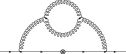
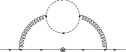
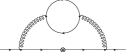
                  (a)       (b)                   (c)       (d)                   (e)       (f)

FIG. 1.: Two-loop QCD corrections to the $b\to c$ transitions at zero recoil. Symbols $\otimes$ mark the coupling of the virtual $W$ boson to the quark line.