1 Introduction

In recent years many attempts have been made to understand nucleon structure functions as measured in lepton deep-inelastic scattering (DIS). Although perturbative QCD is successful in describing the dependence of structure functions on the squared momentum transfer, their magnitude is governed by the non-perturbative physics of composite particles, and is up to now not calculable directly from QCD.

A variety of models have been invoked to describe nucleon structure functions. The so called “spectator model” is a typical covariant approach amongst them[1]. In this approach the leading twist, non-singlet quark distributions are calculated from the process in which the target nucleon splits into a valence quark, which is scattered by the virtual photon, and a spectator system carrying baryon number $2/3$. Furthermore the spectrum of spectator states is assumed to be saturated through single scalar and vector diquarks. Thus, the main ingredient of these models are covariant quark-diquark vertex functions.

Until now vertex functions have been merely parameterized such that the measured quark distributions are reproduced, and no attempts have been made to connect them to some dynamical models of the nucleon. In this work we construct the vertex functions from a model Lagrangian by solving the Bethe–Salpeter equation (BSE). However, we do not aim at a detailed, quantitative description of nucleon structure functions in the present work. Rather we outline how to extract quark-diquark vertex functions from Euclidean solutions of the BSE. In this context several simplifications are made. We consider only scalar diquarks as spectators and restrict ourselves to the $SU(2)$ flavor group. The inclusion of vector diquarks and the generalization to $SU(3)$ flavor are relatively straightforward extensions and will be left for future work.

The cross section for DIS of leptons from a nucleon is characterized by the hadronic tensor $W^{\mu\nu}(P,q)$ where $P$ and $q$ are the four-momenta of the target and exchanged virtual photon respectively. For unpolarized DIS, the hadronic tensor $W^{\mu\nu}$ is conventionally parameterized by two scalar functions $F_{1}$ and $F_{2}$. In the Bjorken limit ($-q^{2},P\cdot q\rightarrow\infty$; but finite $x\equiv-q^{2}/(2\,P\cdot q)$) in which we work throughout, both structure functions depend (up to logarithmic corrections) on $x$ only, and are related via the Callan-Gross relation: $F_{2}=2xF_{1}$.

In the scalar diquark spectator model within $SU(2)$ flavor, the valence quark distributions are extracted from the hadronic tensor (Fig. 1):

$$W^{\mu\nu}(q,P) = \left(\frac{5}{3}+\left\langle\frac{\tau_{3}}{2}\right\rangle_{N}\right)\,\frac{1}{\pi}\,\int\frac{d^{4}k}{(2\pi)^{4}i}\bar{u}(P,s)\bar{\Gamma}S(k)\gamma^{\mu}\hbox{Im}\left(S(k+q)\right)\gamma^{\nu}S(k)$$

$$\qquad\qquad\qquad\qquad\qquad\qquad\times\hbox{Im}\left(D(P-k)\right)\Gamma u(P,s),$$

where the isospin matrix element $\tau_{3}$ has to be evaluated in the nucleon isospin space. We define $u(P,s)$ as the target nucleon spinor and we use $S(k)=1/(m_{q}-k\hbox to0.0pt{\hss/})$ and $D(k)=1/(m_{D}^{2}-k^{2})$ to denote the propagators of the quark and scalar diquark, respectively. The integration runs over the quark momentum $k$, subject to on–mass–shell conditions for the diquark and the struck quark. Note that the vertex function $\Gamma$ and its PT conjugate $\bar{\Gamma}$ consist of two Lorentz scalar functions which depend on $k^{2}$ only because the diquark is on shell. In the next section we shall determine the vertex functions using a ladder Bethe-Salpeter equation.

2 Scalar–Diquark Model for Nucleon

We consider the following model lagrangian:

$${\cal L}= \bar{\psi}_{a}\left(i\partial\hbox to0.0pt{\hss/}-m_{q}\right)\psi_{a}+\partial_{\mu}\phi_{a}^{*}\partial^{\mu}\phi_{a}-m_{D}^{2}\phi_{a}^{*}\phi_{a}$$

$$+i\frac{g}{2\sqrt{2}}\epsilon^{a}_{bc}\psi^{T}_{b}C^{-1}\gamma_{5}\tau_{2}\psi_{c}\,\phi^{*}_{a}-i\frac{g}{2\sqrt{2}}\epsilon^{a}_{bc}\bar{\psi}_{b}\gamma_{5}C\tau_{2}\bar{\psi}^{T}_{c}\,\phi_{a},$$

where we have explicitly indicated color $SU(3)$ indices only. The symmetric generator $\tau_{2}$ of the flavor $SU(2)$ group acts on the iso–doublet field $\psi$ for the constituent quark carrying an invariant mass $m_{q}$. The charged scalar field $\phi$ denotes the flavor–singlet scalar diquark with invariant mass $m_{D}$.

In this model the nucleon with the momentum $P$ and spin $s/2=\pm 1/2$ is described by the BS vertex function $\Gamma$ (Fig. 2):

$$\delta_{ab}S(\eta_{q}P+q)D(\eta_{D}P-q)i\Gamma(q,P)u(P,s)=\int\frac{{\rm d}^{4}x}{(2\pi)^{3/2}}e^{ik\cdot x}\left\langle 0\left|T\psi_{a}(\eta_{q}x)\phi_{b}(-\eta_{D}x)\right|P,s\right\rangle,$$ (3)

where we set the weight factors to the classical values: $\eta_{q}=m_{q}/(m_{q}+m_{D})$ and $\eta_{D}=m_{D}/(m_{q}+m_{D})$. Then the vertex function $\Gamma$ obeys in the ladder approximation the following BSE (Fig.3):

$$\Gamma(q,P)=g^{2}\int\frac{{\rm d}^{4}k}{(2\pi)^{4}i}S(-k-q-(\eta_{q}-\eta_{D})P)S(\eta_{q}P+k)D(\eta_{D}P-k)\Gamma(k,P).$$ (4)

To solve the BSE for positive energy nucleon states we are free to choose the following Dirac matrix structure:

$$\Gamma(q,P)=\left[f_{1}(q,P)+\left(-\frac{P\cdot q}{P^{2}}+\frac{q\hbox to0.0pt{\hss/}}{\sqrt{P^{2}}}\right)f_{2}(q,P)\right]\Lambda^{(+)}(P),$$ (5)

with $\Lambda^{+}(P)=1/2(1+P\hbox to0.0pt{\hss/}/\sqrt{P^{2}})$, the projector onto positive energy nucleon states.

We assume that the diquark and the nucleon are stable, namely $m_{D}<2m_{q}$ and $\sqrt{P^{2}}<m_{q}+m_{D}$. We then perform the Wick rotation of the relative energy variable and choose the nucleon rest frame: $P_{\mu}=P^{(0)}_{\mu}\equiv(P_{0},\vec{0})$. The “Euclidean” functions $f_{\alpha}(\tilde{q},P^{(0)})$ in terms of the momentum $\tilde{q}^{\mu}=(iq^{4},\vec{q})$ for a real $q^{4}\in(-\infty,\infty)$ are then functions of $q_{E}\equiv\sqrt{-\tilde{q}^{2}}\in[0,\infty)$ and $z\equiv q_{4}/q_{E}\in[-1,1]$. We expand each of these functions ($\alpha=1,2$) as follows:

$$f_{\alpha}(\tilde{q},P)=\sum_{n=0}^{\infty}\,i^{n}\,f^{n}_{\alpha}(q_{E})C^{1}_{n}(z),$$ (6)

where $C^{1}_{n}(z)$ are Gegenbauer polynomials and the phase $i^{n}$ is introduced for convenience since then the radial functions $f^{n}_{\alpha}(q_{E})$ are real.

The BSE in Eq.(4) then reduces to the following system of one–dimensional equations:

$$\frac{1}{\lambda}\,f^{n}_{\alpha}(q_{E})=\sum_{\beta=1}^{2}\sum_{m=0}^{\infty}\,\int_{0}^{\infty}{\rm d}k_{E}\,{\cal K}^{n\,m}_{\alpha\,\beta}(q_{E},k_{E})\;f^{m}_{\beta}(k_{E}),$$ (7)

where we have introduced the “eigenvalue” $\lambda=(g/4\pi)^{2}$ for the quark–diquark coupling constant. The kernel function ${\cal K}^{n\,m}_{\alpha\,\beta}(q_{E},k_{E})$ is a matrix whose elements are real and regular functions of $q_{E}$ and $k_{E}$. By terminating the infinite series in Eq.(6) at sufficiently high order, we can easily solve Eq.(7) numerically as an “eigenvalue” problem for a fixed bound state mass, $P^{2}$. To compare the magnitude of the radial functions, let us introduce the normalized $O(4)$ radial functions $F_{n}(q_{E})$ and $G_{n}(q_{E})$ together with the $O(4)$ spherical spinor harmonics ${\cal Z}_{n\,j\,l\,s}$[2]. In the conventional gamma matrix representation we can write the nucleon solution at rest as:

$$\Gamma(\tilde{q},P^{(0)})\,u(P^{(0)},s)=\sqrt{2}\,\pi\left(\matrix{\sum_{n=0}^{\infty}i^{n}\,F_{n}(q_{E})\,{\cal Z}_{n\,\frac{1}{2}\,0\,s}(\hat{q})\cr\sum_{n=1}^{\infty}i^{n-1}\,G_{n}(q_{E})\,{\cal Z}_{n\,\frac{1}{2}\,1\,s}(\hat{q})\cr}\right),$$ (8)

where $\hat{q}$ denotes angles for $\tilde{q}$ vector in the four–dimentional polar coordinate system. The factor $\sqrt{2}\,\pi$ is introduced such that $F_{n}(q_{E})=f_{1}^{n}(q_{E})$, while $G_{n}(q_{E})$ is expressed as a linear combination of $f_{2}^{n-1}(q_{E})$ and $f_{2}^{n+1}(q_{E})$. Thus $f_{1}(q,P^{(0)})$ and $f_{2}(q,P^{(0)})$ correspond to the “upper” and “lower” components of the nucleon Dirac field, respectively.

Now, let us consider the analytic continuation of $f_{\alpha}(q,P^{(0)})$. Since we are interested in applying the BS vertex function to the DIS process, we need to rotate the relative energy variable from on the imaginary axis back to on the real one. Recall that the sum over $n$ in Eq.(6) converges even for a complex $z$, if $|z|<1$. We can then analytically continue the Gegenbauer polynomials rewriting the argument $z\rightarrow\zeta\equiv P\cdot q/\sqrt{q^{2}\,P^{2}}$ for the momenta satisfying $|\zeta|<1$. For the radial functions we introduce new functions $\tilde{F}_{n}(q_{E}^{2})\equiv F_{n}(q_{E})/\,q_{E}^{n}$ and $\tilde{G}_{n}(q_{E}^{2})\equiv G_{n}(q_{E})/\,q_{E}^{n}$ . We analytically continue these functions by changing the argument $q_{E}^{2}\rightarrow-q^{2}$. We obtain the physical scalar functions $f_{\alpha}(q^{2},P\cdot q)$ :

$$f_{1}(q^{2},P\cdot q)=\sum_{n=0}^{\infty}\frac{\tilde{F}_{n}(-q^{2})}{(P^{2})^{n/2}}\,\left(\sqrt{q^{2}\,P^{2}}\right)^{n}\,C^{1}_{n}(\zeta),$$ (9)

$$f_{2}(q^{2},P\cdot q)=-\sum_{n=1}^{\infty}\frac{2P^{2}}{\sqrt{n(n+2)}}\frac{\tilde{G}_{n}(-q^{2})}{(P^{2})^{n/2}}\,\left(\sqrt{q^{2}\,P^{2}}\right)^{n-1}\,C^{2}_{n-1}(\zeta).$$ (10)

Note that the Gegenbauer Polynomials together with the square root factors are polynomials of $q^{2}$, $P^{2}$, and $P\cdot q$, so that each term in the series (9) and (10) is regular and real as far as $\tilde{F}_{n}(-q^{2})$ and $\tilde{G}_{n}(-q^{2})$ are regular. We may then impose the on–mass–shell condition for the diquark and evaluate the sum over $n$. The resulting $f_{1}$ and $f_{2}$ are then functions of the squared quark momentum $k^{2}$ and can be applied to the DIS process.

However, the expressions (9) and (10) are valid only for momenta satisfying $P^{2}\;|q^{2}|>(P\cdot q)^{2}$. Also we found that a naive numerical sum over $n$, based on Eqs.(9) and (10) does not converge. Nevertheless, it can be shown that the vertex function $\Gamma$ for any kinematically allowed $k^{2}$ is regular when the diquark is on–mass–shell. This suggests that one may be able to continue some appropriate linear combinations of $f_{1}$ and $f_{2}$ outside of this kinematical range. Indeed, we found such a combination which we denote by $f_{\alpha}^{\rm on}(k^{2})$. In terms of this on–shell scalar functions and the quark momentum, $k$, the vertex function $\Gamma$ together with the diquark on–mass–shell condition is given by

$$\left.\Gamma\right|_{(P-k)^{2}=m_{D}^{2}}=\left(f^{\rm on}_{1}(k^{2})-\frac{2k\hbox to0.0pt{\hss/}}{\sqrt{P^{2}}}f^{\rm on}_{2}(k^{2})\right)\Lambda^{+}(P).$$ (11)

With this on–shell vertex function the valence contribution to the structure function $F_{1}(x)$ can now be calculated from Eq.(1).

3 Numerical Results

In this section we present our numerical results. For simplicity we considered an equal mass system; $m_{q}=m_{D}=m$, and we shall use $m$ as a unit for dimensionful quantities. To solve the BSE we used a $u$–channel form factor. We replaced the quark–diquark coupling constant such that $g^{2}\rightarrow g^{2}\Lambda^{2}/(\Lambda^{2}-u)$ with $\Lambda=2\,m$ and $u$ is the usual Mandelstam variable. This form factor weakens the short range interaction between the constituents and ensures the existence of a discrete bound state spectrum for a large range of $P^{2}$.

We solved Eq.(7) as follows. First we terminated the infinite series in Eq.(6) at some fixed value, $n_{\hbox{\small max}}$. Next we discretized the Euclidean momentum $q_{E}$ and $k_{E}$ and performed the integration over $k_{E}$ numerically together with some initially assumed radial functions $f^{n}_{\alpha}(k_{E})$. This integral generated new radial functions and an “eigenvalue” $\lambda$ associated with them. We then used these functions as an input and repeated the above procedure until the radial functions and $\lambda$ converged.

In Fig. 4 we plot the normalized $O(4)$ radial functions, $F_{n}(q_{E})$ and $G_{n}(q_{E})$, for the bound state mass $\sqrt{P^{2}}=1.8\,m$ as functions of $q_{E}$. It is clear that the magnitude of the radial functions with higher $O(4)$ angular momentum are strongly suppressed compared with the lowest ones. This justifies the truncation of the series in Eq.(6). It also confirms that the contribution to the “eigenvalue” $\lambda$ from the $O(4)$ radial functions with $n>4$ is less than 1 %. The dominance of the lowest $O(4)$ radial function has been also observed in the scalar–scalar ladder model[3].

In Fig. 5 we plot the physical, on–shell scalar functions $f^{\rm on}_{\alpha}(k^{2})$ for the bound state mass $\sqrt{P^{2}}=1.8\,m$ as functions of the squared quark momentum, $k^{2}$. These functions are calculated with the maximum $O(4)$ angular momentum $n_{\rm max}=4$. We found that the magnitude of $f^{\rm on}_{1}(k^{2})$ and $f^{\rm on}_{2}(k^{2})$ are almost the same even for weakly bound states. This result suggests that so–called “non–relativistic” approximations, in which one neglects the non–leading components of the vertex function ($f_{2}$ in our model) are valid only for extremely weakly bound states: $\sqrt{P^{2}}\sim 2\,m$. We have also confirmed that for weakly bound states ($\sqrt{P^{2}}>1.8\,m$) the dependence of $f^{\rm on}_{\alpha}(k^{2})$ on $n_{\rm max}$ is negligible for a small spacelike $k^{2}$, e.g., $-k^{2}<5\,\,m^{2}$. However, for large spacelike $k^{2}$, the convergence of the sum over $n$ becomes slow for any value of $P^{2}$ and numerical results for fixed $n_{\rm max}$ become less accurate.

In Fig.6 we plot the valence quark distribution $F_{1}(x)$ for a weakly ($\sqrt{P^{2}}=1.8\,m$, solid line) and for a strongly bound state ($\sqrt{P^{2}}=1.2\,m$, dashed line). We have used $n_{\rm max}=4$ and the distributions are normalized such that the area below the curve is unity. For the weakly bound system, the valence quark distribution has a peak around $x\sim 1/2$. On the other hand, the distribution becomes flat for the strongly bound system. This behavior however turns out to be mainly of kinematic origin, since the distribution function is given by an integral over the squared momentum $k^{2}$ carried by the struck quark with integration bounds from $-\infty$ to $k^{2}_{\rm max}$, where

$$k^{2}_{\rm max}=x\left(P^{2}-\frac{m_{D}^{2}}{1-x}\right).$$ (12)

This kinematical bound determines the global shape of $F_{1}(x)$ to a large extent.

4 Summary

We have solved a BSE for a nucleon, described as a bound state of a quark and diquark within a covariant quark–scalar-diquark model. We have extracted the physical quark-diquark vertex function when the diquark is on–mass–shell from the Euclidean solution. The vertex function obtained was applied to a diquark spectator model for DIS, and the valence quark contribution to the structure function $F_{1}(x)$ was calculated. We found that the shape of the unpolarized valence quark distribution is mainly determined by relativistic kinematics and is independent of the detailed structure of the vertex function.

Acknowledgements

This work was supported in part by the Australian Research Council.

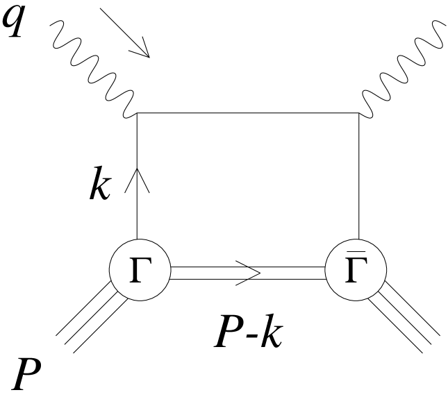
Figure 1:

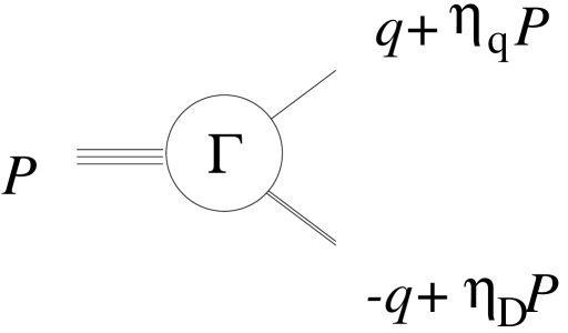
Figure 2:

Figure 3:

Figure 4:

Figure 5:

Figure 6:

References

- [1] H. Meyer and P.J. Mulders, Nucl. Phys. A528, 589 (1991); W. Melnitchouk, A.W. Schreiber and A.W. Thomas, Phys. Rev. D49, 1183 (1994); W. Melnitchouk, A.W. Schreiber and A.W. Thomas, Phys. Lett. B335, 11 (1994); W. Melnitchouk, G. Piller and A.W. Thomas, Phys. Lett. B346, 165 (1995).
- [2] K. Rothe, Phys. Rev. 170, 1548 (1968); K. Ladanyi, Nucl. Phys. B57, 221 (1973).
- [3] E. zur Linden and H. Mitter, Nuovo Cim. 61B, 389 (1969).
Figure Captions
Fig. 1: Diquark spectator process.
Fig. 2: The Bethe-Salpeter vertex function.
Fig. 3: The Bethe-Salpeter equation in the ladder approximation.
Fig. 4: The normalized radial functions and for the bound state with the mass as functions of the Euclidean momentum .
Fig. 5: The on–shell scalar functions (solid) and (dashed) as functions of the quark momentum . The mass of the bound sate is and the angular momentum is truncated at .
Fig. 6: The valence quark contributions to the structure function . The solid (dashed) line denotes the weakly (strongly) bound state with the mass: ().