LANCASTER-TH 95/07, CLNS 95/1384, SUSX-TH 96/31, hep-ph/9602263

Some aspects of thermal inflation:the finite temperature potential and topological defects

Tiago Barreiro¹, E. J. Copeland¹, David H. Lyth²

and

Tomislav Prokopec³

¹School of Mathematical and Physical Sciences,

University of Sussex, Falmer, Brighton BN1 9QH,  U. K.

²School of Physics and Chemistry, Lancaster University, Lancaster LA1 4YB,  U. K.

³Newman Lab for Nuclear Studies, Cornell University, Ithaca NY14853, USA

Abstract

Currently favoured extensions of the Standard Model typically contain ‘flaton fields’ defined as fields with large vacuum expectation values (vevs) and almost flat potentials. If a flaton field is trapped at the origin in the early universe, one expects ‘thermal inflation’ to take place before it rolls away to the true vacuum, because the finite-temperature correction to the potential will hold it at the origin until the temperature falls below $1\,\mbox{TeV}$ or so. In the first part of the paper, that expectation is confirmed by an estimate of the finite temperature corrections and of the tunneling rate to the true vacuum, paying careful attention to the validity of the approximations that are used. The second part of the paper considers topological defects which may be produced at the end of an era of thermal inflation. If the flaton fields associated with the era are GUT higgs fields, then its end corresponds to the GUT phase transition. In that case, the abundance of monopoles and of GUT higgs particles will have to be diluted by a second era of thermal inflation (or perhaps some non-thermal analogue). Such an era will not affect the cosmology of GUT strings, for which the crucial parameter is the string mass per unit length. Because of the flat Higgs potential, the GUT symmetry breaking scale required for the strings to be a candidate for the origin of large scale structure and the cmb anisotropy is about three times bigger than usual, but given the uncertainties it is still compatible with the one required by the unification of the Standard Model gauge couplings. The cosmology of textures and of global monopoles is unaffected by the flatness of the potential.

PACS: 98.80.Cq, 98.80.-k, 64.60.-i, 11.27.+d, 12.10.-g, 12.60.Jv, 14.80.Hv

1 Introduction

In presently favoured extensions of the Standard Model, the space of the scalar fields contains many directions in which the potential is almost flat out to large field values. In some of these directions the mass-squared is likely to be negative, leading to a nonzero vev whose magnitude will be large because the potential is flat. Fields of this kind, with large vevs and almost flat potentials, have been called flatons [4], and it has long been recognized that they may be cosmologically significant [5, 6, 7, 4, 8, 9, 10, 11, 12, 13].

Recently a previously almost [9] unnoticed aspect of flaton cosmology was studied, and termed thermal inflation [14, 15]. Thermal inflation is made possible by the flatness of the potential, which near the origin allows the (positive) finite temperature contribution to the mass-squared to dominate the true (negative) mass-squared long after the thermal contribution to the energy density has become negligible. If it occurs, thermal inflation completely alters the standard cosmology, and one purpose of this paper is to examine carefully the features of the finite temperature potential that are supposed to lead to it. Taking into account the validity of the various approximations, we shall verify that thermal inflation indeed takes place, provided that the field is trapped at the origin and that it has sufficiently strong interactions with light fields.

When thermal inflation ends, and the field rolls away from the origin, topological defects may be produced just as in the more familiar case of a non-flat potential. The second purpose of this paper is to see what effect the flatness of the potential has on these defects, and their cosmology. We are particularly interested in the case that the GUT higgs particles are flatons, so that the defects produced are monopoles and (depending on the GUT) cosmic strings, but we shall also study the case of global symmetry breaking.

Recently it has been pointed out [16] that the interaction of other scalar fields with the flaton might cause inflation even without thermalization. In that case the situation is more model dependent and we shall not study it in this paper, though much of our discussion of topological defects will still be applicable.

Thermal inflation is expected to take place after ordinary (slow-roll) inflation, and to last for fewer $e$-folds. Such a late epoch of inflation can play a welcome role in diluting the abundance of unwanted relics, while leaving unaltered the large-scale density perturbation accounting for the cmb anisotropy and large scale structure. (As we shall discuss this remark applies whether the perturbation is caused by a vacuum fluctuation during ordinary inflation, or by topological defects such as strings or textures.) There can be more than one epoch of thermal inflation, so that a second epoch can dilute relics left over from a first epoch, and we shall see that this is indeed essential if one is to have a GUT phase transition with a flat potential.

Before getting into more detail we need to be precise about what is meant by a ‘large’ vev, and a potential which is ‘almost flat’. In this paper we take these terms to be defined with respect to the energy scale $10^{2}$ to $10^{3}\,{\rm GeV}$, which is the scale of supersymmetry breaking as defined by the masses of the supersymmetric partners of known particles [17]. Thus the vev $M$ of a flaton field is much bigger than the above scale, whereas the the energy scale $|V^{\prime\prime}|^{1/2}$ defined by the curvature of its potential is taken to be of order that scale. In particular the mass $m$ of a flaton particle is taken to be of that order. Since the potential as well as its first derivative vanishes at the vev, its value $V_{0}$ at the origin is of order $m^{2}M^{2}$.

Each flaton is either a gauge singlet or a GUT Higgs field. A GUT is nowadays considered optional because it is difficult to implement, and can perhaps be avoided by appealing to superstring unification near the Planck scale. On the other hand the observed Standard Model couplings are compatible with the existence of a GUT, with Higgs vevs of order $10^{16}\,\mbox{GeV}$ (plus possible additional intermediate scale vevs [18]). If one accepts the existence of a GUT then it is attractive to suppose that the Higgs fields are flatons because one might then be able to understand the magnitude of the vev without inserting parameters by hand [19].

Whether or not there is a GUT, one expects to find some flatons which are gauge singlets. To understand the possibilities here, note first that each flaton will be a complex field.. If there is a single flaton field, and it is charged under a global $U(1)$ symmetry, then its vev will spontaneously break that symmetry. The prime candidate for a global $U(1)$ symmetry is the Peccei-Quinn symmetry associated with the axion, and indeed a flaton model for that symmetry has been proposed [20]. With more flaton fields one can have higher global symmetries, as we mention at the end of Section V in connection with topological defects.

However there is no need for a flaton field to be charged under a continuous symmetry; on the contrary, it is quite reasonable on the basis of current thinking to expect flaton fields which are charged under at most discrete symmetries. For them, the vacuum manifold consists of discrete points instead of an entire circle. The possibilities that we have in mind are of two kinds. The first are some or all of the moduli fields [5, 21, 22, 23, 24, 25], which are ubiquitous in versions of supergravity motivated by the superstring. For the present purpose, a modulus may be defined as a field whose potential is exactly flat in the limit of unbroken symmetry. It is widely supposed that one or more of the moduli is a flaton, with a vev of order the reduced Planck mass $m_{Pl}=(8\pi G)^{-1/2}=2.4\times 10^{18}\,{\rm GeV}$. (Lower values may be possible so that GUT Higgs fields may be moduli [19], but for simplicity, the term ‘moduli’ will be used in what follows to denote only the case where the vev is of order $m_{Pl}$. It is also possible that moduli have masses much bigger than $1\,\mbox{TeV}$, in which case they are not flatons.) Now consider the opposite possibility, of gauge-singlet flatons whose potential is not flat even in the limit of supersymmetry [15, 26]. Extensions of the Standard Model can easily contain such fields, and their potentials will resemble Eq. (4) below, with couplings perhaps or order 1. As a result, their vev is typically much smaller than the GUT scale, perhaps of order $10^{9}$ to $10^{11}\,\mbox{GeV}$.

2 Flaton cosmology

The cosmology of flatons is a rather rapidly moving research area at the moment, but we briefly summarize it here following [15, 16, 27]. For simplicity we generally pretend that there is only one flaton field $\Phi$, whose potential is invariant under a $U(1)$ symmetry so that it depends only on the magnitude $|\Phi|$. We also however point to the differences that can occur in the more realistic case, where there may be several flaton fields and a higher symmetry or else no continuous symmetry at all.

In the early universe, the effective potential of a flaton field is modified by its interaction. If the interaction with light particles is of gravitational strength, then the effective potential is expected to receive an additional contribution of order $\pm H^{2}|\Phi|^{2}$ [6, 7, 11, 28]. If it is somewhat stronger one might perhaps expect a contribution $\pm\alpha^{2}H^{2}|\Phi|^{2}$ with $\alpha$ significantly bigger than 1. One expects gravitational strength interactions for moduli with a vev of order $m_{Pl}$, whereas one expects interactions stronger by a factor perhaps $m_{Pl}/M$ for a flaton with smaller vev $M$. These statements refer to field values of order the vev, as opposed to values near the origin which we discuss in a moment, and they are based on the idea that the coupling to a light particle is suppressed by a factor $\propto 1/M$.

The weak contributions just described can be of either sign. In contrast, if the interaction is strong enough to lead to thermalization then one has the finite temperature correction to the potential, which at least near the origin gives typically a positive contribution $\sim T^{2}|\Phi|^{2}$ to the mass-squared. For a flaton field $\Phi$, one expects the thermal contribution to be present in the regime $|\Phi|\mathrel{\hbox to0.0pt{\lower 4.0pt\hbox{\hskip 1.0pt$\sim$}\hss}\raise 1.0pt\hbox{$<$}}T$ because the effective mass of particles coupling to the flaton field is of order $|\Phi|$. Section III below is devoted to a detailed study of the thermal contribution.

As a result of these modifications to the potential, a flaton in the early universe will either be at the origin or will have a value which is large but not particularly close to its true vev. We discuss these possibilities in turn.

2.1 Flaton field initially at the origin

Let us suppose that a positive effective mass-squared holds the flaton field at the origin prior to full reheating after ordinary inflation. Then the finite temperature mass-squared $\sim T^{2}$ will typically hold it there until the temperature falls to a value $T_{\mbox{\scriptsize end}}\sim m_{0}\sim 10^{2}$ to $10^{3}\,\mbox{GeV}$, where $-m_{0}^{2}$ is the true mass-squared of the flaton field at the origin. Only then will it start to oscillate about the true vev. On the other hand, the energy density with the flaton field at the origin is

$$\rho=V_{0}+\frac{\pi^{2}}{30}g_{*}T^{4}$$ (1)

where $g_{*}$ is the effective number of species. Because $T_{\mbox{\scriptsize end}}$ is so low, the first term dominates before the flaton field rolls away, leading to an era of ‘thermal’ inflation. The era starts when $T\sim V_{0}^{1/4}\sim(mM)^{1/2}$, and it ends when $T=T_{\mbox{\scriptsize end}}\sim m$, so the number of $e$-folds of thermal inflation is of order $(1/2)\ln(M/m)\sim 9+(1/2)\ln(M/10^{10}GeV)$. As a result, thermal inflation cannot replace ordinary inflation; rather, it takes place if at all after ordinary inflation has ended, at the low energy scale $V_{0}^{1/4}\sim(mM)^{1/2}\sim 10^{6}\,\mbox{GeV}(M/10^{10}\,\mbox{GeV})^{1/2}$.

After thermal inflation ends the flaton field starts to oscillate about the minimum of the effective potential, so we enter an era of matter domination by the flaton particles. (As we discuss in a moment the minimum might initially be shifted from the true vacuum, but this effect can be ignored because the movement of the minimum will be slow.) If each flaton particle decays at the single particle decay rate $\Gamma$, this era ends at the time $\Gamma^{-1}$. In typical models one estimates $\Gamma^{-1}=100\gamma^{-1}M^{2}/m^{3}$ where the numerical factor $\gamma$ is at most of order 1. At least the bulk of the decay products thermalize promptly, so setting $\Gamma^{-1}$ equal to the expansion time $H^{-1}$ where $H$ is the Hubble constant we obtain the temperature just after flaton decay to be

$$T_{\rm D}\simeq g_{*}^{-\frac{1}{4}}\Gamma^{\frac{1}{2}}m_{\rm Pl}^{\frac{1}{2}}\simeq 3\gamma^{\frac{1}{2}}\left(\frac{10^{11}\,{\rm GeV}}{M}\right)\left(\frac{m}{300\,{\rm GeV}}\right)^{\frac{3}{2}}\mbox{GeV}$$ (2)

where $g_{*}$ is the effective number of species at temperature $T_{\rm D}$, set equal to 100 for the numerical estimate.

In fact, the assumption that the flatons corresponding to the oscillation decay individually at the one-particle decay rate is not correct, because of non-linear relaxation effects of which the most studied example is parametric resonance [30, 31, 16, 32, 33, 34] (see also [35, 11]). As soon as the flaton field starts to oscillate at the end of thermal inflation, non-linear relaxation drains off a significant fraction of the oscillation, or in other words destroys a significant fraction of the corresponding flaton particles. They are replaced by marginally relativistic scalar particles of whatever species have a significant interaction with the flaton field, including the flaton field itself.

If nothing happens to the produced scalar particles they will become non-relativistic after a few Hubble times, and are expected to decay at their one-particle decay rate. If, on the other hand, they thermalize then they turn into highly relativistic radiation. At the present time it is not clear whether parametric resonance can really create particles which thermalize successfully. However, it is clear that the flaton component of the produced particles cannot thermalize because here one knows that the interaction is too weak. Furthermore, one expects that the energy density of the produced flatons will be a significant fraction of the total energy density [27]. Thus, even if the other produced particles thermalize promptly one expects that a significant fraction of non-thermalized energy will remain, and that a significant fraction of that energy will be in flaton particles.

Any thermalized radiation produced by parametric resonance will redshift away, so independently of the details one expects that a few Hubble times after the end of thermal inflation the energy density is dominated by non-relativistic scalar particles, including the flatons and perhaps other species. Each species will decay at the single-particle decay rate, so we expect eventually to find only the longest-lived species, which dominates the energy density until it decays. For simplicity we shall assume in what follows that this species is the original flaton. Then, the upshot of this discussion is that despite non-linear effects, the eventual reheat temperature is still the temperature $T_{\rm D}$ calculated from the single-particle decay rate, as given by Eq. (2).

2.2 Flaton field initially displaced from the origin

Now suppose that the flaton field has a large value in the early universe. In contrast with the first case, the field will not now be in thermal equilibrium because its interaction with light particles will be very weak (because otherwise the large value would generate a large mass for the would-be light particle). A very crude model for the evolution of the effective potential of a flaton field $\Phi$ in the early universe is [15, 27, 36]

$$V(|\Phi|)=m^{2}(|\Phi|-M)^{2}+\alpha H^{2}(|\Phi|-\Phi_{0})^{2}$$ (3)

where $M$ is the true vev. The second term represents the effect of interactions in the early universe, and for the present purpose we can suppose that $\Phi_{0}\sim M$ is a constant, so that the only time dependence comes from $H$.

First suppose that $\alpha$ is of order 1, which is the expected value at least for a flaton such as a modulus with gravitational strength interactions (corresponding to $M\sim m_{Pl}$). In that case [15], the minimum of $V$ is practically at $\Phi_{0}$ until the epoch $H\sim m$, after which it moves quickly to the true vev $M$. The flaton will have settled down to the minimum of $V$ before the end of ordinary inflation, so the conclusion is that if $\alpha$ is of order 1 the flaton field starts oscillating about the true vev at the epoch $H\sim m$, with initial amplitude $|\Phi_{0}-M|\sim M$.

As soon as the oscillations start, non-linear relaxation effects will convert a significant fraction of the energy in the oscillating flaton field. Provided that the oscillation continues to take place about the true vev, then the qualitative picture will not be altered, just as we discussed already in the case of an oscillation starting out at the origin. However, because the initial oscillation energy can now be bigger than the potential energy $V_{0}$ at the origin, there is now the possibility that non-linear relaxation effects restore the symmetry, so that the oscillation takes place about the origin [16]. In that case the flaton field oscillation might give way to some $e$-folds of inflation, which might be thermal inflation, before the symmetry breaks [16]. If it occurs, this will happen when the energy density is equal to $V_{0}\sim(mM)^{2}$, which is much less than the energy density $\rho\sim(mm_{Pl})^{2}$ at the epoch when the oscillation starts.

Finally, consider the case $\alpha\gg 1$. The evolution of the flaton field is now quite different [27], because the movement of the minimum of the effective potential is always slow on the timescale of oscillations around it. As a result the flaton is at all times close to the minimum of its effective potential, and the cosmological production of flaton fields is strongly suppressed. (To be precise, analytic [36] and numerical [27] estimates show that the amplitude of the oscillation about the minimum is reduced exponentially compared with the case $\alpha\sim 1$.)

2.3 The case of more than one flaton field

So far we have considered only a single flaton species. If there are several, then some may be initially trapped at the origin and some may be displaced from it. Those which are displaced start to oscillate first (when the energy density is $\rho\sim(mm_{Pl})^{2}$, corresponding to a Hubble parameter $H\sim m$), while those trapped at the origin give rise to thermal inflation. If several flaton fields are trapped at the origin, the simplest possibility is that they all roll away at more or less the same epoch, which seems reasonable because the negative mass-squared is of the same order for all flatons, and so is the finite-temperature correction. If that happens, we essentially recover the case of a single flaton. However, the rolling away of the first flaton (say) might trap the remaining flatons at the origin through its interactions. One possibility is that the particles produced by non-linear relaxation promptly thermalize, in which case one may enter a second era of thermal inflation [15]. Alternatively the remaining flatons may be trapped by non-linear relaxation [16], which could also lead to a second epoch of inflation.

In this paper, we are assuming for simplicity that only genuine flatons can roll away from the origin. It could happen that a field with a flat potential, and zero true vev, couples to a flaton in such a way that its effective potential acquires a nonzero minimum by virtue of the zero value of this flaton. Such a field could temporarily act as a flaton, leading to a more complicated cosmology [26] which we shall not consider.

2.4 The entropy crisis and its solutions

If a flaton comes to dominate the energy density of the universe, then the low ‘reheat’ temperature Eq. (2) makes it cosmologically fatal if its vev is too large. Indeed, successful nucleosynthesis requires $T_{\mbox{\scriptsize D}}\mathrel{\hbox to0.0pt{\lower 4.0pt\hbox{\hskip 1.0pt$\sim$}\hss}\raise 1.0pt\hbox{$>$}}10\,\mbox{MeV}$, corresponding to $M\mathrel{\hbox to0.0pt{\lower 4.0pt\hbox{\hskip 1.0pt$\sim$}\hss}\raise 1.0pt\hbox{$<$}}10^{14}\,{\rm GeV}$, and thermalization of a stable LSP requires $T_{\mbox{\scriptsize D}}\mathrel{\hbox to0.0pt{\lower 4.0pt\hbox{\hskip 1.0pt$\sim$}\hss}\raise 1.0pt\hbox{$>$}}1\,\mbox{GeV}$ corresponding to $M\mathrel{\hbox to0.0pt{\lower 4.0pt\hbox{\hskip 1.0pt$\sim$}\hss}\raise 1.0pt\hbox{$<$}}10^{12}\,{\rm GeV}$. (To have electroweak baryogenesis requires $T_{\mbox{\scriptsize D}}\mathrel{\hbox to0.0pt{\lower 4.0pt\hbox{\hskip 1.0pt$\sim$}\hss}\raise 1.0pt\hbox{$>$}}100\,\mbox{GeV}$ corresponding to $M\mathrel{\hbox to0.0pt{\lower 4.0pt\hbox{\hskip 1.0pt$\sim$}\hss}\raise 1.0pt\hbox{$<$}}10^{10}\,{\rm GeV}$, but this requirement is not mandatory especially as thermal inflation itself provides additional possibilities for baryogenesis [16, 26].)

This possible problem is a concern for any moduli which are flatons with a vev $M\sim m_{Pl}$, and it is also a concern for GUT Higgs fields if they are flatons since the corresponding vev is $M\sim 10^{16}\,\mbox{GeV}$. It was originally termed the ‘entropy crisis’ [5], and was widely discussed in the 1980’s [6, 7, 8, 9, 10, 11, 12, 13]. More recently, focusing on moduli, it has been termed the moduli problem [21, 22, 23, 24, 25].

Let us consider the status of the ‘moduli’ problem, in the light of the above snapshot of the current status of flaton cosmology. First, it should be emphasised that the problem exists only if the fields in question are actually flatons, with masses $\sim 10^{2}$ to $10^{3}\,\mbox{GeV}$. Assuming that this is the case, the status of the problem depends on whether or not the flaton in question is initially displaced from the origin. If it is, the problem may not occur at all, because the flaton may settle down smoothly to the true vacuum without appreciable oscillations; this may well occur for the GUT Higgs though it is less likely for the moduli [27, 36]. If it does occur it can be solved by a subsequent bout of thermal inflation, associated with a flaton having a cosmologically safe vev $M\mathrel{\hbox to0.0pt{\lower 4.0pt\hbox{\hskip 1.0pt$\sim$}\hss}\raise 1.0pt\hbox{$<$}}10^{12}\,\mbox{GeV}$. As we remarked earlier, typical extensions of the Standard Model indeed contain such flatons.

If, on the other hand, the flaton in question is initially at the origin, then thermal inflation will occur and when it ends the flaton will certainly oscillate with large amplitude. In that case one needs a second era of thermal inflation [15], again associated with some other flaton which has a cosmologically safe vev. At least naively this in turn requires prompt thermalization of a significant fraction of the original flaton oscillation energy (with non-linear relaxation presumably first converting the energy into marginally relativistic particles) and at the present time it is not clear whether this is possible. If it is not possible, then we reach the important conclusion that flatons with dangerously large vevs, like moduli and GUT Higgs fields, cannot be associated with thermal inflation. We return to this issue for GUT Higgs fields in Section V.

3 The 1-loop thermal effective potential

In this section and the following one, we examine carefully the finite temperature effects that are supposed to make thermal inflation possible. They were first described by Yamamoto in 1986 [8], but his account was brief and it did not discuss the validity of the various approximations employed. To our knowledge no subsequent authors have improved on Yamamoto’s discussion.

As already remarked, the potential of the relevant flaton fields might be invariant under a continuous symmetry such as a global $U(1)$ or a GUT gauge symmetry, or alternatively it might have no continuous symmetry. The computations in this paper will be applied to a simple toy model, in which there is a single flaton field with a $U(1)$ symmetry. Following [14, 15], we take the potential to be of the form

$$V=V_{0}-m_{0}^{2}\Phi^{\dagger}\Phi+\frac{\lambda_{n}}{m_{Pl}^{2n}}\left(\Phi^{\dagger}\Phi\right)^{n+2}$$ (4)

where $n$ is an integer power. Here $m_{0}$ is of order $10^{3}\,\mbox{GeV}$, and for simplicity we have included only the leading non-renormalizable term. The magnitude of the coupling $\lambda_{n}$ is model dependent, but for definiteness one can keep in mind a value of order $1$. We can parametrize the quantum field $\Phi$ as follows:

$$\Phi=\frac{\phi}{\sqrt{2}}+\delta\phi+i\eta,$$ (5)

where $\phi$ is the classical degree of freedom, which equals to the expectation value of $\sqrt{2}\langle\Phi\rangle$, and $\delta\phi$ and $\eta$ are quantum fluctuating fields with zero expectation values. The classical part of the effective potential can be then written as

$$V=V_{0}-\frac{1}{2}m_{0}^{2}\phi^{2}+\frac{\lambda_{n}}{m_{Pl}^{2n}}\left(\frac{\phi^{2}}{2}\right)^{n+2}$$ (6)

From this expression we can easily obtain the mass $m_{\phi}$ of the flaton particle given by $m^{2}_{\phi}=d^{2}V/d\phi^{2}(\phi=\sqrt{2}M)$, the vacuum expectation value $M=\langle\Phi\rangle_{0}$, corresponding to the minimum of $V$, and the height $V_{0}$ of the potential at the origin which one gets by setting $V(M)=0$. The result is

$$m^{2}_{\phi} = 2(n+1)m_{0}^{2}$$ (7)

$$M^{2(n+1)} = \frac{1}{\lambda_{n}}\frac{1}{n+2}\;m_{Pl}^{2n}\;\;m_{0}^{2}$$ (8)

$$V_{0} = \frac{n+1}{n+2}\;M^{2}\,m_{0}^{2}$$ (9)

One naively expects $\lambda_{n}\sim 1$ ($n\geq 1)$ for the couplings, making $M\sim 10^{10}\,\mbox{GeV}$. On the other hand, it might be that the Planck scale is replaced by the GUT scale if there is one, which effectively increases $\lambda_{n}$ leading [15] to $M\sim 10^{9}$. Finally, $\lambda_{n}$ might be a small mass ratio, which could make $M\gg 10^{10}$ so that it becomes [15] the GUT scale (appropriate if $\phi$ is a GUT Higgs field) or the Planck scale (appropriate if $\phi$ is a modulus). In this paper we focus on the first and second cases.

3.1 Coupling to bosons

Now consider the finite-temperature correction to the effective potential. First we will argue that the thermal correction from the $\Phi$ field itself is irrelevant in the sense that it can neither trap the field at the origin nor cause a phase transition. Then, in order to cure this we will assume either that $\Phi$ couples to another (real) scalar field via a quartic coupling of form $g\Phi^{\dagger}\Phi\chi^{2}$, or gauge the U(1) by adding the corresponding gauge field. We shall also consider the effect of coupling to a spin-half field since we have in mind the case of supersymmetry.

The one-loop thermal correction of a bosonic excitation with the mass $m$ to the effective potential has the following generic form [37]

$$V_{1}(m,T)=\frac{T^{4}}{2\pi^{2}}\int_{0}^{\infty}dxx^{2}\ln\left(1-e^{-\sqrt{x^{2}+m^{2}/T^{2}}}\right)$$ (10)

Below we will always quote a one loop result for $m$. One should keep in mind that strictly speaking in order to obtain the one loop thermal correction to the effective potential from Eq. (10) one should use the tree level value for $m$. In some cases the ring-improved one loop potential (which is a result of resumming certain so-called ring diagrams to all orders) is more accurate. It corresponds to using the one-loop thermal value for the effective mass only for the ‘singular’ term $-m^{3}T/12\pi$ in the high temperature expansion.

The one-loop value for the masses follow: $m_{\phi}^{2}\simeq-m_{0}^{2}+gT^{2}/12$ is the mass-squared of the $\Phi$-field excitations, and $m_{\chi}^{2}=m_{\chi}^{2}(T=0)+gT^{2}/12+g\phi^{2}$ is the mass-squared of $\chi$. Note that in this approximation $m_{\phi}$ does not acquire a $\phi$-dependent correction. Indeed, the lowest order correction to $m_{\phi}^{2}$ proportional to $\phi^{2}$ occurs at the $(n+1)$-loop level and is of order $\lambda_{n}T^{2}(T/m_{Pl})^{2n}$, which is minute and hence negligible. We now see from Eq. (10) that the finite temperature contribution due to the $\Phi$ field excitations is to an excellent approximation a $\Phi$-independent shift in the effective potential. This shift is nothing but adding a constant to the energy density and hence it should not affect the dynamics of the $\Phi$ field.

The complete effective potential is now $V(\phi,T)=V(\phi)+\sum_{i}V_{1}(m_{i},T)$, where we are summing over all the boson fields. In the regime $m_{i}\simeq\sqrt{g}\phi>>T$, the finite temperature correction $V_{1}$ is negligible. (As we remarked earlier, one does not in any case expect thermalization in this regime, since particles with mass $m\ll\phi$ must couple weakly to $\phi$ [15].) In the opposite regime $m_{i}\simeq\sqrt{g}\phi\ll T$, the correction is $V_{1}\simeq-T^{4}\zeta_{4}/\pi^{2}$ with $\zeta_{4}=\pi^{4}/90$, which is independent of $\phi$. The conclusion is that at large temperatures $T\gg M$, the potential has a single minimum at $\phi=0$. (Recall that $M$ is the position of the true vacuum, defined by Eq. (8).) As the temperature drops a second minimum develops. At a critical temperature $T_{c}$ defined by $V(T_{c},\phi=0)=V(T_{c},\phi=\sqrt{2}M)$ the two minima are degenerate. This temperature is given by

$$T_{c} = \left(\frac{n+1}{n+2}\frac{\pi^{2}}{\zeta_{4}}\right)^{1/4}(Mm_{0})^{1/2}\sim V_{0}^{1/4}$$ (11)

The bump in the effective potential which causes the phase transition is solely due to the $\chi$ field excitations. Even though there are two degenerate minima the field will be trapped at $\phi=0$, i.e. there will be no phase coexistence since the bump is very large and the tunneling rate is minute, much smaller than the expansion rate of the Universe. A large bump at the critical temperature indicates that the phase transition is strongly first order. As the Universe cools down below $T_{c}$, trapped in the false vacuum phase $\phi=0$, the false vacuum energy starts dominating. Using Eq. (1), this occurs at the temperature $T_{TI}^{4}\simeq V_{0}\pi^{2}/3g_{*}\zeta_{4}$, at which Thermal Inflation begins. The effective number of particle species $g_{*}$ is equal 3 in our toy model, two from the $\phi$ field and one from the $\chi$-field. In general $g_{*}$ will be of order $10^{2}-10^{3}$. Note that, according to the rough estimate Eq. (1), the temperature $T_{c}$ is of the same order of magnitude as the temperature $T_{TI}$ at which thermal inflation begins.

Thermal inflation ends when the Universe supercools sufficiently so that the tunneling rate for creation of the true vacuum bubbles becomes comparable to the expansion rate of the Universe. We will postpone a more detailed study of the bubble nucleation to the next section.

So far we have focussed on the coupling to a spin zero particle $\chi$. If the flaton is a GUT Higgs field there will also be a coupling to gauge particles. As a toy model, consider the Abelian Higgs model, whose Lagrangian density is ${\cal L}=-F^{\mu\nu}F_{\mu\nu}/4+(D_{\mu}\Phi)^{\dagger}(D^{\mu}\Phi)-V$, where $D_{\mu}=\partial_{\mu}+ieA_{\mu}$, $A_{\mu}$ is the vector field, and $F^{\mu\nu}$ is the field strength. The thermal correction to the potential has again the form of Eq. (10) but with the masses squared $m^{2}_{\phi}=-m_{0}^{2}+(3e^{2})T^{2}/12$ for both the physical excitation and the unphysical Goldstone boson of the $\phi$-field, and $m_{L}^{2}=e^{2}\phi^{2}+(e^{2}/3)T^{2}$, $m_{T}^{2}=e^{2}\phi^{2}$ for (one) longitudinal and (two) transverse polarized gauge field excitations, respectively. At this level some gauge dependence may come into the play, but we will not discuss this issue here. The above analysis caries through in almost exactly the same way, except that the masses in the thermal potential are now $m_{L}$, $m_{T}$ and $m_{\phi}$. There are 5 degrees of freedom relevant for the onset of thermal inflation, so the temperature at which it begins will be somewhat lower, as will be the critical temperature.

What about the validity of the one-loop approximation? The squared coupling of the three dimensional theory is $g_{3}^{2}=gT$ for a scalar theory and $g_{3}^{2}=e^{2}T$ for a gauged theory. Each loop added costs an extra factor $gT/M$; recall that $M_{\chi}\simeq\sqrt{g}\phi$, $M_{T,L}\simeq e\phi$, so that we expect the one-loop approximation to break down when $g_{3}^{2}>M$, which means $\phi/T<\sqrt{g}$ for the scalar theory and $\phi/T<e$ for the gauge theory. In other words, the one-loop approximation can be trusted as one approaches the critical temperature up to $|T-T_{c}|\sim gT,\;e^{2}T$. In this case, unlike in the case of the electroweak theory, the one-loop treatment is accurate. The reason is that the maximum of the effective potential (bump) is located at

$$\phi_{1}\sim\frac{T}{\sqrt{g}}$$ (12)

This should be taken only as an estimate since the bump is located where neither the high temperature nor the low temperature expansion is accurate. Nevertheless, this estimate tells us something important about the validity of the one loop approximation: the bump is located in the region of validity of the one-loop approximation (this is, for example, not true in the electroweak theory); it is $1/g$ times larger for the scalar theory ($1/e^{2}$ for the gauge theory) than the value of $\phi$ at which we expect the breakdown of the one-loop approximation. We see that, at the local maximum, the 1-loop potential is still a reasonable approximation to the true effective potential and this treatment of the phase transition is quite accurate. One can also evaluate the potential energy density at the bump. To get a feeling for what it is we evaluate it in the high temperature limit and find $V(\phi_{1})\sim V_{0}-T^{4}\pi^{2}(1/90-1/648)$. Hence we see that the energy density of the bump $(T^{4}\pi^{2}/648)$ is much smaller than the energy density difference between the false and true vacua $(V_{0}-T^{4}\pi^{2}/90)$. This suggests that the wall of the critical bubble is thick, which will be used in the following section where we study nucleation.

3.2 Coupling to fermions

To illustrate what happens in the case of a scalar field coupling with fermions, we include in the global U(1) potential a Yukawa coupling of the scalar to a spinor field $y_{f}\phi\bar{\psi}\psi$. We will then have a contribution to the effective potential of the form

$$V_{1}^{f}(m_{f},T)=-\frac{T^{4}}{2\pi^{2}}\int_{0}^{\infty}dxx^{2}\ln\left(1+e^{-\sqrt{x^{2}+m^{2}_{f}/T^{2}}}\right)$$ (13)

where the fermion mass is $m_{f}(\phi)=y_{f}\phi$. This yields a critical temperature very close to the scalar coupling case of Eq. (11) with a minor numerical difference: since each fermion contributes to the free energy $7/8$ times less than a boson, with the same number of degrees of freedom, $T_{c}$ will be higher by a factor $(8/7)^{1/4}$. The local maximum $\phi_{1}$ will also be the same (replacing $e$ by $y_{f}$). One should note an important difference between this phase transition and the electroweak phase transition. Since the main reason for the free energy valley at around $\phi\sim 0$ is not the singular cubic term $-m_{f}^{3}T/12\pi$ in the high temperature expansion of Eq. (10), but the exponential suppression of the population density for the mass $m_{f}>>T$, the only difference in studying the cases of coupling to bosons and fermions is the trivial one of counting degrees of freedom. The total effective number of degrees of freedom is $g_{*}({\rm tot})=\frac{7}{8}g_{*}({\rm fermion})+g_{*}({\rm boson})$. This remark will be also valid when studying the nucleation problem in the next section.

4 Tunneling

We are taking the standard route as advocated by Callan, Coleman [38], and Linde [39] in which we assume that the spherical three dimensional action

$$S_{3}=\int d^{3}r\left[{1\over 2}(\nabla\phi)^{2}+V(\phi,T)\right]$$ (14)

determines the nucleation rate per unit time and volume

$$\frac{\Gamma}{V}=m^{4}\left(\frac{S_{3}}{\pi T}\right)^{3/2}{\rm e}^{-S_{3}/T}\,,\qquad m^{2}=m_{\chi}^{2}\simeq\frac{gT^{2}}{12}+g\phi^{2}$$ (15)

This is an approximate formula but it is sufficiently accurate for our purposes. A more accurate treatment of bubble nucleation can be find in [40]. The rate in Eq. (15) has to be compared with the expansion rate of the Universe to determine the rate of bubble formation. More precisely [41], assuming a constant bubble expansion velocity, at any given time the fraction of the Universe remaining in the symmetric phase is given by

$$\exp\left(-\int_{-\infty}^{t}\frac{4\pi}{3}v^{3}(t-t^{\prime})^{3}\frac{\Gamma}{V}\,dt^{\prime}\right)$$ (16)

In order to solve for the nucleation temperature we expand $S_{3}$ about the value when the integrand is about one: $S_{3}=S_{3}(T_{nucl})+(t-t^{\prime})(dS_{3}/dt)$, where $d/dt=(dT/dt)d/dT$, $dT/dt=-TH$, and $H^{2}=(8\pi G/3)(\pi^{2}g_{*}(T)T^{4}/30)$ is the Hubble constant. Using a saddle point approximation we find that the integral is of order one when

$${\rm e}^{S_{3}(T_{nucl})/T_{nucl}}=\frac{8\pi v^{3}}{(HdS_{3}/dT)^{4}}m^{4}\left(\frac{S_{3}(T_{nucl})}{\pi T_{nucl}}\right)^{3/2}$$ (17)

In order to solve this equation we have to find what is the bubble action $S_{3}$ as a function of temperature.

The solution to the (spherically symmetric, classical) equation of motion for $\phi$:

$${d^{2}\over dr^{2}}\phi+{2\over r}{d\over dr}\phi={d\over d\phi}V(\phi,T)$$ (18)

with the boundary conditions:

$$\frac{d\phi}{dr}|_{r=0}=0\,,\qquad\phi(r\rightarrow\infty)=0$$ (19)

specifies the wall profile. The bubble action is

$$S_{3}=4\pi\int r^{2}\,dr\left[\left(\frac{d\phi}{dr}\right)^{2}+V(\phi,T)-V(0,T)\right]$$ (20)

Since Eq. (18) is analytically intractable, various approximation schemes have been developed. In general when the height of the local maximum is small (large) in comparison to the false vacuum energy, the thick (thin) bubble wall approximation gives a reasonably accurate answer to $S_{3}$. First one can show using the thin wall approximation, which is accurate around $T_{c}$, that the three dimensional action: $S_{3}\sim(2\pi/3)\sigma^{3}/V(0,T)^{2}$ is indeed huge; here $\sigma=\int_{0}^{\phi;V(\phi,T)-V(0,T)=0}\sqrt{2[V(\phi,T)-V(0,T)]}d\phi\sim T_{c}^{3}/\sqrt{g}$ is the surface tension of the bubble, and near the critical temperature $V(0,T)=\frac{\zeta_{4}}{\pi^{2}}(T_{c}^{4}-T^{4})<<T_{c}^{4}$.

When the temperature drops significantly below $T_{c}$, such that $V_{\rm bump}<<V(0,T)$, where $V_{\rm bump}$ is the difference between the maximum of the potential and $V(0,T)$, the thick wall approximation becomes appropriate. Here we present a heuristic discussion. The three dimensional action for the critical bubble can be approximated as follows:

$$S_{3} \sim 2\pi R_{c}\phi^{2}-\frac{4\pi}{3}R_{c}^{3}\left[V(0,T)-V(\phi,T)\right]$$ (21)

$$V(0,T)-V(\phi,T) \simeq \frac{1}{2}\frac{m_{0}^{2}T^{2}}{g}\varphi^{2}+T^{4}\left(\frac{\varphi}{2\pi}\right)^{3/2}\,{\rm e}^{-\varphi}-T^{4}\frac{\zeta_{4}}{\pi^{2}}\,,\qquad\varphi=\frac{\sqrt{g}\phi}{T}$$ (22)

where $\phi$ is the field value at the centre of the bubble. The critical action is extremal with respect to $R$ and $\phi$:

$$\frac{\partial S_{3}}{\partial R_{c}}=0\,,\qquad\frac{\partial S_{3}}{\partial\phi_{c}}=0$$ (23)

The first condition gives for the size of the critical bubble and the action:

$$R_{c}^{2}\simeq\frac{\phi^{2}}{2\left[V(0,T)-V(\phi,T)\right]}\,,\qquad S_{3}\simeq\frac{4\pi}{3}\frac{\phi^{3}}{\sqrt{2\left[V(0,T)-V(\phi,T)\right]}}$$ (24)

which can be re-written as

$$S_{3}\sim\frac{4\pi}{3g}\frac{T^{2}}{m_{0}}\frac{\varphi^{3}}{\sqrt{\varphi^{2}-2(\sqrt{g}T/m_{0})^{2}(\zeta_{4}/\pi^{2})+2(\sqrt{g}T/m_{0})^{2}(\varphi/2\pi)^{3/2}\exp-\varphi}}$$ (25)

The variation of $S_{3}$ with respect to $\varphi$ gives then the value of $\varphi$ at the origin of the bubble:

$$\varphi^{2}\simeq\frac{3\zeta_{4}}{\pi^{2}}\left(\frac{\sqrt{g}T}{m_{0}}\right)^{2}$$ (26)

which is obtained by neglecting the exponentially small term in Eq. (25) so that the critical action is

$$s_{3}=\frac{S_{3}}{T}\simeq\frac{4\sqrt{3}\zeta_{4}}{\pi}\left(\frac{T}{m_{0}}\right)^{3}$$ (27)

We can now use this result and Eq. (16) – (17) to obtain the nucleation temperature $T_{nucl}$:

$$s_{nucl}\equiv\frac{S_{3}(T_{nucl})}{T_{nucl}}\simeq-6+4\ln\frac{m_{Pl}}{M}+\frac{1}{6}\ln\frac{S_{3}}{T}\simeq 17+4\ln\frac{10^{16}GeV}{M}$$ (28)

where we assumed that the bubble is supersonic: $v\sim 1$; this is plausible since supercooling is very large. temperature is about $T_{nucl}\simeq 2m_{0}$. For somewhat different values of parameters $T_{nucl}$ changes only slightly. To a very good approximation $T_{nucl}$ is proportional to $m_{0}$. (Here we have neglected a logarithmic dependence of the form $(\ln m_{0})^{1/3}$.)

These results are in substantial agreement with that of Yamamoto [8], who found that the bubble action is (up to $\ln m_{0}$) proportional to $T^{4}/m_{0}^{3}$. What we have done is to look more carefully at the somewhat delicate assumptions which have to be made in order to derive it. We have found that at a reasonable level of confidence they can indeed be justified by carefully considering the regime of validity of the various approximations.

5 Topological defects with a flat potential

Now we come to the second part of our investigation, which is to look at topological defects associated with a flat potential. In the case of a single (complex) flaton field with a $U(1)$ symmetry, which we have focussed on for the sake of simplicity, these are cosmic strings. If instead there is only a discrete $Z_{n}$ symmetry they are domain walls. Finally, if there are two or more flaton fields there could be a higher continuous symmetry, which, depending on the pattern of symmetry breaking, could lead to monopoles and/or textures (or to no defects at all). We shall consider all these cases.

In order for the defects to form, the symmetry has to be restored at early times, which as discussed in Section 2 may or may not happen for a given flaton field. Assuming that it is indeed restored the defects form when the field rolls away from the origin, and since we are considering a flaton field this occurs at the end of an era of thermal inflation. Thus, we are considering the formation of topological defects at the end of such an era.

We shall focus particularly on the case where there is a GUT whose Higgs fields have a flat potential, schematically of the form Eq. (4). As mentioned already such a flat potential seems quite natural, because one can then hope to generate the required vev from scales already present in the theory [19]. For example, in Eq. (4), the coupling $\lambda_{n}$ might be of the form $(m_{\tilde{g}}/m_{Pl})^{p}$, where $m_{\tilde{g}}$ is related to vevs arising from gaugino condensation, and $p$ is a positive integer. This paradigm is of course very different from the usual one, where the potential of the GUT Higgs is supposed to be non-flat so that it has the form

$$V=\lambda(\Phi^{\dagger}\Phi-M^{2})^{2}$$ (29)

with $\lambda\sim 1$. Such a form is indeed natural for the Standard Model Higgs where $M$ is only of order the susy breaking scale $10^{2}$ to $10^{3}\,\mbox{GeV}$, but it seems far less natural for a GUT. In other words, there seems to be no reason to suppose that the vev of a GUT Higgs is of the same order of magnitude as its mass.

GUT symmetry breaking with a flat potential is completely different from the usually considered case. The GUT phase-transition occurs at the end of an era of thermal inflation. Just before it occurs, the potential energy density $V_{0}$ of the Higgs field accounts for most of the energy density in the universe, and after the transition this energy is initially converted into a homogeneous oscillation of the Higgs field (away from any topological defects), corresponding to extremely non-relativistic Higgs particles. Through non-linear relaxation effects this initial era is quickly followed by one in which at least a significant fraction of the energy density resides in marginally relativistic scalar particles, of various species including the Higgs particles. There may also be a significant fraction in thermalized (and hence highly relativistic) particles, but this question has not been settled at the present time.

Because the potential is flat, the GUT Higgs particles are light (mass $m\sim 10^{2}$ to $10^{3}\,\mbox{GeV}$), and according to Eq. (2) they decay after nucleosynthesis. In order not to upset nucleosynthesis their abundance must be diluted by a second era of thermal inflation. Such an era requires the thermalization of a substantial fraction of the Higgs particles, and, taking the fraction to be of order 1, but not very close to it, the abundance of the Higgs particles immediately after thermalization is $n/s\sim V_{0}^{1/4}/(g_{*}^{1/4}m)\sim 10^{6}$. From [42], their abundance at the epoch of nucleosynthesis must satisfy $n/s\mathrel{\hbox to0.0pt{\lower 4.0pt\hbox{\hskip 1.0pt$\sim$}\hss}\raise 1.0pt\hbox{$<$}}10^{-12}$, so the second bout of thermal inflation should dilute the abundance by a factor of at least $10^{18}$.

The actual dilution factor actually provided by thermal inflation is [15]

$$\Delta\sim\frac{\epsilon}{75}\frac{m^{2}M^{2}}{T_{\mbox{\scriptsize D}}T_{\mbox{\scriptsize end}}^{3}}\sim 10^{18}\left(\frac{M}{10^{11}\,\mbox{GeV}}\right)^{2}\left(\frac{1\,\mbox{GeV}}{T_{\mbox{\scriptsize D}}}\right)$$ (30)

In this expression $m$ and $M$ refer to the second era of thermal inflation, as do $T_{\mbox{\scriptsize end}}$ (the temperature at the end of thermal inflation) and $T_{D}$ (the reheat temperature). The quantity $\epsilon\leq 1$ is the fraction of energy left unthermalized after non-linear relaxation effects have occurred after the end of the second bout of thermal inflation, which we set equal to 1.

In making the above estimates we have set $V_{0}=m^{2}M^{2}$ and $T_{\mbox{\scriptsize end}}=m=10^{2.5}\,\mbox{GeV}$ for both eras of thermal inflation. The expected range for the vev of the inflaton causing the second bout of thermal inflation is $10^{9}\,\mbox{GeV}\mathrel{\hbox to0.0pt{\lower 4.0pt\hbox{\hskip 1.0pt$\sim$}\hss}\raise 1.0pt\hbox{$<$}}M\mathrel{\hbox to0.0pt{\lower 4.0pt\hbox{\hskip 1.0pt$\sim$}\hss}\raise 1.0pt\hbox{$<$}}10^{12}\,\mbox{GeV}$ (with the lower limit coming from the discussion after Eq. (8) and the upper limit from the requirement of decay before nucleosynthesis). Since several parameters have been set equal to fiducial values, a second bout of thermal inflation seems well able to provide the necessary dilution. The only problem is to ensure that it occurs, bearing in mind the fact mentioned earlier that the possibility of thermalization immediately after thermal inflation ends has not been demonstrated.

Assuming that the GUT particles can be somehow diluted, we proceed to a discussion of the defects produced, starting with monopoles.

5.1 Monopoles

It is well known that monopoles form when the vacuum manifold $M$ of a gauge group $G$ contains non-shrinkable 2 surfaces, i. e. when $\pi_{2}({\rm M})\neq I$, where $\pi_{2}$ is the second homotopy group. In the light of a theorem in homotopy theory, this may be rephrased as: monopoles form whenever a grand unified semisimple group $G$ breaks down to a group H which has nontrivial fundamental homotopy group $\pi_{1}({\rm H})\neq I$, i.e. H contains non-contractable loops. A simple example is an H which contains at least one U(1) as a factor, just like the Standard Model! It is argued in [43] that since supersymmetry does not change the connected structure of the (super)-Lie group, the same consideration as above is valid for a supersymmetric GUT. Since rather generically the symmetry of a low energy theory contains non-contractable loops, one must check what would be the cosmological implications of monopoles’ formation, i.e. whether there is a monopole problem.

It is convenient to specify the monopole abundance $n_{mon}$ as a fraction of the entropy density $s$, because $n_{mon}/s$ is constant as long as monopoles are not destroyed, except when particle decay (or some other non-equilibrium process) increases the entropy per comoving volume. Consider first the observational upper bound on the present monopole abundance. The mass of a gauge monopole for a given vev $M$ is not much affected by the flatness of the potential, because it is known that the mass goes to a finite limit as the potential becomes flatter and flatter (Bogomolny bound) [44]. This leads to a simple and reliable bound on the present monopole abundance of $n_{mon}/s\mathrel{\hbox to0.0pt{\lower 4.0pt\hbox{\hskip 1.0pt$\sim$}\hss}\raise 1.0pt\hbox{$<$}}10^{-24}$, coming from the requirement that the monopole density be less than critical. This bound is stronger than that derived from the requirement that monopoles do not affect nucleosynthesis. The next bound one can derive is based on the requirement that the galactic magnetic field not be dissipated through acceleration of monopoles from the time of galaxy formation [45]. Strictly speaking this bound applies only to the monopole abundance in galaxies. The original Parker bound is $n_{mon}/s\mathrel{\hbox to0.0pt{\lower 4.0pt\hbox{\hskip 1.0pt$\sim$}\hss}\raise 1.0pt\hbox{$<$}}10^{-24}$. This was argued to be too strong; when the depletion of monopoles, as they get accelerated and ejected from the galaxy, is taken into account [46], the bound becomes $n_{mon}/s\mathrel{\hbox to0.0pt{\lower 4.0pt\hbox{\hskip 1.0pt$\sim$}\hss}\raise 1.0pt\hbox{$<$}}10^{-20}$. A stronger bound was found using the fact that a grand unified monopole catalyzes nucleon decay [47], when captured by a neutron star; the bound is $n_{mon}/s\mathrel{\hbox to0.0pt{\lower 4.0pt\hbox{\hskip 1.0pt$\sim$}\hss}\raise 1.0pt\hbox{$<$}}10^{-30}$ [48]. A more stringent bound can be derived based on monopole capture and consequent catalytic nucleon decays in the main sequence stars [44]: $n_{mon}/s\mathrel{\hbox to0.0pt{\lower 4.0pt\hbox{\hskip 1.0pt$\sim$}\hss}\raise 1.0pt\hbox{$<$}}10^{-36}$. The flatness of the potential is not expected to alter this bound because the strong interaction cross section for the monopole is independent of its radius [47, 49].

In order to find out whether there is a monopole problem, we ought to compare the above bounds with the amount of monopoles that form at the phase transition. Since we need a second epoch of thermal inflation (to dilute the GUT Higgs particles), a significant fraction of the energy density had better thermalize immediately after the GUT Higgs phase transition, leading to a temperature $T_{\mbox{\scriptsize GUT}}\sim(mM)^{1/2}\sim 10^{9}\,\mbox{GeV}$. (Here $m\sim 10^{2}$ to $10^{3}\,\mbox{GeV}$ is the mass of a typical GUT Higgs particle with a flat potential, and $M\sim 10^{16}\,\mbox{GeV}$ is the vev of a typical GUT Higgs field.) This is much bigger than the temperature $T\sim m$ just before thermalization, but it is still far below the temperature $T\sim M$ which one would obtain after thermalization with a non-flat potential. In the case of a non-flat potential the temperature is high enough to initially annihilate the monopoles, so that when annihilation ceases there is of order one monopole per horizon volume irrespective of the initial abundance. For a flat potential this is not the case, and we have to consider the initial abundance.

A lower limit on it is provided by the causality bound which states that on average about $p\simeq 1/8$ monopoles form per causality volume $V_{c}\simeq(4\pi/3)H^{-3}$, where $H^{-1}$ is the causality radius. The probability $p\simeq 1/8$ can be obtained from an argument based on the Kibble mechanism: the field is uncorrelated on superhorizon scales, and the probability that the randomly oriented field in different correlation volumes will cover more than half of the vacuum manifold is about $p=1/8$. This bound gives an initial monopole density $n_{mon}\simeq(3/4\pi)pH^{3}$, corresponding to

$$\left(\frac{n_{mon}}{s}\right)_{caus}\mathrel{\hbox to0.0pt{\lower 4.0pt\hbox{\hskip 1.0pt$\sim$}\hss}\raise 1.0pt\hbox{$>$}}\frac{8p}{g_{*}^{1/4}}\frac{(m_{0}M)^{3/2}}{m_{Pl}^{3}}\sim 10^{-27}$$ (31)

We have used for the entropy density $s\simeq g_{*}^{1/4}\epsilon_{conv}^{3/4}(m_{0}M)^{3/2}$; here $M$ denotes the GUT Higgs vev, $m_{0}$ the curvature of the potential at the origin and $\epsilon_{conv}$ is the fraction of the energy in the field that decays and thermalizes. The numerical estimate in (31) is obtained by setting $m_{0}\sim 10^{3}$GeV, and $M\sim 10^{16}$GeV.

To obtain an actual estimate, remember that we have argued that the Universe undergoes a strong supercooling and the phase transition is strongly first order proceeding via bubble nucleation. An estimate of the typical bubble size at collisions will allow us to estimate monopole production. Since each bubble nucleates with a random phase at the vacuum manifold, when four bubbles collide a monopole (or an anti-monopole) forms with the probability $p\sim 1/8$. The only missing information is now the typical bubble size when they collide. A typical bubble nucleates at the temperature $T_{nucl}\simeq 2m_{0}$, as specified by (27) and Eq. (28). The typical bubble size can be obtained from Eq. (16) as follows. The integral in the exponent is dominated by bubbles of size

$$l=v\tau\sim 3\frac{1}{HdS_{3}/dT}\simeq\frac{3}{4}\frac{T}{S_{3}}\frac{1}{H}\simeq\frac{1}{20}\frac{1}{H}$$ (32)

Hence, the typical bubble, when it collides, is about 1/20th of the horizon size $1/H$. This means that we have an estimate for monopole production which is about $20^{3}\sim 10^{4}$ times above the causality bound in Eq. (31):

$$\left(\frac{n_{mon}}{s}\right)_{bubble}\sim 10^{-23}$$ (33)

According to this estimate the dilution factor provided by the second bout of thermal inflation is ample.

In the discussion so far we have supposed that the monopoles are isolated, but in many cases they are connected by cosmic strings [50, 44]. If this is the case then strong effective forces will be induced by connecting monopoles and anti-monopoles with strings which will cause efficient annihilation all the way to the horizon scales, establishing a scaling solution. (In this respect the cosmology of the strings connecting monopoles resembles the cosmology of global monopoles discussed below. This does not mean that monopoles connected with strings may affect structure formation, as it is in the case of global monopoles discussed below, since the ordering field dynamics of global monopoles is very different than that of the magnetic monopoles. In these models, if any cosmologically interesting effects exist, they would be produced by the strings.) On scales larger than the horizon causality prevents annihilation. Nevertheless, this annihilation mechanism will suffice to keep the monopole density at the level of a few per horizon at all times and hence solve the monopole problem [50, 44].

On the assumption that there is no monopole problem, let us proceed to a discussion of cosmic strings.

5.2 Cosmic strings

Cosmic strings form in the case when the vacuum manifold $M$ of the broken theory contains non-shrinkable loops so that $\pi_{1}($M$)\neq I$. In other words (using some homotopy theory), they form if a semisimple grand unified group $G$ breaks down to a group H which is not connected, i.e. $\pi_{0}({\rm H})\neq I$. (Recall that connectedness of a group is not changed by supersymmetry.) Since the symmetry groups of low energy theories are often connected, cosmic strings are a less generic feature than monopoles, but they do occur for some choices of the GUT gauge group [43]. (As an example, SO(10) may break down to the Standard Model enhanced by an additional matter parity $Z_{2}$, which is, of course, not connected.)

On scales below the horizon, the cosmic string network has a ‘scaling’ configuration which is more or less independent of its previous history. As a result, the cosmology of the strings will not be significantly affected by the ten or so $e$-folds of inflation taking place after their formation. Instead, it will depend mainly on the string mass per unit length $\mu$. As is well known, the strings are candidates for the origin of both the cmb anisotropy and large scale structure, with some value $\mu\sim(10^{16}\,\mbox{GeV})^{2}$. If this turns out to be the case then $\mu$ will be determined, and in any event one already has an upper bound on $\mu$. In contrast with the more commonly considered model of a smooth, Gaussian primordial perturbation, the cosmic string prediction has yet to be accurately calculated over a wide range of scales, but as a guide we may take the prediction for the low multipoles of the cmb anisotropy. Here it is known [51, 52, 53] $\mu\simeq 2\times(10^{16}\,\mbox{GeV})^{2}$, with an uncertainty of perhaps a factor 2 either way. If the effect is observed and is due solely to strings, one will therefore deduce a value of $\mu$ somewhere in the range

$$\mu\simeq 1{\rm\ to\ }4\times(10^{16}\,\mbox{GeV})^{2}$$ (34)

which imposes an upper limit

$$\mu\mathrel{\hbox to0.0pt{\lower 4.0pt\hbox{\hskip 1.0pt$\sim$}\hss}\raise 1.0pt\hbox{$<$}}4\times(10^{16}\,\mbox{GeV})^{2}$$ (35)

What do these results for $\mu$ tell us about the scale of GUT symmetry breaking, as defined by the vev $M$? With a non-flat potential of the form Eq. (29) it is known [52] that $\mu\simeq\pi M^{2}$. Using this result, an observed signal in the cmb anisotropy will imply a value

$$5\times 10^{15}\,\mbox{GeV}\mathrel{\hbox to0.0pt{\lower 4.0pt\hbox{\hskip 1.0pt$\sim$}\hss}\raise 1.0pt\hbox{$<$}}M\mathrel{\hbox to0.0pt{\lower 4.0pt\hbox{\hskip 1.0pt$\sim$}\hss}\raise 1.0pt\hbox{$<$}}1\times 10^{16}\,\mbox{GeV}$$ (36)

and one already has an upper limit

$$M\mathrel{\hbox to0.0pt{\lower 4.0pt\hbox{\hskip 1.0pt$\sim$}\hss}\raise 1.0pt\hbox{$<$}}1\times 10^{16}\,\mbox{GeV}$$ (37)

We want to know how much this estimate is changed by the flatness of the potential, and in contrast with the case of the monopole mass the question is non-trivial because $\mu$ does not tend to a finite limit as the potential becomes flatter and flatter.

We work with the same toy model that we considered earlier, namely the case of a U(1) gauge symmetry and a potential of the form (6) with $n=2$ ($\phi^{8}$ coupling). The Lagrangian density of the flaton coupled to the U(1) gauge field is

$${\cal L}=-\frac{1}{4}F_{\mu\nu}F^{\mu\nu}+|D_{\mu}\Phi|^{2}-V(\Phi)$$ (38)

where $D_{\mu}=\partial_{\mu}+ieA_{\mu}$, $F_{\mu\nu}=\partial_{\mu}A_{\nu}-\partial_{\nu}A_{\mu}$ and $V$ is the tree-level, zero temperature scalar potential. The equations of motion in the Lorentz gauge ($\partial^{\mu}A_{\mu}=0$) for this Lagrangian are

$$D^{2}\Phi+\frac{\partial V}{\partial\Phi^{*}}=0$$ (39)

$$\partial_{\nu}F^{\mu\nu}+ie(\Phi^{*}D^{\mu}\Phi-(D^{\mu}\Phi)^{*}\Phi)=0$$ (40)

We now make a (static) cylindrical ansatz for $\Phi$ and $A^{\mu}$ (setting, for simplicity, the winding number to one).

$$\Phi=M\>f(m_{V}\rho)e^{i\theta}\;\;\;{\rm and}\;\;\;\vec{A}=\frac{1}{e\rho}a(m_{V}\rho)\hat{\theta}$$ (41)

where $(\rho,\theta,z)$ are the cylindrical coordinates, $f$ and $a$ generic functions, $M$ is the vev of the $\Phi$ field (see equation 8), and $m_{V}=eM$ is the vector particle mass. The equations of motion will then read:

$$f^{\prime\prime}+\frac{1}{\xi}f^{\prime}-\frac{1}{\xi^{2}}f(a-1)^{2}-\beta f(f^{6}-1)=0$$ (42)

$$a^{\prime\prime}-\frac{a^{\prime}}{\xi}+2f^{2}(1-a)=0$$ (43)

where we have defined $\xi=\mbox{m}_{V}\rho$ and $\beta=m_{0}^{2}/m_{V}^{2}$.

The asymptotic behaviour of the solutions to these equations are similar to the ones for the $\phi^{4}$ potential

$$f\sim\left\{\begin{array}[]{l}f_{0}\xi,\\ 1-f_{1}\xi^{-1/2}exp(-\sqrt{\beta}\xi),\end{array}\right.\;\;\;\;a\sim\left\{\begin{array}[]{ll}a_{0}\xi^{2},&{\rm as}\;\xi\rightarrow 0;\\ 1-a_{1}\xi^{1/2}exp(-\xi),&{\rm as}\;\xi\rightarrow\infty.\end{array}\right.$$

We now are interested estimating the energy per unit length, $\mu=\int\epsilon dV$, of these strings. The integral is over all space, and $\epsilon$ is the energy density, which in this case reads as

$$\epsilon(\rho)=\left|\frac{\partial\Phi}{\partial\rho}\right|^{2}+\left|\frac{1}{\rho}\frac{\partial\Phi}{\partial\theta}-ieA_{\theta}\Phi\right|^{2}+V(\Phi)+\frac{1}{2}{\vec{B}}^{2}$$ (44)

where $\vec{B}=\vec{\nabla}\wedge\vec{A}$ is the magnetic field. With our ansatz, the energy per unit length becomes

$$\mu=\pi M^{2}\int\xi d\xi\left(f^{\prime 2}+\frac{1}{\xi^{2}}f^{2}(1-a)^{2}+\frac{1}{6}\beta\left[\frac{3}{4}+f^{2}(\frac{1}{4}f^{6}-1)\right]+\frac{a^{\prime 2}}{\xi^{2}}\right)$$ (45)

In the usual case, with $\beta\sim 1$ and the quartic coupling, the integral is close to one (it can actually be shown that it is one when $\beta=1$) and the mass scale of the string is given by the vacuum vev [55, 56]. One expects a similar result here, but our coupling is much smaller than usual with $\beta\sim 10^{-27}$. It is not very difficult to estimate the energy per unit length and the profile of these static vortices numerically. Figure 1 shows the results thus obtained for a large range of values of the $\beta$ parameter for both the quartic and $\phi^{8}$ cases. The energy decreases logarithmically with small $\beta$ and so the very small coupling changes the value of $\mu$ by only a small factor of two orders of magnitude. The difference between the two types of potential is also seen to be small (around $20\%$ for $\beta\sim 1$) and getting smaller with decreasing $\beta$.

that when $\beta$ is very small, $\mu$ becomes rather insensitive to the value of $\beta$, with a value $\mu\sim(0.09-0.14)\times M^{2}$ (to be compared with the value $\mu\simeq\pi M^{2}$ for a non-flat potential with $\beta\sim 1$). This estimate applies in a rather large range of the coupling $\beta\sim 10^{-20}-10^{-35}$. It follows that an observed signal in the cmb, corresponding to the range defined by Eq. (34), will correspond to

$$3\times 10^{16}\,\mbox{GeV}\mathrel{\hbox to0.0pt{\lower 4.0pt\hbox{\hskip 1.0pt$\sim$}\hss}\raise 1.0pt\hbox{$<$}}M\mathrel{\hbox to0.0pt{\lower 4.0pt\hbox{\hskip 1.0pt$\sim$}\hss}\raise 1.0pt\hbox{$<$}}6.5\times 10^{16}\,\mbox{GeV}$$ (46)

which converts to an upper bound on $M$ of

$$M<6.5\times 10^{16}\,\mbox{GeV}$$ (47)

For a given GUT theory, the scale $M_{\mbox{\scriptsize GUT}}$ at which the three Standard Model couplings unify is determined by their values measured at low energies. In simple GUT models, $M_{\mbox{\scriptsize GUT}}$ is found to be around $2\times 10^{16}\,\mbox{GeV}$, and with a single Higgs field one would have $gM\simeq M_{\mbox{\scriptsize GUT}}$ where $g$ is the gauge coupling at the unification point. This coupling in turn is typically given by $g^{2}/(4\pi)\sim 1/25$, corresponding to $g\sim 1$, so that with a single Higgs field one would have $M\simeq M_{\mbox{\scriptsize GUT}}$. However, in a realistic model there will be more than one GUT Higgs field and all of the analysis in this subsection will require modification.

Taking into account the present uncertainties, the GUT unification scale required to make strings a candidate for the origin of large scale structure is consistent with the one deduced from low-energy data, both for a flat and for a non-flat potential. In particular, the upper limit on the unification scale deduced from the cmb anisotropy be no bigger than that observed by COBE is consistent for both forms of the potential. On the other hand, it is clear that in the future one or other form of the potential might be preferred, since we have seen (Fig. 1) that the ratio $\mu/M^{2}$ is significantly different for the two cases.

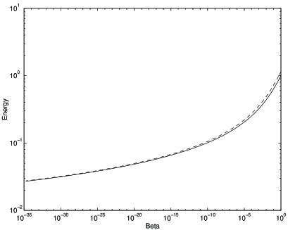
Figure 1: $\mu$ as a function of $\beta$

The energy per unit length of the static vortex solution for the $\phi^{4}$ potential (full line) and the $\phi^{8}$ potential (dashed line). The energy per unit length is in units of $\pi M^{2}$.

5.3 Global symmetry defects

Although a GUT is initially constructed to satisfy a gauge symmetry, global symmetries could occur accidentally and be spontaneously broken by fields with vevs at the same scale $\sim 10^{16}\,\mbox{GeV}$. Global symmetries, notably the Peccei-Quinn $U(1)$ symmetry have also been proposed at lower energies. In addition to the possibilities of monopoles and strings, there are now the possibilities of domain walls and textures. We discuss textures first.

5.3.1 Textures

It is known that textures with a vev $M\sim 10^{16}\,\mbox{GeV}$ can significantly affect the cmb anisotropy and large scale structure [57]. Again, the central question we want to answer is whether the flatness of the potential alters this situation. As with strings, the configuration approaches a scaling solution so the only thing we have to worry about is the energy of the textures for a given vev $M$. The scaling solution for textures is characterized by continuous texture formation on the horizon scales and their subsequent collapse, as governed by the scalar field ordering dynamics.

It turns out that the relevant mass scale is not affected by the flatness of the potential. We will now argue that this is indeed so. The size of the self-coupling $\lambda$ does not matter as long as it is large enough to confine $\Phi$ to the vacuum given by $|\Phi|=M$. Since we are interested in the epoch relevant for structure formation, the relevant scale is $T_{dec}\sim 1eV$, which is much below any scale in the microscopic theory. Indeed the ‘flatness scale’ is given by the curvature of the potential at its minimum $m=V^{\prime\prime}(M)^{1/2}\sim m_{0}\sim 1\,\mbox{TeV}>>T_{dec}$. A more rigorous argument can be constructed by looking at the evolution equation for textures in an expanding Universe. This equation has an effective self-coupling re-scaled as $\lambda_{eff}\sim(a(T)/a_{0})^{2}\lambda$ [58], where $a$ is the scale factor of the Universe. At $T\sim T_{dec}$, the ratio $a(T_{dec})/a_{0}\simeq T_{GUT}/T_{dec}$ is so big that $\lambda_{eff}\sim(m_{0}/T_{dec})^{2}>>1$ is still very large. This means that the effective coupling for all practical purposes is large and the field is confined to $|\Phi|=M$. This implies that the non-linear $\sigma$-model [58] is a very accurate description of the texture dynamics, even for flat potentials. Normalising to the $10^{o}$ scales reported by COBE, and using the cosmological parameters $\Omega=1,\,\Lambda=0$ and $h=0.5$ the result may be read off from [53]: $M\simeq 1.4\times 10^{16}$GeV.

A possible realization of a texture model within grand unified theories is proposed in [59] in which the GUT of the form $G\times SU(3)_{fam}$ (where $SU(3)_{fam}$ is an additional global family symmetry) has been considered. A supersymmetric GUT group with a flat Higgs potential may have a similar form. The family symmetry $SU(3)_{fam}$ breaks with the GUT, so it is plausible to assume that the texture potential is also flat.

5.3.2 Global monopoles and domain walls

The dynamics of global field ordering with SO(3) symmetry (global monopoles) can be studied using similar numerical techniques as developed for textures [53]. Also the ordering dynamics can be to a good approximation represented by a non-linear $\sigma$-model [61], [53]. They eventually reach a scaling solution in which ‘monopoles’ form on the scales of the horizon and then collapse to the core size given by $\sim 1/m_{0}$. Since the interactions between monopoles are strong and long range, there will be a strong tendency for monopole-anti-monopole annihilation which will keep the number of monopoles (anti-monopoles) at the level of order one per horizon at any time. In that respect, the monopole dynamics resembles the dynamics of textures, with an important difference of an occasional monopole – anti-monopole annihilation event, which will tend to imprint a strong non-Gaussian signal on the cmbr. Recalling the assumptions made in their calculation concerning the values of the cosmological parameters we have read off from [53] that global monopoles have an observable signature on large scale structure and/or the cmb anisotropy for some vev of order $M\simeq 1\times 10^{16}$GeV.

For walls we can make a simple estimate based on the energy per unit area of the wall: $\sigma\simeq\int dz[(d\phi/dz)^{2}/2+V(z)]$. Making the simple substitutions $d/dz\sim 1/l$, $\int dz\sim l$, $V(z)\sim V_{0}\sim(m_{0}M)^{2}$, we have $\sigma\sim M^{2}/l+V_{0}l$, which is extremized when $l\sim M/\sqrt{V_{0}}\sim 1/m_{0}$ so that the energy per unit area is about $\sigma\sim M^{3}(m_{0}/M)$, where $m_{0}\sim 10^{3}\,\mbox{GeV}$. Compared with the usual case one sees that walls are much fatter, but less massive. However, the reduction in mass is far too small to allow them to be cosmologically viable. Instead they had better either not form or disappear harmlessly, which is quite possible since the discrete symmetry leading to their appearance will probably be slightly broken if it is not a gauge symmetry [15].

6 Conclusion

The topics discussed in this paper relate to a considerable body of ongoing research at the moment, whose common theme is the form of the effective potential in the early universe, and the consequent cosmological effects of the scalar fields. Some of this research continues to address the traditional, and still very important, question of how to implement an early era of ordinary (slow-roll) inflation. Here we have focussed instead on aspects of ‘thermal inflation’, which occurs if at all after ordinary inflation and lasts for only a few $e$-folds.

The fields which can give rise to thermal inflation are ‘flaton’ fields. By definition, these fields have ‘flat’ potentials and ‘large’ vevs, where these terms refer to the mass scale $10^{2}$ to $10^{3}\,\mbox{GeV}$. They arise naturally in currently favoured extensions of the Standard Model, along with the opposite case of fields with ‘flat’ potentials but zero vevs.

A flaton field gives rise to thermal inflation if it is trapped at the origin by virtue of the finite temperature correction to its effective potential, after the thermal contribution to the energy density has become comparatively small. According to a calculation made a decade ago by Yamamoto, this trapping is expected to occur for a flat potential (provided that the flaton field is indeed in the vicinity of the origin), with thermal inflation ending only when the local minimum of the effective potential at the origin almost completely disappears. Part of our objective was to investigate carefully the rather delicate assumptions needed to arrive at this conclusion, using some modern perspectives particularly on the tunneling rate out of the false vacuum. Happily, we confirm the conclusion.

The actual cosmology of flaton fields, which determines whether a given flaton field will actually find itself in the vicinity of the origin so that thermal inflation can take place, is at present a rather rapidly moving research area. We have not attempted any new advance here, contenting ourselves with a brief snapshot of the situation as it stands at present. Instead we have addressed a question which has received relatively little attention, which is the nature and cosmology of topological defects forming at the end of thermal inflation. One would expect a priori that their cosmology might be significantly affected by the flatness of the potential. The answer to this question turns out to depend on the type of defect.

A particular focus for the second part of our investigation has been the possibility that there is a GUT, whose Higgs fields have a flat potential. This possibility is quite natural, and it leads to a cosmology very different from the usually considered case of a non-flat Higgs potential. GUT symmetry breaking, if it occurs, will be preceded by an era of thermal inflation. The Higgs particles produced at the transition are cosmologically dangerous because they are light and long-lived, and to dilute them one needs a second era of thermal inflation. This period of thermal inflation will also dilute the monopole abundance sufficiently, but will not eliminate cosmic strings because it lasts only a few $e$-folds. A simple picture of a string network evolution in an inflationary Universe is as follows. First as the Universe expands the strings will quickly reach the density of about one (long) string per horizon volume. After that the network freezes out since there exists no causal process that could incite nontrivial dynamics. This means that from then on the average correlation length grows exponentially as the expansion rate, i.e. as $\xi(t)=\xi(t_{0})\,{\rm e}^{H(t-t_{0})}$. After about 10 $e$-foldings the correlation length has not grown more than $\xi\sim{\rm e}^{10}/H$; this scale will come back within the horizon after $\ln(a/a_{0})\sim 10$ which in radiation era means at the temperature $T=T_{D}\times{\rm e}^{-10}\simeq T_{D}\times 10^{-4.3}$; after this strings will quickly reach the radiation era scaling solution. This temperature is far above the relevant scale for onset of cmbr anisotropies and structure formation, keeping the strings cosmologically interesting.

With all this in mind, we expect that cosmological relevance of cosmic strings is specified solely by the mass per unit length of strings. We find that the GUT Higgs vev needed for the strings to give an observable signature in the cmb anisotropy is a few times bigger than in the case of a non-flat potential, but still compatible with the typical estimate $\simeq 2\times 10^{16}\,\mbox{GeV}$ of the scale at which the Standard Model gauge couplings become unified. Perhaps the main message is that the flatness of the potential has surprisingly little effect on the string cosmology.

We also discuss global defects, and in particular focus on the case of global textures and monopoles. We arrive to a rather surprising conclusion that global texture and monopole dynamics is not affected at all by the flatness of the potential. This has a simple explanation: the potential is simply not flat enough! The ‘flatness scale’ $m_{0}\sim 10^{3}$GeV is large in comparison to the scale relevant for cosmology: $T\sim 1$eV, so the flat potential suffices to confine late textures to the vacuum manifold. This leaves both textures and global monopoles as a viable candidate for structure formation with the scales of symmetry breaking given by $M\sim 1.4\times 10^{16}$GeV and $M\sim 1\times 10^{16}$GeV, respectively. Finally in passing we give an argument that domain walls are still a problem.

In summary, the study of fields with flat potentials and large vevs is becoming another field on which particle physics increasingly meets cosmology. Our hope is that either cosmology will put constraints on particle physics models, or particle physics will offer some interesting cosmological phenomena, at best tell us something about the origin of structures in the Universe. Since this area of research is developing very fast, it is very likely that in near future one will be able to make more definite statements about the formation and nature of defects in theories with flat potentials, and hence make a more definite prediction on their cosmological relevance.

Acknowledgements

We thank David Bailin, Beatriz de Carlos, Anne Davis, Andrei Linde, Graham Ross and Ewan Stewart for useful discussions. T.P. acknowledges support from PPARC and NSF. T.B. acknowledges support from JNICT (Portugal).

References

- [1]
- [2] M. Grisaru, W. Siegel, and M. Rocek, Nucl. Phys. B 159 429 (1979)
- [3] N. Seiberg, Phys. Lett. B 318 469 (1993)
- [4] K. Yamamoto, Phys. Lett. 161B, 289 (1985).
- [5] G. D. Coughlan et al., Phys. Lett. 131B, 59 (1983).
- [6] M. Dine, W. Fischler and D. Nemeschansky, Phys. Lett. 136B, 169 (1984).
- [7] G. D. Coughlan, R. Holman, P. Ramond and G. G. Ross, Phys. Lett. 140B, 44 (1984).
- [8] K. Yamamoto, Phys. Lett. 168B, 341 (1986).
- [9] G. Lazarides, C. Panagiotakopoulos and Q. Shafi, Phys. Rev. Lett. 56, 557 (1986).
- [10] K. Enqvist, D. V. Nanopoulos and M. Quiros, Phys. Lett. 169B, 343 (1986).
- [11] O. Bertolami and G. G. Ross, Phys. Lett. B183, 163 (1987).
- [12] K. Yamamoto, Phys. Lett. B194, 390 (1987).
- [13] J. Ellis, K. Enqvist, D. V. Nanopoulos and K. A. Olive, Phys. Lett. B188, 415 (1987); G. Lazarides, C. Panagiotakopoulos and Q. Shafi, Nucl. Phys. B307, 937 (1988); J. Ellis, K. Enqvist, D. V. Nanopoulos and K. A. Olive, Phys. Lett. B225, 313 (1989).
- [14] D. H. Lyth and E. D. Stewart, Phys. Rev. Lett. 75, 201 (1995).
- [15] D. H. Lyth and E. D. Stewart, hep-ph/9510204, to appear in Phys. Rev. D.
- [16] L. Kofman, A. D. Linde and A. A. Starobinsky, hep-th/9510119 (1995).
- [17] For reviews of supersymmetry, see H. P. Nilles, Phys. Rep. 110, 1 (1984) and D. Bailin and A. Love, Supersymmetric Gauge Field Theory and String Theory, IOP, Bristol (1994).
- [18] D.-G. Lee and R. N. Mohapatra, hep-ph/9502210; B. Brahmachari and R. N. Mohapatra, hep-ph/9505347; J. Sato, hep-ph/9508269; B. Brahmachari and R. N. Mohapatra, hep-ph/9508293.
- [19] M. Dine et al., Nucl. Phys. B259, 549 (1985); F. del Aguila, G. Blair, M. Daniel and G. G. Ross, Nucl. Phys. B272, 413 (1986); B. R. Greene, K. H. Kirklin, P. J. Miron and G. G. Ross, Nucl. Phys. B292, 606 (1987); G. Dvali and Q. Shafi, Phys. Lett. B339, 241 (1994); G. Aldazabal, A. Font, L. E. Ibáñez and A. M. Uranga, hep-th/9410206; L. J. Hall and S. Raby, Phys. Rev. D51, 6524 (1995); L. E. Ibáñez, hep-th/9505098; G. Aldazabal, A. Font, L. E. Ibáñez and A. M. Uranga, hep-th/9508033.
- [20] H. Murayama, H. Suzuki and T. Yanagida, Phys. Lett. B291, 418 (1992); D. H. Lyth, in preparation.
- [21] J. Ellis, D. V. Nanopoulos and M. Quiros, Phys. Lett. B174, 176 (1986); B. de Carlos, J. A. Casas, F. Quevedo and E. Roulet, Phys. Lett. B318, 447 (1993).
- [22] T. Banks, D. B. Kaplan and A. E. Nelson, Phys. Rev. D49, 779 (1994).
- [23] L. Randall and S. Thomas, Nucl. Phys. B449, 229 (1995).
- [24] T. Banks, M. Berkooz and P. J. Steinhardt, Phys. Rev. D52, 705 (1995).
- [25] M. Dine, L. Randall and S. Thomas, Phys. Rev. Lett. 75, 398 (1995).
- [26] E. D. Stewart, in preparation.
- [27] A. D. Linde, personal communication and hep-th/9601083.
- [28] E. J. Copeland, A. R. Liddle, D. H. Lyth, E. D. Stewart and D. Wands, Phys. Rev. D49, 6410 (1994).
- [29] S. Weinberg, Phys. Rev. D(, 3357 (1974); G. Dvali, A. S. Melfo and G. Senjanovic, hep-ph/9507230.
- [30] J. H. Traschen and R. H. Brandenberger, Phys. Rev. D42, 2491 (1990).
- [31] L. Kofman, A. D. Linde and A. A. Starobinsky, Phys. Rev. Lett. 73, 3195 (1994).
- [32] Y. Shtanov, J. Traschen and R. Brandenberger, Phys. Rev. D51, 5438 (1995).
- [33] D. Boyanovsky and H. J. de Vega, Phys. Rev. D47, 2343 (1993); D. Boyanovsky, D.-S. Lee and A. Singh, Phys. Rev. D48, 800 (1993); D. Boyanovsky, H. J. de Vega and R. Holman, Phys. Rev. D49, 2769 (1994); D. Boyanovsky, M. D’Attanasio, H. J. de Vega, R. Holman, and D.-S. Lee Phys. Rev. D 52, 6805 (1995), hep-ph/9507414; D.Boyanovsky et al., hep-ph/9511361 (1995).
- [34] M. Yoshimura, hep-th/9506176, Prog. Theor. Phys. 94, 873 (1995); D. I. Kaiser, astro-ph/9507108 (1995); H. Fujisaki et al., hep-ph/9508378 (1995); H. Fujisaki et al., hep-ph/9511381 (1995).
- [35] B. A. Ovrut and P. J. Steinhardt, Phys. Lett. 147B, 263 (1984).
- [36] E. D. Stewart, personal communication.
- [37] L. Dolan and R. Jackiw, Phys. Rev. D 9, 3320 (1974)
- [38] S. Coleman, Phys. Rev. D 15, 2929 (1977); C.G. Callan & S. Coleman, Phys. Rev. D 16, 1762 (1977)
- [39] A. Linde, Phys. Lett. 70B, 306 (1977); ibid. 92B, 119 (1980); A. Linde, Nucl. Phys. B 216, 421 (1983); ERRATUM: ibid. B 223, 544 (1983).
- [40] M. E. Carrington, J. I. Kapusta Phys. Rev. D 47, 5304 (1993).
- [41] G. Moore, T. Prokopec, Phys. Rev. D 52, 7182 (1995), hep-ph/9506475.
- [42] J. Ellis et al., Nucl. Phys. B373, 399 (1992).
- [43] R. Jeannerot and A. C. Davis, hep-ph/9501275 (1995); R. Jeannerot, hep-ph/9509365 (1995)
- [44] A. Vilenkin and E. P. S. Shellard, Cosmic Strings and other Topological Defects, Cambridge University Press, Cambridge (1994).
- [45] E. Parker, Astrophys. J. 160, 383 (1970).
- [46] G. Lazarides, Q. Shafi, and T. F. Walsh, Phys. Lett. 100 B, 21 (1981).
- [47] V. A. Rubakov, JETP Lett. 33, 644 (1981); C. G. Callan, Phys. Rev. D 25, 2141 (1981); F. Wilczek, Phys. Rev. Lett. 48, 1146 (1982).
- [48] R. Kolb, S. A. Colgate, and J. Harvey, Phys. Rev. Lett. 49, 1373 (1982); S. Dimopoulos, J. Preskill, and F. Wilczek, Phys. Lett. 119 B, 32 (1982).
- [49] R. Gregory, W. Perkins, A.C. Davis and R.H. Brandenberger, in The Formation and Evolution of Cosmic Strings, eds. G. Gibbons, S.W. Hawking and T. Vachaspati (CUP 1990).
- [50] E.J. Copeland, D. Haws, T.W.B. Kibble, D. Mitchell and N. Turok, Nucl. Phys. B298, 445 (1988).
- [51] M. B. Hindmarsh, Astrophys. J. 431, 534 (1994).
- [52] M. B. Hindmarsh and T. W. B. Kibble, Rep. Prog. Phys. 58, 477 (1995).
- [53] D. Coulson, P. Ferreira, P. Graham and N. Turok, Nature 368, 27 (1994)
- [54] T. Vachaspati and A. Vilenkin, Phys. Rev. Lett. 67, 1057 (1991).
- [55] E.B. Bogomol’nyi, Sov. J. Nucl. Phys. 23, 558 (1976).
- [56] L. Jacobs and C. Rebbi, Phys. Rev. B19, 4486 (1979).
- [57] N. Turok, Phys. Rev. Lett. 63 2625 (1989).
- [58] N. Turok and D. Spergel, Phys. Rev. Lett. 64 2736 (1990); D. N. Spergel, N. Turok, W. H. Press, B. S. Ryden Phys. Rev. D 43 1038 (1991).
- [59] M. Joyce and N. Turok, Nucl. Phys. B416, 389 (1994), hep-ph/9301287.
- [60] R. A. Battye and E. P. S. Shellard, Phys. Rev. Lett. 73, 2954 (1994).
- [61] D. P. Bennett and S. H. Rhie, Astrophys. J. 406 L7 (1993).