Perturbative corrections to zero recoil inclusive $B$ decay sum rules

Abstract

Comparing the result of inserting a complete set of physical states in a time ordered product of $b$ decay currents with the operator product expansion gives a class of zero recoil sum rules. They sum over physical states with excitation energies less than $\Delta$, where $\Delta$ is much greater than the QCD scale and much less than the heavy charm and bottom quark masses. These sum rules have been used to derive an upper bound on the zero recoil limit of the $B\to D^{*}$ form-factor, and on the matrix element of the kinetic energy operator between $B$ meson states. Perturbative corrections to the sum rules of order $\alpha_{s}(\Delta)\,\Delta^{2}/m_{c,b}^{2}$ have previously been computed. We calculate the corrections of order $\alpha_{s}(\Delta)$ and $\alpha_{s}^{2}(\Delta)\,\beta_{0}$ keeping all orders in $\Delta/m_{c,b}$, and show that these perturbative QCD corrections suppressed by powers of $\Delta/m_{c,b}$ significantly weaken the upper bound on the zero recoil $B\to D^{*}$ form-factor, and also on the kinetic energy operator’s matrix element.

Over the last six years, dramatic progress has been achieved in our understanding of exclusive and inclusive $B$ decays. For exclusive decays this resulted from applying heavy quark symmetry [1] to relate $B$ decay form-factors and obtain their normalization at zero recoil. For example, the form-factors that occur in $B\to D\,e\,\bar{\nu}_{e}$ and $B\to D^{*}\,e\,\bar{\nu}_{e}$ semileptonic decays are related by heavy quark symmetry to a single universal function of $v\cdot v^{\prime}$ ($v$ is the four-velocity of the $B$, and $v^{\prime}$ is that of the recoiling $D^{(*)}$), and furthermore, this function is normalized to unity at zero recoil [1, 2, 3, 4].

Progress in the theory of inclusive $B$ decays has come from applying the operator product expansion and heavy quark effective theory [5] to perform a $1/m_{b}$ expansion of the time ordered product of $b$ decay currents [6]. It was found that at leading order in this expansion, the inclusive semileptonic $B$ decay rate is equal to the perturbative $b$ quark decay rate. There are no nonperturbative corrections at order $1/m_{b}$, and the corrections of order $1/m_{b}^{2}$ are characterized by only two matrix elements (we use the standard relativistic normalization for the $B$ meson states)

$$\lambda_{1}={1\over 2m_{B}}\,\langle B(v)\,|\,\bar{h}_{v}^{(b)}\,(iD)^{2}\,h_{v}^{(b)}\,|\,B(v)\rangle\,,$$ (1)

and

$$\lambda_{2}={1\over 6m_{B}}\,\langle B(v)\,|\,\bar{h}_{v}^{(b)}\,{g\over 2}\,\sigma_{\mu\nu}\,G^{\mu\nu}\,h_{v}^{(b)}\,|\,B(v)\rangle\,,$$ (2)

where $h_{v}^{(b)}$ is the $b$ quark field in the heavy quark effective theory [7, 8, 9]. The matrix element $\lambda_{2}$ is scale dependent [10], and it is determined from the measured $B^{*}-B$ mass splitting, $\lambda_{2}(m_{b})\simeq 0.12\,{\rm GeV}^{2}$.

Sum rules have been derived that relate exclusive decay form-factors to the matrix elements $\lambda_{1,2}$ [11]. The zero recoil sum rules follow from analysis of the time ordered product

$$T_{\mu\nu}={i\over 2m_{B}}\,\int{\rm d}^{4}x\,e^{-iq\cdot x}\,\langle B\,|\,T\{J_{\mu}^{\dagger}(x),J_{\nu}(0)\}|B\,\rangle\,,$$ (3)

where $J_{\nu}$ is a $b\to c$ axial or vector current, the $B$ states are at rest, $\vec{q}=0$ and $q^{0}=m_{b}-m_{c}-\epsilon$. Viewed as a function of complex $\epsilon$, $T_{\mu\nu}$ has two cuts along the real $\epsilon$-axis. One, for $\epsilon\gtrsim 0$, corresponds to physical states with a charm quark and the other, for $\epsilon\lesssim-2m_{c}$, corresponds to physical intermediate states with two $b$ quarks and a $\bar{c}$ quark. The first cut arises from inserting the states between the two currents in the product $J^{\dagger}J$, and the second cut arises from inserting the states between the currents in the other time ordering $JJ^{\dagger}$. So we arrive at

$$T_{\mu\nu}(\epsilon) = {1\over 2m_{B}}\,\sum_{X}\,(2\pi)^{3}\,\delta^{3}(\vec{p}_{X})\,{\langle B|J_{\mu}^{\dagger}|X\rangle\langle X|J_{\nu}|B\rangle\over(m_{b}-m_{c})-(m_{B}-m_{X})-\epsilon-i\,0}$$ (4)

$$- {1\over 2m_{B}}\,\sum_{X}\,(2\pi)^{3}\,\delta^{3}(\vec{p}_{X})\,{\langle B|J_{\nu}|X\rangle\langle X|J_{\mu}^{\dagger}|B\rangle\over(m_{b}-m_{c})+(m_{B}-m_{X})-\epsilon+i\,0}\,.$$ (5)

The sum over $X$ includes the usual phase space factors, i.e., ${\rm d}^{3}p/2E$ for each particle in the state $X$.

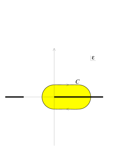
FIG. 1.: The integration contour $C$ in the complex $\epsilon$ plane. The cuts extend to ${\rm Re}\,\epsilon\to\pm\infty$.

Consider integration of the product of a weight function $W_{\Delta}(\epsilon)$ with $T_{\mu\nu}(\epsilon)$ along the contour $C$ shown in Fig. 1. Assuming $W$ is analytic in the shaded region enclosed by this contour and averaging over $\mu=\nu=1,2,3$, we get

$${1\over 2\pi i}\,\int_{C}\,{\rm d}\epsilon\,W_{\Delta}(\epsilon)\,{T_{ii}(\epsilon)\over 3}=\sum_{X}\,W_{\Delta}[(m_{X}-m_{c})-(m_{B}-m_{b})]\,(2\pi)^{3}\,\delta^{3}(\vec{p}_{X})\,{\Big{|}\langle X|J_{i}|B\rangle\Big{|}^{2}\over 3\cdot 2m_{B}}\,.$$ (6)

The maximum $X$ mass on the right-hand side of eq. (6) is determined by where the contour $C$ pinches the real axis. For convenience this mass is chosen to be less than $2m_{b}+m_{c}$ to prevent the occurrence of states $X$ with $b$, $\bar{b}$, and $c$ quarks. We take the maximum $X$ mass to be $2m_{B}$. Hereafter it is understood that sums over $X$ only go over states up to mass $2m_{B}$.

We require that: ($i$) the weight function $W_{\Delta}$ be positive semidefinite along the cut so that every term in the sum over $X$ on the right-hand side of eq. (6) is non-negative; ($ii$) $W_{\Delta}(0)=1$; ($iii$) $W_{\Delta}$ be flat near $\epsilon=0$ (i.e., at least ${\rm d}W_{\Delta}(\epsilon)/{\rm d}\epsilon\Big{|}_{\epsilon=0}=0$); ($iv$) and that it falls off rapidly to zero for $\epsilon>\Delta$. We want to take $\Delta\ll m_{c,b}$. Then states $X$ other than the $D^{*}$ give a contribution to the right-hand side of eq. (6) that is suppressed by $(1/m_{c,b})^{2}$. However, in our numerical results we consider $\Delta$ as large as $2\,$GeV. Although our analysis holds for any weight function that satisfies these four properties, for explicit calculations we use

$$W_{\Delta}^{(n)}(\epsilon)={\Delta^{2n}\over\epsilon^{2n}+\Delta^{2n}}\,,$$ (7)

with $n=2,3,\ldots$ (for $n=1$ the integral over $\epsilon$ is dominated by contributions from states with mass of order $m_{B}$). These weight functions have poles at $\epsilon=\root 2n \of{-1}\,\Delta$, therefore, as long as $n$ is not too large and $\Delta$ is much larger than the QCD scale, $\Lambda_{\rm QCD}$, the contour in Fig. 1 is far from the cut until $\epsilon$ is near $2m_{B}$. Then we should be able to calculate the integral in eq. (6) using the operator product expansion to evaluate the time ordered product.

The choice of the set of weight functions in eq. (7) is motivated by the fact that for values of $n$ of order unity all poles of $W_{\Delta}^{(n)}$ lie at a distance of order $\Delta$ away from the physical cut. In this case the integral along the contour $C$ can be computed only assuming local duality [12] at the scale $2m_{B}$. The dependence of our results on this assumption is extremely weak, because for $\Delta\ll m_{B}$ the weight function is very small where the contour $C$ touches the cut. As $n\to\infty$, $W_{\Delta}^{(n)}$ approaches $\theta(\Delta-\epsilon)$ for positive $\epsilon$, which corresponds to summing over all hadronic resonances up to excitation energy $\Delta$ with equal weight. Then the poles of $W_{\Delta}^{(n)}$ approach the cut, and the contour $C$ is forced to lie within distance of order $\Delta/n$ from the cut at $\epsilon=\Delta$. In this case the evaluation of the integral along the contour $C$ relies also on local duality at the scale $\Delta$.

Neglecting perturbative QCD corrections and nonperturbative effects corresponding to operators of dimension greater than five, the operator product expansion gives [9]

$$\frac{1}{3}\,T_{ii}^{AA}=-\frac{1}{\epsilon}+{(\lambda_{1}+3\lambda_{2})(m_{b}-3m_{c})\over 6m_{b}^{2}\,\epsilon\,(2m_{c}+\epsilon)}-{4\lambda_{2}m_{b}-(\lambda_{1}+3\lambda_{2})(m_{b}-m_{c}-\epsilon)\over m_{b}\,\epsilon^{2}\,(2m_{c}+\epsilon)}\,,$$ (8)

when $J_{\mu}=A_{\mu}=\bar{c}\,\gamma_{\mu}\gamma_{5}\,b$, and

$$\frac{1}{3}\,T_{ii}^{VV}=-\frac{1}{2m_{c}+\epsilon}+{(\lambda_{1}+3\lambda_{2})(m_{b}+3m_{c})\over 6m_{b}^{2}\,\epsilon\,(2m_{c}+\epsilon)}-{4\lambda_{2}m_{b}-(\lambda_{1}+3\lambda_{2})(m_{b}-m_{c}-\epsilon)\over m_{b}\,\epsilon\,(2m_{c}+\epsilon)^{2}}\,,$$ (9)

when $J_{\mu}=V_{\mu}=\bar{c}\,\gamma_{\mu}\,b$. Performing the contour integration yields

$$\frac{1}{6m_{B}}\, \sum_{X}\,W_{\Delta}[(m_{X}-m_{c})-(m_{B}-m_{b})]\,(2\pi)^{3}\,\delta^{3}(\vec{p}_{X})\,\Big{|}\langle X|A_{i}|B\rangle\Big{|}^{2}$$ (12)

$$=1-{\lambda_{2}\over m_{c}^{2}}+\bigg{(}{\lambda_{1}+3\lambda_{2}\over 4}\bigg{)}\bigg{(}\frac{1}{m_{c}^{2}}+\frac{1}{m_{b}^{2}}+\frac{2}{3m_{c}m_{b}}\bigg{)}\,,$$

$$\frac{1}{6m_{B}}\, \sum_{X}\,W_{\Delta}[(m_{X}-m_{c})-(m_{B}-m_{b})]\,(2\pi)^{3}\,\delta^{3}(\vec{p}_{X})\,\Big{|}\langle X|V_{i}|B\rangle\Big{|}^{2}$$ (14)

$$={\lambda_{2}\over m_{c}^{2}}-\bigg{(}{\lambda_{1}+3\lambda_{2}\over 4}\bigg{)}\bigg{(}\frac{1}{m_{c}^{2}}+\frac{1}{m_{b}^{2}}-\frac{2}{3m_{c}m_{b}}\bigg{)}\,.$$

These equations hold for any $W_{\Delta}$ that satisfies the four properties mentioned above. Higher order terms in the operator product expansion for $T_{ii}$ give contributions with more factors of $1/\epsilon$ on the right-hand sides of eqs. (8) and (9). Therefore, if the weight function has nonvanishing $m$’th derivative at $\epsilon=0$, there are corrections to the right-hand side of eq. (12) of order

$$\bigg{(}{\Lambda_{\rm QCD}\over m_{c,b}}\bigg{)}\bigg{(}{\Lambda_{\rm QCD}\over\Delta}\bigg{)}^{\!m}=\bigg{(}{\Lambda_{\rm QCD}\over m_{c,b}}\bigg{)}^{\!2}\,\bigg{[}\bigg{(}{m_{c,b}\over\Lambda_{\rm QCD}}\bigg{)}\bigg{(}{\Lambda_{\rm QCD}\over\Delta}\bigg{)}^{\!m}\bigg{]}\,.$$ (15)

We require that $\Delta$ be large enough compared with the QCD scale $\Lambda_{\rm QCD}$, so that such terms are smaller than those we kept in eq. (12). For $m>1$ $\Delta$ can still be smaller than $m_{c,b}$. Higher order terms in the operator product expansion of $T_{ii}^{VV}$ give corrections to the right-hand side of eq. (14) of order $(\Lambda_{\rm QCD}/m_{c,b})^{2}\,(\Lambda_{\rm QCD}/\Delta)^{m-1}$. This is why we imposed condition ($iii$). For the weight function $W^{(n)}_{\Delta}(\epsilon)$ in eq. (7) the first nonvanishing derivative is at $m=2n$.

We have considered the nonperturbative corrections to the sum rules (9) characterized by $\lambda_{1}$ and $\lambda_{2}$. There are also perturbative corrections suppressed by powers of the strong coupling. These are most easily calculated not in the operator product expansion, but by directly considering the sum over states in (9) and replacing the hadronic states by quark and gluon states. The perturbative corrections are of two types. There are corrections of order $\alpha_{s}(m_{c,b})$ not suppressed by powers of $\Delta/m_{c,b}$. These arise, at the parton level, from the final state $X=c$ and change the term $1$ on the right-hand side of (12) to $\eta_{A}^{2}$, where $\eta_{A}$ is the usual factor that relates the axial current in the full theory of QCD to the axial current in the heavy quark effective theory (at zero recoil). $\eta_{A}$ has been calculated to order $\alpha_{s}$ [3], and terms of order $\alpha_{s}^{2}\,\beta_{0}$, where $\beta_{0}=(11-\frac{2}{3}\,n_{f})$, are also known [13, 14]. Explicitly,

$$\eta_{A}=1-{\alpha_{s}\over\pi}\,\bigg{(}{m_{b}+m_{c}\over m_{b}-m_{c}}\ln{m_{c}\over m_{b}}+\frac{8}{3}\bigg{)}-{\alpha_{s}^{2}\over\pi^{2}}\,\beta_{0}\,\frac{5}{24}\,\bigg{(}{m_{b}+m_{c}\over m_{b}-m_{c}}\ln{m_{c}\over m_{b}}+\frac{44}{15}\bigg{)}\,,$$ (16)

where $\alpha_{s}$ is the $\overline{\rm MS}$ coupling evaluated at the scale $\sqrt{m_{b}m_{c}}$.

There is another class of perturbative QCD corrections coming from final states $X$ that contain a charm quark plus additional partons, e.g., $c\,g$, $c\,\bar{q}\,q$, etc. They give a contribution to the right-hand side of equations (9) that is of order $[\alpha_{s}(\Delta)+\ldots]\,F(\Delta)$, where the ellipses denote terms of higher order in the strong coupling constant $\alpha_{s}$, and for small $\Delta$, $F(\Delta)\sim\Delta^{2}/m_{c,b}^{2}$. We have evaluated the strong coupling constant at the scale $\Delta$, because that characterizes the typical hadronic mass in the sum over $X$. Note that although these corrections are suppressed by powers of $\Delta/m_{c,b}$ they can be as important as the other perturbative corrections we considered, since the strong coupling constant is evaluated at a lower scale $\Delta$. The value for these corrections depends on the precise form of the weight function, and we use the ones given in eq. (7). Such perturbative corrections were calculated at order $\alpha_{s}(\Delta)\,\Delta^{2}/m_{c,b}^{2}$ in the limit when the weight function approaches the step-function $\theta(\Delta-\epsilon)$ (corresponding to $W_{\Delta}^{(\infty)}$) [11, 15]. As we have already pointed out, the use of such a weight function relies on local duality at the scale $\Delta$, so the corrections are expected to be less than those stemming from $W_{\Delta}^{(n)}$ with small $n$ relying on local duality only at the scale $2m_{B}$. We calculated for $n\geq 2$ the terms of order $\alpha_{s}(\Delta)$ coming from the Feynman diagrams in Fig. 2, and the order $\alpha_{s}^{2}(\Delta)\,\beta_{0}$ terms arising from the diagrams shown in Fig. 3. Then eqs. (12) and (14) become

FIG. 2.: Feynman diagrams that contribute to the order $\alpha_{s}(\Delta)$ corrections to the sum rules. The black square indicates insertion of the $b\to c$ axial or vector current.

FIG. 3.: Feynman diagrams that determine the order $\alpha_{s}^{2}(\Delta)\,\beta_{0}$ corrections to the sum rules.

$$\frac{1}{6m_{B}}\, \sum_{X}W_{\Delta}^{(n)}[(m_{X}-m_{c})-(m_{B}-m_{b})]\,(2\pi)^{3}\,\delta^{3}(\vec{p}_{X})\,\Big{|}\langle X|A_{i}|B\rangle\Big{|}^{2}$$ (18)

$$= \eta_{A}^{2}-{\lambda_{2}\over m_{c}^{2}}+\bigg{(}{\lambda_{1}+3\lambda_{2}\over 4}\bigg{)}\bigg{(}\frac{1}{m_{c}^{2}}+\frac{1}{m_{b}^{2}}+\frac{2}{3m_{c}m_{b}}\bigg{)}+{\alpha_{s}(\Delta)\over\pi}\,X_{AA}^{(n)}(\Delta)+{\alpha_{s}^{2}(\Delta)\over\pi^{2}}\,\beta_{0}\,Y_{AA}^{(n)}(\Delta)\,,$$ (19)

$$\frac{1}{6m_{B}}\, \sum_{X}W_{\Delta}^{(n)}[(m_{X}-m_{c})-(m_{B}-m_{b})]\,(2\pi)^{3}\,\delta^{3}(\vec{p}_{X})\,\Big{|}\langle X|V_{i}|B\rangle\Big{|}^{2}$$ (20)

$$= {\lambda_{2}\over m_{c}^{2}}-\bigg{(}{\lambda_{1}+3\lambda_{2}\over 4}\bigg{)}\bigg{(}\frac{1}{m_{c}^{2}}+\frac{1}{m_{b}^{2}}-\frac{2}{3m_{c}m_{b}}\bigg{)}+{\alpha_{s}(\Delta)\over\pi}\,X_{VV}^{(n)}(\Delta)+{\alpha_{s}^{2}(\Delta)\over\pi^{2}}\,\beta_{0}\,Y_{VV}^{(n)}(\Delta)\,.$$ (21)

On the right-hand sides of eqs. (3) terms suppressed by more than two powers of $\Lambda_{\rm QCD}/m_{c,b}$ or $\alpha_{s}$ have been neglected. We have also neglected in (18) terms suppressed by $(\Lambda_{\rm QCD}/m_{c,b})\,(\Lambda_{\rm QCD}/\Delta)^{2n}$ and in (20) terms suppressed by $(\Lambda_{\rm QCD}/m_{c,b})^{2}\,(\Lambda_{\rm QCD}/\Delta)^{2n-1}$. Perturbative corrections to the terms proportional to $\lambda_{1,2}$ are also neglected, and we evaluate $\lambda_{2}$ in eqs. (3) at the scale $m_{b}$ (a calculation of QCD corrections to its coefficient would resolve this scale ambiguity). For $\Delta\ll m_{c,b}$ the functions $X^{(n)}$ and $Y^{(n)}$ are given by

$$X_{AA}^{(n)}(\Delta) = \Delta^{2}\,{A^{(n)}\over 3}\,\bigg{(}\frac{1}{m_{c}^{2}}+\frac{1}{m_{b}^{2}}+\frac{2}{3m_{c}m_{b}}\bigg{)}\,,$$ (22)

$$X_{VV}^{(n)}(\Delta) = \Delta^{2}\,{A^{(n)}\over 3}\,\bigg{(}\frac{1}{m_{c}^{2}}+\frac{1}{m_{b}^{2}}-\frac{2}{3m_{c}m_{b}}\bigg{)}\,,$$ (23)

$$Y_{AA}^{(n)}(\Delta) = \Delta^{2}\,{B^{(n)}\over 6}\,\bigg{(}\frac{1}{m_{c}^{2}}+\frac{1}{m_{b}^{2}}+\frac{2}{3m_{c}m_{b}}\bigg{)}+\Delta^{2}\,{A^{(n)}\over 15}\,\bigg{(}\frac{1}{m_{c}^{2}}+\frac{1}{m_{b}^{2}}+\frac{4}{3m_{c}m_{b}}\bigg{)}\,,$$ (24)

$$Y_{VV}^{(n)}(\Delta) = \Delta^{2}\,{B^{(n)}\over 6}\,\bigg{(}\frac{1}{m_{c}^{2}}+\frac{1}{m_{b}^{2}}-\frac{2}{3m_{c}m_{b}}\bigg{)}\,,$$ (25)

where the coefficients $A^{(n)}$ and $B^{(n)}$ are ($n\geq 2$)

$$A^{(n)}={\pi\over n\sin(\pi/n)}\,,\qquad B^{(n)}=A^{(n)}\,\bigg{(}{\pi\over 2n\tan(\pi/n)}+\frac{5}{3}-\ln 2\bigg{)}\,.$$ (26)

For $\Delta$ near $1\,$GeV higher powers of $\Delta/m_{c,b}$ are important. The analytic expressions for $X^{(\infty)}_{AA}$ and $X^{(\infty)}_{VV}$ are (for $\Delta<2m_{b}$)

$$X_{AA}^{(\infty)} = {\Delta\,(\Delta+2m_{c})\,[2(\Delta+m_{c})^{2}-2m_{b}^{2}-(m_{b}+m_{c})^{2}]\over 18m_{b}^{2}\,(\Delta+m_{c})^{2}}+{3m_{b}^{2}+2m_{b}m_{c}-m_{c}^{2}\over 9m_{b}^{2}}\,\ln{\Delta+m_{c}\over m_{c}}\,,$$ (27)

$$X_{VV}^{(\infty)} = {\Delta\,(\Delta+2m_{c})\,[2(\Delta+m_{c})^{2}-2m_{b}^{2}-(m_{b}-m_{c})^{2}]\over 18m_{b}^{2}\,(\Delta+m_{c})^{2}}+{3m_{b}^{2}-2m_{b}m_{c}-m_{c}^{2}\over 9m_{b}^{2}}\,\ln{\Delta+m_{c}\over m_{c}}\,.$$ (28)

($X_{AA}^{(\infty)}$ was also calculated in Ref. [15]. Our result seems to disagree with theirs.) In Figures 4a and 4b we plot $X^{(\infty)}$ and $Y^{(\infty)}$ versus $\Delta$ using the values $m_{b}=4.8\,$GeV and $m_{c}=1.4\,$GeV. The thick solid lines are $X$ and the thick dashed lines are $Y$, while the thin lines are the corresponding functions at order $\Delta^{2}/m_{c,b}^{2}$. Note that expanding in $\Delta/m_{c,b}$ is not a good approximation unless $\Delta\lesssim 400\,$MeV.

FIG. 4.: $X^{(\infty)}(\Delta)$ and $Y^{(\infty)}(\Delta)$ for the a) axial, and b) vector coefficients. Thick solid lines are $X$ while thick dashed lines are $Y$. The thin solid and dashed lines are $X$ and $Y$ to order $\Delta^{2}/m_{c,b}^{2}$.

The evaluation of the order $\alpha_{s}^{2}\,\beta_{0}$ corrections is made relatively simple by the relation between the $n_{f}$ dependent part of the order $\alpha_{s}^{2}$ contribution and the order $\alpha_{s}$ contribution with a finite gluon mass [16]. Such a relation holds in the so-called $V$-scheme, but throughout this paper we present all results in the usual $\overline{\rm MS}$ scheme. Knowledge of the order $\alpha_{s}^{2}\,\beta_{0}$ corrections allows us to obtain the BLM scale [17] that results from absorbing vacuum polarization effects into the running coupling constant. It is generally believed that this choice of scale yields a reasonable perturbative expansion. This is also the reason for using $\alpha_{s}(\Delta)$ in the sum rules in eqs. (3). Had we chosen some very different scale $\mu$, the coefficients $Y^{(n)}$ would contain large logarithms of $\mu^{2}/\Delta^{2}$. Using $m_{b}=4.8\,$GeV, $m_{c}=1.4\,$GeV, and $n\to\infty$ we obtain $\mu_{\rm BLM}^{AA}\simeq 0.12\Delta$ and $\mu_{\rm BLM}^{VV}\simeq 0.17\Delta$ for the BLM scales for the axial and vector current sum rules, respectively. If we demand $\alpha_{s}(\mu_{\rm BLM})<1$, then $\Delta$ needs to be above about $3-4\,$GeV, which would completely eliminate the restrictive power of the sum rules. Another possibility, which we adopt, is just to use our results as estimates of the $\alpha_{s}^{2}$ corrections, but to retain $\Delta\simeq 1\,$GeV. Then we find that the order $\alpha_{s}^{2}(\Delta)$ corrections to the sum rules are comparable to the order $\alpha_{s}(\Delta)$ terms, and we can only hope that terms of higher order in $\alpha_{s}(\Delta)$ are not similarly important.

The parameters $\lambda_{1}$ and $\lambda_{2}$ also occur in the inclusive differential $B$ decay rate, which can be expressed in terms of the $B$ and $D$ meson masses and the parameters $\lambda_{1}$, $\lambda_{2}$ and $\bar{\Lambda}$, where

$$m_{B}=m_{b}+\bar{\Lambda}-{\lambda_{1}+3\lambda_{2}\over 2m_{b}}\,,\qquad m_{D}=m_{c}+\bar{\Lambda}-{\lambda_{1}+3\lambda_{2}\over 2m_{c}}\,.$$ (30)

The pole mass is not a physical quantity, and the perturbative expression for the $\overline{\rm MS}$ mass $\overline{m_{b}}(m_{b})$ in terms of the pole mass $m_{b}$ is not Borel summable, giving rise to what is sometimes called a “renormalon ambiguity” in the pole mass [18]. However, when the differential semileptonic decay rate is expressed in terms of the hadron masses and $\bar{\Lambda}$, the perturbative QCD corrections to the decay rate are also not Borel summable. If $\bar{\Lambda}$ (or equivalently the $b$ quark pole mass) extracted from the differential semileptonic decay rate is used to get the $\overline{\rm MS}$ mass these ambiguities cancel, so one can arrive at a meaningful prediction for the $\overline{\rm MS}$ $b$ quark mass. It is fine to introduce unphysical quantities like $\bar{\Lambda}$ as long as one works consistently to a given order of QCD perturbation theory and the expansion in inverse powers of the heavy quark masses. Since the final results one considers always involve relations between physically measurable quantities, any “renormalon ambiguities” arising from the bad behavior of the QCD perturbation series at large orders will cancel out [19, 20]. As the left-hand sides of the sum rules in eqs. (3) are physical quantities, the right-hand sides, when calculated to all orders in $\alpha_{s}$, should be free of renormalon ambiguities. We checked that the order $\Lambda_{\rm QCD}^{2}/m_{c,b}^{2}$ renormalon ambiguity in the quantity $\eta_{A}^{2}$ [20] cancels against that in the perturbative corrections suppressed by $\Delta^{2}/m_{c,b}^{2}$ (such a cancellation was conjectured in [21]).

Eqs. (12) and (14) have been used to bound the $B\to D^{*}$ zero recoil form-factor [22, 11]. The sum rule (18) implies a bound on the zero recoil $B\to D^{*}$ matrix element of the axial current $F_{B\to D^{*}}^{2}$, defined by $\langle D^{*}|A_{i}|B\rangle=2\sqrt{m_{D^{*}}m_{B}}\,F_{B\to D^{*}}\,\varepsilon_{i}$, that reads

$$F_{B\to D^{*}}^{2} \leq \eta_{A}^{2}-{\lambda_{2}\over m_{c}^{2}}+\bigg{(}{\lambda_{1}+3\lambda_{2}\over 4}\bigg{)}\bigg{(}\frac{1}{m_{c}^{2}}+\frac{1}{m_{b}^{2}}+\frac{2}{3m_{c}m_{b}}\bigg{)}$$ (31)

$$+ {\alpha_{s}(\Delta)\over\pi}\,X_{AA}^{(n)}(\Delta)+{\alpha_{s}^{2}(\Delta)\over\pi^{2}}\,\beta_{0}\,Y_{AA}^{(n)}(\Delta)\,.$$ (32)

Here we used that the contributions of states $X$ of higher mass than the $D^{*}$ to the left-hand side of (18) are positive, and neglected the very small deviation of $W_{\Delta}^{(n)}[(m_{D^{*}}-m_{c})-(m_{B}-m_{b})]$ from unity implied by eq. (7), eq. (30), and the relation $m_{D^{*}}-m_{D}=2\lambda_{2}/m_{c}$. The positivity of the sum over states $X$ in eq. (20) implies that

$$0\leq{\lambda_{2}\over m_{c}^{2}}-\bigg{(}{\lambda_{1}+3\lambda_{2}\over 4}\bigg{)}\bigg{(}\frac{1}{m_{c}^{2}}+\frac{1}{m_{b}^{2}}-\frac{2}{3m_{c}m_{b}}\bigg{)}+{\alpha_{s}(\Delta)\over\pi}\,X_{VV}^{(n)}(\Delta)+{\alpha_{s}^{2}(\Delta)\over\pi^{2}}\,\beta_{0}\,Y_{VV}^{(n)}(\Delta)\,.$$ (33)

This inequality gives a constraint on the heavy quark effective theory matrix element $\lambda_{1}$, which is strongest when one takes the $m_{c}\gg m_{b}\gg\Delta$ limit, giving

$$\lambda_{1}\leq-3\lambda_{2}+{\alpha_{s}(\Delta)\over\pi}\,\Delta^{2}\,{4A^{(n)}\over 3}+{\alpha_{s}^{2}(\Delta)\over\pi^{2}}\,\beta_{0}\,\Delta^{2}\,{2B^{(n)}\over 3}\,.$$ (34)

		$n=2$	$n=3$	$n=\infty$
$\lambda_{1}$	to order $\alpha_{s}$	$-0.06\,GeV^{2}$	$-0.13\,GeV^{2}$	$-0.17\,GeV^{2}$
	to order $\alpha_{s}^{2}\,\beta_{0}$	$0.13\,GeV^{2}$	$0.06\,GeV^{2}$	$0.01\,GeV^{2}$
$F_{B\to D^{*}}$	to order $\alpha_{s}$	$0.96$	$0.96$	$0.95$
	to order $\alpha_{s}^{2}\,\beta_{0}$	$0.99$	$0.99$	$0.98$

TABLE I.: Upper limits on $\lambda_{1}$ and $F_{B\to D^{*}}$ that can be obtained from the sum rules in eqs. (31) and (34) with $\Delta=1\,$GeV. $n$ labels the weight function $W_{\Delta}^{(n)}$.

Neglecting the perturbative corrections suppressed by powers of $\alpha_{s}(\Delta)$, eq. (34) yields $\lambda_{1}\leq-0.36\,{\rm GeV}^{2}$, which in turn implies using eq. (31) that $F_{B\to D^{*}}\leq 0.93$ [22]. (With $m_{b}=4.8\,$GeV and $m_{c}=1.4\,$GeV we find $\eta_{A}=0.96$ following from eq. (16).) To indicate the importance of the perturbative corrections proportional to $\alpha_{s}(\Delta)$ and $\alpha_{s}^{2}(\Delta)\,\beta_{0}$, we give the bounds that result when they are included for $n=2$, $n=3$, and $n\to\infty$ in Table I. The effects of these corrections are smaller if we choose $\Delta$ small (corresponding to suppressing the contribution of higher excited states) or if we choose $n$ large (using local duality at the scale $\Delta$). Note that while it is plausible that $n$ can be chosen arbitrarily large as local duality is expected to hold at scales much above $\Lambda_{\rm QCD}$, the relation $\Delta\gg\Lambda_{\rm QCD}$ must be maintained and so $\Delta$ cannot be chosen to be less than about $1\,$GeV. Using $n_{f}=3$, $\Delta=1\,$GeV and $\alpha_{s}(1\,{\rm GeV})=0.45$ we obtain the bounds given in Table I. The large magnitude of the second order corrections to the sum rules indicates that the series of perturbative corrections might be under control only for $\Delta$ significantly above $1\,$GeV. Such a value for $\Delta$ would greatly weaken the restrictive power of the sum rules. Similar comments and conclusions apply to two analogous sum rules derived for $B^{*}\to D^{(*)}$ transitions in Ref. [23].

In conclusion, we investigated perturbative corrections to the zero recoil inclusive $B$ decay sum rules derived in Ref. [11]. We calculated the corrections suppressed by powers of $\Delta/m_{c,b}$ at order $\alpha_{s}(\Delta)$ and order $\alpha_{s}^{2}(\Delta)\,\beta_{0}$ corresponding to a set of possible weight functions that determine the contributions of excited hadronic intermediate states. These corrections significantly weaken the constraints stemming from the sum rules. It is widely believed that $\lambda_{1}<0$ (although in our opinion it has not been proven in QCD for $\lambda_{1}$ defined by the $\overline{\rm MS}$ subtraction scheme), and we are not aware of any claim that $F_{B\to D^{*}}$ is significantly above 1. Due to the size of the $\Delta$-dependent terms in the sum rules, it is hard to deduce any useful model independent bounds. An upper bound below 1 on the zero recoil $B\to D^{*}$ form-factor barely survives these perturbative corrections, and a limit on $\lambda_{1}$ that restricts it to negative values does not. However, it is important to remember that the results in Table I rely on the applicability of QCD perturbation theory at a scale $\Delta=1\,$GeV, and furthermore are very sensitive to the value of $\alpha_{s}$ at this scale. In the future $\lambda_{1}$ may be determined from experimental data on inclusive $B$ decays [24], and then a bound on $F_{B\to D^{*}}$ that does not rely on eq. (34) can be derived from eq. (31).

In light of our discussion, we see no reason to think that the original estimates of $F_{B\to D^{*}}$, based on model calculations, the structure of terms arising at order $1/m_{c,b}^{2}$ [25], and on chiral perturbation theory [26], badly underestimated the $1/m_{c,b}^{2}$ corrections. Our results show that the zero recoil sum rules do not demand a larger deviation of $F_{B\to D^{*}}$ from $\eta_{A}$, even if the $D^{*}$ does not saturate the sum over states $X$. We cannot prove at this point that such a deviation does not occur. However, in the absence of any such indication, it is most natural to think that $F_{B\to D^{*}}\simeq\eta_{A}=0.96$ holds to an accuracy of about the canonical size of the $1/m_{c,b}^{2}$ corrections, that is within $(500\,{\rm MeV}/2m_{c})^{2}\simeq 3\%$.

REFERENCES

[1]
N. Isgur and M.B. Wise, Phys. Lett. B232 (1989) 113;
Phys. Lett. B237 (1990) 527.
[2]
S. Nussinov and W. Wetzel, Phys. Rev. D36 (1987) 130.
[3]
M. Voloshin and M. Shifman, Sov. J. Nucl. Phys. 47 (1988) 511.
[4]
M.E. Luke, Phys. Lett. B252 (1990) 447.
[5]
E. Eichten and B. Hill, Phys. Lett. B234 (1990) 511;
H. Georgi, Phys. Lett. B240 (1990) 447.
[6]
J. Chay, H. Georgi and B. Grinstein, Phys. Lett. B247 (1990) 399;
M. Voloshin and M. Shifman, Sov. J. Nucl. Phys. 41 (1985) 120.
[7]
I.I. Bigi, N.G. Uraltsev and A.I. Vainshtein, Phys. Lett. B293 (1992) 430
[(E) ibid. B297 (1993) 477];
I.I. Bigi, M. Shifman, N.G. Uraltsev, and A. Vainshtein,
Phys. Rev. Lett. 71 (1993) 496.
[8]
A.V. Manohar and M.B. Wise, Phys. Rev. D49 (1994) 1310;
T. Mannel, Nucl. Phys. B413 (1994) 396.
[9]
B. Blok, L. Koyrakh, M. Shifman and A.I. Vainshtein,
Phys. Rev. D49 (1994) 3356 [(E) ibid. D50 (1994) 3572].
[10]
G.P. Lepage and B.A. Thacker, Nucl. Phys. B (Proc. Suppl.) 4 (1988) 199;
E. Eichten and B. Hill, Phys. Lett. B243 (1990) 427;
A.F. Falk, B. Grinstein and M.E. Luke, Nucl. Phys. B357 (1991) 185.
[11]
I.I. Bigi, M.A. Shifman, N.G. Uraltsev, and A.I. Vainshtein,
Phys. Rev. D52 (1995) 196.
[12]
E.C. Poggio, H.R. Quinn, and S. Weinberg, Phys. Rev. D13 (1976) 1958.
[13]
M. Neubert, Phys. Lett. B341 (1995) 367.
[14]
Corrections of order have also been calculated for
various inclusive semileptonic decay distributions:
M. Luke, M.J. Savage, and M.B. Wise, Phys. Lett. B343 (1995) 329;
Phys. Lett. B345 (1995) 301;
A.F. Falk, M. Luke, and M.J. Savage, hep-ph/9507284.
[15]
J.G. Korner, K. Melnikov, and O. Yakovlev, hep-ph/9502377.
[16]
B.H. Smith and M.B. Voloshin, Phys. Lett. B340 (1994) 176.
[18]
I.I. Bigi, M.A. Shifman, N.G. Uraltsev and A.I. Vainshtein,
Phys. Rev. D50 (1994) 2234;
M. Beneke and V.M. Braun, Nucl. Phys. B426 (1994) 301.
[19]
M. Beneke, V.M. Braun, and V.I. Zakharov, Phys. Rev. Lett. 73 (1994) 3058;
M. Luke, A.V. Manohar, and M.J. Savage, Phys. Rev. D51 (1995) 4924.
[20]
M. Neubert and C.T. Sachrajda, Nucl. Phys. B438 (1995) 235.
[21]
M. Shifman, hep-ph/9409358.
[22]
M.A. Shifman, N.G. Uraltsev, and A.I. Vainshtein,
Phys. Rev. D51 (1995) 2217 [(E) ibid. D52 (1995) 3149].
[23]
M. Neubert, Phys. Lett. B338 (1994) 84.
[24]
Z. Ligeti and Y. Nir, Phys. Rev. D49 (1994) 4331;
A. Kapustin and Z. Ligeti, Phys. Lett. B355 (1995) 318;
A.F. Falk, M. Luke, and M. Savage, hep-ph/9511454.
[25]
A.F. Falk and M. Neubert, Phys. Rev. D47 (1993) 2965;
T. Mannel, Phys. Rev. D50 (1994) 428.
[26]
L. Randall and M.B. Wise, Phys. Lett. B303 (1993) 135.