Triple Gauge Boson Couplings

Conveners: G. Gounaris, J.-L. Kneur and D. Zeppenfeld

Working group: Z. Ajaltouni, A. Arhrib, G. Bella, F. Berends, M. Bilenky, A. Blondel,
J. Busenitz, D. Charlton, D Choudhury, P. Clarke, J. E. Conboy, M. Diehl, D. Fassouliotis,
J.-M. Frère, C. Georgiopoulos, M. Gibbs, M. Grünewald, J. B. Hansen, C. Hartmann,
B. N. Jin, J. Jousset, J. Kalinowski, M. Kocian, A. Lahanas, J. Layssac, E. Lieb, C. Markou,
C. Matteuzzi, P. Mättig, J. M. Moreno, G. Moultaka, A. Nippe, J. Orloff, C. G. Papadopoulos,
J. Paschalis, C. Petridou, H. Phillips, F. Podlyski, M. Pohl, F. M. Renard, J.-M. Rossignol,
R. Rylko, R. L. Sekulin, A. van Sighem, E. Simopoulou, A. Skillman, V. Spanos, A. Tonazzo,
M. Tytgat, S. Tzamarias, C. Verzegnassi, N. D. Vlachos, E. Zevgolatakos

1. Introduction

2. Parametrization, models and present bounds on TGC

3. The W pair production process

4. Statistical techniques for TGC determination

5. Precision of TGC determination at LEP2: generator level studies

6. Analysis of the $jje\nu$ and $jj\mu\nu$ final states

7. Analysis of the $jj\tau\nu$ final state

8. Analysis of the $jjjj$ final state

9. Analysis of the $\ell\nu\ell\nu$ final state

10. Other anomalous couplings and other channels

11. Conclusions

1 Introduction

Present measurements of the vector boson-fermion couplings at LEP and SLC accurately confirm the Standard Model (SM) predictions at the 0.1 – 1% level [1], which may readily be considered to be evidence for the gauge boson nature of the W and the Z. Nevertheless the most crucial consequence of the $SU(2)\times U(1)$ gauge theory, namely the specific form of the non-Abelian self-couplings of the W, Z and photon, remains poorly measured to date. A direct and more accurate measurement of the trilinear self-couplings is possible via pair production of electroweak bosons in present and future collider experiments ($W^{+}W^{-}$ at LEP2, $W\gamma$, $WZ$ and $W^{+}W^{-}$ at hadron colliders).

The major goal of such experiments at LEP2 will be to corroborate the SM predictions. If sufficient accuracy is reached, such measurements can be used to probe New Physics (NP) in the bosonic sector. This possibility raises a number of other questions. What are the expected sizes of such effects in definite models of NP? What type of specifically bosonic NP contributions could have escaped detection in other experiments, e.g. at LEP1? Are there significant constraints from low-energy measurements? Although we shall address these questions, the aim of this report is mostly to elaborate on a detailed phenomenological strategy for the direct measurement of the self-couplings at LEP2, which should allow their determination from data with the greatest possible accuracy.

2 Parametrization, Models and Present Bounds on TGC

We shall restrict ourselves to Triple Gauge boson Couplings (TGC) in most of the report (possibilities to test quartic couplings at LEP2 are extremely limited). Analogous to the introduction of arbitrary vector and axial-vector couplings $g_{V}$ and $g_{A}$ of the gauge bosons to fermions, the measurements of the TGC can be made quantitative by introducing a more general WWV vertex. We thus start with a parametrization in terms of a purely phenomenological effective Lagrangian  [2, 3] [$V\equiv\gamma$ or $Z$]

$$i{\cal L}_{eff}^{WWV} = g_{WWV}\,\Bigl{[}g_{1}^{V}V^{\mu}\left(W^{-}_{\mu\nu}W^{+\nu}-W^{+}_{\mu\nu}W^{-\nu}\right)+\kappa_{V}\,W^{+}_{\mu}W^{-}_{\nu}V^{\mu\nu}+$$

$${\lambda_{V}\over m_{W}^{2}}\,V^{\mu\nu}W^{+\rho}_{\!\!\nu}W^{-}_{\rho\mu}+ig_{5}^{V}\varepsilon_{\mu\nu\rho\sigma}\left((\partial^{\rho}W^{-\mu})W^{+\nu}-W^{-\mu}(\partial^{\rho}W^{+\nu})\right)V^{\sigma}$$

$$+ig_{4}^{V}W^{-}_{\mu}W^{+}_{\nu}(\partial^{\mu}V^{\nu}+\partial^{\nu}V^{\mu})-\frac{\tilde{\kappa}_{V}}{2}W^{-}_{\mu}W^{+}_{\nu}\varepsilon^{\mu\nu\rho\sigma}V_{\rho\sigma}-{\tilde{\lambda}_{V}\over{2m_{W}^{2}}}\,W^{-}_{\rho\mu}{W^{+\mu}}_{\nu}\varepsilon^{\nu\rho\alpha\beta}V_{\alpha\beta}\Bigr{]}\;,$$

which gives the most general Lorentz invariant $WWV$ vertex observable in processes where the vector bosons couple to effectively massless fermions. Here the overall couplings are defined as $g_{WW\gamma}=e$ and $g_{WWZ}=e\cot\theta_{W}$, $W_{\mu\nu}=\partial_{\mu}W_{\nu}-\partial_{\nu}W_{\mu}$, and $V_{\mu\nu}=\partial_{\mu}V_{\nu}-\partial_{\nu}V_{\mu}$. For on-shell photons, $g_{1}^{\gamma}(q^{2}=0)=1$ and $g_{5}^{\gamma}(q^{2}=0)=0$ are fixed by electromagnetic gauge invariance Within the SM, at tree level, the couplings are given by $g_{1}^{Z}=g_{1}^{\gamma}=\kappa_{Z}=\kappa_{\gamma}=1$, with all other couplings in (2) vanishing. Terms with higher derivatives in (2) are equivalent to a dependence of the couplings on the vector boson momenta and thus merely lead to a form-factor behaviour of them. We also note that $g_{1}^{V}$, $\kappa_{V}$ and $\lambda_{V}$ conserve $C$ and $P$ separately, while $g_{5}^{V}$ violates $C$ and $P$ but conserves $CP$. Finally $g_{4}^{V}$, $\tilde{\kappa}_{V}$ and $\tilde{\lambda}_{V}$ parameterize a possible CP violation in the bosonic sector, which will not be much studied in this report, as it may be considered a more remote possibility for LEP2 studies . However, there exist definite and simple means to test for such CP violation, see section 3. The $C$ and $P$ conserving terms in ${\cal L}_{eff}^{WW\gamma}$ correspond to the lowest order terms in a multipole expansion of the $W-$photon interactions: the charge $Q_{W}$, the magnetic dipole moment $\mu_{W}$ and the electric quadrupole moment $q_{W}$ of the $W^{+}$ [5]:

$$Q_{W}~{}=~{}eg_{1}^{\gamma}\;~{}~{},~{}~{}\mu_{W}~{}=~{}{e\over 2m_{W}}\left(g_{1}^{\gamma}+\kappa_{\gamma}+\lambda_{\gamma}\right)\;,~{}~{}q_{W}~{}=~{}-{e\over m_{W}^{2}}\left(\kappa_{\gamma}-\lambda_{\gamma}\right)\;.$$ (2)

For practical purposes it is convenient to introduce deviations from the (tree-level) SM as

$$\Delta g_{1}^{Z}\equiv(g_{1}^{Z}-1)~{}~{}\equiv\tan\theta_{W}\delta_{Z}~{},~{}~{}~{}\Delta\kappa_{\gamma}\equiv(\kappa_{\gamma}-1)~{}~{}\equiv\mbox{$x_{\gamma}$}~{},$$ (3)

$$\Delta\kappa_{Z}\equiv(\kappa_{Z}-1)~{}~{}\equiv\tan\theta_{W}(x_{Z}+\delta_{Z})~{},$$

$$\lambda_{\gamma}~{}~{}\equiv y_{\gamma},~{}~{}~{}\lambda_{Z}~{}~{}\equiv\tan\theta_{W}\,y_{Z}\;.$$

For completeness (and easy comparison) the correspondence of the most studied C and P conserving parameters has also been given for another equivalent set ($\delta_{Z},\;x_{V},\;y_{V}$), which was used in some recent analyses [6, 7].

2.1 Gauge-invariant Parametrization of TGC

Any of the interaction terms in (2) can be rendered $SU(2)\times U(1)$ gauge invariant by adding to it interactions involving additional gauge bosons [8], and/or additional Would Be Goldstone Bosons (WBGBs) and the physical Higgs (if it exists)[9, 10, 11]. However, one needs to consider $SU(2)\times U(1)$ gauge invariant operators of high dimension in order to reproduce all couplings in (2). For example, if the Higgs particle exists one needs to consider operators of dimension up to $d=12$. Depending on the NP dynamics, such operators could be generated at the NP mass scale $\Lambda_{NP}$, with a strength which is generally suppressed by factors like $(m_{W}/\Lambda_{NP})^{d-4}$ or $(\sqrt{s}/\Lambda_{NP})^{d-4}$ [12, 13]. Accordingly, the gauge invariance requirement alone does not provide any constraint on the form of possible interactions. Rather it is a low energy approximation, the neglect of operators of dimension greater than 4 or 6, which leads to relations among the various TGCs.

Such relations among TGCs are highly desirable, given the somewhat limited statistics accessible at LEP2. They were first derived in  [14, 8] by imposing approximate global $SU(2)$ symmetry conditions on the phenomenological Lagrangian (2). In the next subsection we present them following an approach based on $SU(2)\times U(1)$ gauge invariance and dimensional considerations. The connection to the approach based on “global $SU(2)$” symmetry will be discussed at the end.

In order to write down all allowed operators of a given dimensionality one must first identify the low energy degrees of freedom participating in NP. We assume that these include only the $SU(2)\times U(1)$ gauge fields and the remnants of the spontaneous breaking of the gauge symmetry, the WBGBs that exist already in the standard model. If a relatively light Higgs boson is assumed to exist, then NP is described in terms of a direct extension of the ordinary SM formalism; i.e. using a linear realization of the symmetry. On the other hand, if the Higgs is absent from the spectrum (or, equivalently for our purpose, if it is sufficiently heavy), then the effective Lagrangian should be expressed using a nonlinear realization of the symmetry.

2.1.1 Linear Realization

In addition to a Higgs doublet field $\Phi$, the building blocks of the gauge-invariant operators are the covariant derivatives of the Higgs field, $D_{\mu}\Phi$, and the non-Abelian field strength tensors $\hat{W}_{\mu\nu}=W_{\mu\nu}-gW_{\mu}\times W_{\nu}$ and $B_{\mu\nu}$ of the $SU(2)_{L}$ and $U(1)_{Y}$ gauge fields respectively.

Considering CP-conserving interactions of dimension $d=6$, 11 independent operators can be constructed [15, 9, 10]. Four of these operators affect the gauge boson propagators at tree level [16] and as a result their coefficients are severely constrained by present low energy data [9, 10]. Another subset of these operators generates anomalous Higgs couplings and will be discussed in section 10.4 below. Here we consider the three remaining operators which do not affect the gauge boson propagators at tree-level, but give rise to deviations in the C and P-conserving TGC. Denoting the corresponding couplings as $\alpha_{W\phi}$, $\alpha_{B\phi}$, and $\alpha_{W}$, the TGC inducing effective Lagrangian is written as

$${\cal L}^{TGC}_{d=6}=ig^{\prime}{\mbox{$\alpha_{B\phi}$}\over m^{2}_{W}}\,(D_{\mu}\Phi)^{\dagger}B^{\mu\nu}(D_{\nu}\Phi)\,+\,ig{\mbox{$\alpha_{W\phi}$}\over m^{2}_{W}}\,(D_{\mu}\Phi)^{\dagger}\vec{\tau}\cdot\vec{\hat{W}}^{\mu\nu}(D_{\nu}\Phi)\,+g{\mbox{$\alpha_{W}$}\over{6m^{2}_{W}}}\,\vec{\hat{W}}^{\mu}_{\phantom{\mu}\nu}\cdot(\vec{\hat{W}}^{\nu}_{\phantom{\nu}\rho}\times\vec{\hat{W}}^{\rho}_{\phantom{\rho}\mu})\,,$$ (4)

with $g$, $g^{\prime}$ the $SU(2)_{L}$ and $U(1)_{Y}$ couplings respectively. Replacing the Higgs doublet field by its vacuum expectation value, $\Phi^{T}\to(0,v/\sqrt{2})$, yields nonvanishing anomalous TGCs in (2),

$$\Delta g_{1}^{Z}=\frac{\mbox{$\alpha_{W\phi}$}}{c^{2}_{W}}\;,\qquad\Delta\kappa_{\gamma}=-\frac{c^{2}_{W}}{s^{2}_{W}}(\Delta\kappa_{Z}-\Delta g_{1}^{Z})=\mbox{$\alpha_{W\phi}$}+\mbox{$\alpha_{B\phi}$}\;,\qquad\lambda_{\gamma}=\lambda_{Z}=\mbox{$\alpha_{W}$}\;,$$ (5)

where $s_{W}\equiv\sin\theta_{W}$, $c_{W}\equiv\cos\theta_{W}$. The normalization of the dimension 6 operators in (4) has been chosen such that the coefficients $\alpha_{i}$ correspond directly to $\Delta\kappa_{\gamma}$ and $\lambda_{\gamma}$. It should be noted that, as the NP scale $\Lambda_{NP}$ is increased, the $\alpha_{i}$ are expected to decrease as $(m_{W}/\Lambda_{NP})^{2}$.

This scaling behaviour can be quantified to some extent by invoking (tree-level) unitarity constraints [17, 18, 19, 13]. A constant anomalous TGC leads to a rapid growth of vector boson pair production cross-sections with energy, saturating the unitarity limit at $\sqrt{s}=\Lambda_{U}$. A larger value of $\Lambda_{U}$ implies a smaller TGC $\alpha_{i}$. For each of them the unitarity relation may be written as [17, 18]

$$|\mbox{$\alpha_{W}$}|\simeq 19~{}\left({m_{W}\over\Lambda_{U}}\right)^{2},\ \ |\mbox{$\alpha_{W\phi}$}|\simeq 15.5\left({m_{W}\over\Lambda_{U}}\right)^{2},\ \ |\mbox{$\alpha_{B\phi}$}|\simeq 49\left({m_{W}\over\Lambda_{U}}\right)^{2}.$$ (6)

For any given value of $\alpha_{i}$ the corresponding scale $\Lambda_{U}$ provides an upper bound on the NP scale $\Lambda_{NP}$. Conversely, a sensitivity to small values of an anomalous coupling constant is equivalent to a sensitivity to potentially high values of the corresponding NP scale. Applying (6) for $\Lambda_{U}=1$ TeV, we get $|\mbox{$\alpha_{W}$}|\simeq 0.12$, $|\mbox{$\alpha_{W\phi}$}|\simeq 0.1$, $|\mbox{$\alpha_{B\phi}$}|\simeq 0.3$. Since these values are larger than the expected LEP2 sensitivity by less than a factor 3, it is clear that LEP2 is sensitive to $\Lambda_{NP}\mathrel{\raise 1.29167pt\hbox{$<$\kern-7.5pt\lower 4.30554pt\hbox{$\sim$}}}1$ TeV. Thus a caveat is in order: for these low values of $\Lambda_{NP}$ the neglect of dimension 8 operators may no longer be justified, leading to deviations from the relations (5)[20].

2.1.2 Nonlinear Realization

In the absence of a light Higgs a non-linear approach should be used to render ${\cal L}^{WWV}_{eff}$ gauge invariant. The SM Lagrangian, deprived of the Higgs field, violates unitarity at a scale of roughly $4\pi v\sim 3$ TeV, so that the new physics should appear at a scale $\Lambda_{NP}\mathrel{\raise 1.29167pt\hbox{$<$\kern-7.5pt\lower 4.30554pt\hbox{$\sim$}}}4\pi v$. Technically the construction of gauge-invariant operators follows closely the linear case above, except that in place of the scalar doublet $\Phi$ a (unitary, dimensionless) matrix $U\equiv\exp(i{\vec{\omega}}\cdot{\vec{\tau}}/v)$, where the $\omega_{i}$ are the WBGBs, and the appropriate matrix form of the $SU(2)_{L}\times U(1)_{Y}$ covariant derivative are used. The so-called “naive dimensional analysis” (NDA) [22] dictates that the expected order of magnitude of a specific operator involving $b$ WBGB fields, $d$ derivatives and $w$ gauge fields is $\sim v^{2}\Lambda_{NP}^{2}\;(1/v)^{b}\;(1/\Lambda_{NP})^{d}\;(g/\Lambda_{NP})^{w}$. Applying NDA to the terms in Eqs. (2), we see that $\Delta g_{1}^{V}$ and $\Delta\kappa_{V}$ are of ${\cal O}(m_{W}^{2}/\Lambda_{NP}^{2})$. In other words, just as in the linear realization, these terms are effectively of dimension 6 (in the sense that there is an explicit factor of $1/\Lambda_{NP}^{2}$). On the other hand, we see that the $W^{\dagger}_{\rho\mu}{W^{\mu}}_{\nu}V^{\nu\rho}$ term is effectively of dimension 8, i.e. the coefficient $\lambda_{V}$ is expected to be of order $m_{W}^{4}/\Lambda_{NP}^{4}$. Thus, within the nonlinear realization scenario, the $\lambda_{V}$ terms are expected to be negligible compared to those proportional to $\Delta g_{1}^{V}$ and $\Delta\kappa_{V}$. Accordingly there remain three parameters at lowest dimensionality, which can be taken as $g_{1}^{Z}$, $\kappa_{Z}$ and $\kappa_{\gamma}$.

2.1.3 Operators of Higher Dimension and Global Symmetry Arguments

As mentioned in section 2.1, one may argue that relations like in (5) would not even be approximately correct if $\Lambda_{NP}$ is substantially smaller than 1 TeV, since higher dimensional operators are no longer suppressed, and may even be more important than the $dim=6$ operators [20]. In fact, as far as the 5 C and P conserving TGC in (2) are concerned, the most general choice can be realized by invoking two $dim=8$ operators in addition to the 3 terms in (4) [10, 11, 23]. Requiring restoration of an $SU(2)$ global (”custodial”) symmetry for $g^{\prime}\to 0$ (i.e in the limit of decoupling B field) implies [23] the coefficient of one of these two operators to vanish, because it violates $SU(2)$ global independently of the B field. In that way one recovers the constraints between $\Delta\kappa_{\gamma}$ and $\Delta\kappa_{Z}$ in (5), in both the nonlinear realization and in the linear realization at the $dim=8$ level. Nevertheless a second $dim=8$ operator spoils the relation, $\lambda_{\gamma}=\lambda_{Z}$ in (5). One may neglect this term (which vanishes in the limit $g^{\prime}\to 0$) by imposing exact $SU(2)$ at the scale $\Lambda_{NP}$, which in our context is similar to neglecting the $\pi^{\pm}-\pi^{0}$ mass difference in strong interaction physics.

Largely these are simplifying assumptions only, intended to reduce the number of free parameters. Motivated by the previous discussion we recommend two sets of three parameters each for full correlation studies between anomalous couplings at LEP2:

• set1 = ($\Delta g_{1}^{Z},\;\Delta\kappa_{\gamma},\;\Delta\kappa_{Z}$) with $\lambda_{\gamma}=\lambda_{Z}=0$. These correspond to the operators of lowest dimensionality in the nonlinear realization. A reduction to 2 parameters (using $\Delta\kappa_{\gamma}=-\frac{c^{2}_{W}}{s^{2}_{W}}(\Delta\kappa_{Z}-\Delta g_{1}^{Z})$) is achieved by assuming [6, 23] custodial $SU(2)$ for $g^{\prime}\to 0$.

• set2 = ($\Delta g_{1}^{Z},\;\Delta\kappa_{\gamma},\;\lambda_{\gamma}$) with $\lambda_{Z}$ and $\Delta\kappa_{Z}$ given by (5). It is this set which has been used in this report for the determination of precisions achievable from $WW$ production at LEP2, presented in sections 5–9 as limits on the parameters $\alpha_{B\phi}$, $\alpha_{W\phi}$ and $\alpha_{W}$ defined by (4).

Expressing results in terms of $\Delta g^{Z}_{1}$, $\Delta\kappa_{\gamma}$, etc. will be useful for ease of comparison with published hadron collider data [25, 26].

In addition, it would clearly be of interest to present fits to each of the parameters in ${\cal L}_{eff}^{WWV}$ in order to reduce the dependence of the analysis on specific models. However, this can only be achieved bearing in mind the limited data which will be available from LEP2, and the correlations inherent in the extraction of many parameters from the data. We return to this point in sections 3.1, 4.2 and 5.1 below.

2.2 Present constraints on TGC

The errors of present direct measurements, via pair production of electroweak bosons at the Tevatron, are still fairly large. The latest, best published 95% CL bounds by $CDF$ and $D0$ are obtained from studies of $W\gamma$ events [25, 26]

$$-1.6<\Delta\kappa_{\gamma}<1.8\;,\qquad-0.6<\lambda_{\gamma}<0.6$$

but constraints from the study of $WW,\;WZ\to\ell\nu jj,\;\ell\ell jj$ events are becoming competitive and should lead to 95% CL bounds of roughly $-0.65<\Delta\kappa_{\gamma}<0.75,\;|\lambda_{\gamma}|=|\lambda_{Z}|<0.4$, once the already collected run 1b data are fully analyzed. Increasing the integrated luminosity to 1 fb${}^{-1}$ with the Fermilab main injector is expected to improve these limits by another factor 2 [27]. Note that these latter bounds assume the relations between anomalous couplings as given by (5) with $\alpha_{W\phi}$ =$\alpha_{B\phi}$. In addition, the Tevatron measures these parameters at considerably larger momentum transfers than LEP2 and, hence, form factor effects could result in different measured values at the two machines.

Alternatively, constraints may be derived also from evaluating virtual contributions of TGC to precisely measured quantities such as $(g-2)_{\mu}$ [28], the $b\to s\gamma$ decay rate [29, 30], $B\to K^{(*)}\mu^{+}\mu^{-}$ [31], the $Z\to b\bar{b}$ [32] rate and oblique corrections[9, 10] (i.e. corrections to the W, Z, $\gamma$ propagators). Oblique corrections combine information from the recent LEP/SLD data, neutrino scattering experiments, atomic parity violation, $\mu$-decay, and the $W$-mass measurement at hadron colliders.

When trying to derive TGC bounds from their virtual contributions one must make assumptions about other NP contributions to the observable in question. In the linear realization, for example, Higgs contributions to the oblique parameters tend to cancel the TGC contributions and as a result the TGC bounds are relatively weak for a light Higgs boson [10]. In general, there are other higher dimensional operators which contribute directly to the observable, in addition to the virtual TGC effects. Bounds on the TGC then require to either specify the underlying model of NP completely or to assume that no significant cancellation occurs. The bounds on the TGC parameters in (2) due to virtual effets thus depend on the underlying hypotheses and are of ${\cal O}(0.1)$ to ${\cal O}(1)$ [9, 10, 33].

More stringent bounds are obtained [9] by comparing the higher dimensional operators which induce TGC with those operators which directly induce oblique effects (see Section 10.1). In simple models the coefficients of these two sets of operators are of similar size and hence the stringent LEP1 bounds on the latter [34] indicate that one should not expect anomalous TGC above ${\cal O}(0.01)$. One should stress, however, that no rigourous relation between oblique effects and TGC can be derived except by going to specific models of NP. Therefore, these stringent bounds must be verified, by a direct measurement of the TGC at LEP2.

2.3 Virtual Contributions to TGC in the MSSM

Definite TGC contributions are certainly present at the loop level in any renormalizable model, although such loop effects contribute to TGC with a factor of $(g^{2}/16\pi^{2})\simeq$ 2.7 10${}^{-3}$, being therefore too small a priori to be observed at LEP2. For instance, SM one-loop TGC predictions are known [35, 36, 37] and give, at $\sqrt{s}=$ 190 GeV, $\Delta\kappa_{\gamma}$ ($\Delta\kappa_{Z}$) $\simeq$ 4.1–5.7 10${}^{-3}$ (3.3–3.1 10${}^{-3}$), for $m_{Higgs}=$ 0.065–1 TeV and $m_{top}=$ 175 GeV [38]. (Contributions to $\lambda_{V}$ are about a factor of 3 smaller). One may, however, expect that the “natural scale” $(g^{2}/16\pi^{2})$ could be substantially enhanced if, for example, some particles in the loop have strong coupling and/or are close to their production threshold. To obtain a “reference point” it is thus important to explore more quantitatively how far one is from the LEP2 accuracy limit, within some well-defined model of NP. We here use the contributions of the (MSSM) [39] as an example. These contributions were calculated independently by two groups in the framework of the Workshop. We summarize the main results, referring for more details to refs. [37, 38].

SUGRA-GUT MSSM	Unconstrained MSSM (maximal effects)
$A_{0},m_{0},M_{1/2}=$ 300,300,80 (GeV),	$\tan\beta=$1.5; $M^{\chi^{+}}_{1,2}\simeq$ 95, 130; $M^{\chi^{0}}_{i}\simeq$ 20–132 (GeV) ;
$\tan\beta=$ 2    ($\mu<0$)	$m_{H+}\simeq$ 95; $m_{\tilde{\nu}_{l}}\simeq$ 45; $m_{\tilde{l}}\simeq$ 92–110; $m_{\tilde{q}}\simeq$45-800 GeV
$|\Delta\kappa_{\gamma}|\!=\!$ 0.44 10${}^{-2}$, $|\Delta\kappa_{Z}|\!=\!$ 0.72 10${}^{-2}$	$\Delta\kappa_{\gamma}=$ 1.75 10${}^{-2}$, $\Delta\kappa_{Z}=$ 0.84 10${}^{-2}$

Table 1: $\Delta\kappa_{\gamma,Z}$ (as defined in eq. 2) in MSSM at $\sqrt{s}=$ 190 GeV. (Contributions to $\lambda_{V}$ are about a factor of 2-3 smaller).

Naively, TGC are obtained by summing all MSSM contributions to the appropriate parts in eq. (2) from vertex loops with entering $\gamma$ (or $Z$) and outgoing $W^{+}$, $W^{-}$. But as is well-known, the vertex graphs with virtual gauge bosons need to be combined with parts of box graphs for the full process, $e^{+}e^{-}\to W^{+}W^{-}$, to form a gauge-invariant contribution. The resulting combinations define purely $s$-dependent TGC [36]. In table 1 we illustrate our results for ($s$-dependent) contributions in two different cases. First, for a representative choice of the free parameters in the more constrained MSSM spectrum obtained [37] from the SUGRA-GUT scenario [40]: the only parameters are the universal soft terms $m_{0}$, $M_{1/2}$, $A_{0}$ at the GUT scale, $\tan\beta$ (and the sign of $\mu$). Second, we give one illustrative contribution, obtained [38] from a rather systematic search of maximal effects in the unconstrained MSSM parameter space. The largest contributions are mostly due to gauginos and/or some of the sleptons and squarks being practically at threshold. One may note, however, that some individual contributions, potentially larger, were quite substantially reduced when the present constraints on the MSSM parameters are taken into account [38]. Even these maximal contributions hardly reach the level of the most optimistic accuracy limit expected on TGC (compare section 5 below). One should also note that radiatively generated TGC generically have a complicated $\sqrt{s}$ form factor dependence as well as contributions from boxes, which are well approximated by an expansion in $1/\Lambda_{NP}$ only when one probes well below threshold.

2.4 TGC from extra $Z^{\prime}$

A light and weakly coupled $Z^{\prime}$ provides an illustrative example of relatively large deviations of the TGC from their SM values and of strong form-factor effects [41]. Consider an extra gauged $U(1)^{\prime}$ symmetry with associated coupling $g^{\prime}_{1}$, whose vector boson $Z^{\prime}$ is relatively light, say $M_{Z^{\prime}}\simeq 200$GeV. For such a boson to remain undetected at LEP1 and CDF, it must have rather small couplings to fermions: $\lambda\equiv\hbox{sin}(\theta_{W})g^{\prime}_{1}/g_{1}<0.2$ or less [41]. However, this new $Z^{\prime}$ might be only part of the new physics beyond the SM, and we parametrize this by gauge invariant higher dimensional operators. For illustration, let us focus on the $dim=6$ operator

$${\cal L}_{B^{\prime}W}\equiv{\epsilon\over v^{2}}O_{B^{\prime}W}={\epsilon\over v^{2}}\phi^{\dagger}B^{\prime\mu\nu}\vec{\hat{W}}_{\mu\nu}\cdot\vec{\tau}\phi$$ (7)

where $B^{\prime}_{\mu\nu}$ is the new $U^{\prime}(1)$ field strength. This operator has a part linear in $W_{\mu}$ inducing unusual mixing through the kinetic terms, from which LEP1 data put upper bounds on $\lambda$ and $\epsilon$. The other piece is quadratic in $W_{\mu}$ and brings anomalous contributions to $W$-pair production at LEP2, which may be enhanced at will by approaching the $Z^{\prime}$ pole. Within a gauge-invariant framework, enlarging the symmetry group has given us enough freedom to escape the more stringent LEP1 constraints on the coefficient of the similar operator ${\cal O}_{BW}$ [9, 10] of Eq. (29). Having such an (admittedly contrived) counter-example to [9] (depending on the 3 parameters $M_{Z^{\prime}}$, $\lambda<0.2$ and $|\epsilon|<0.2$), it is instructive to see how it fits into our TGC parametrization.

# The normal way of extracting the predictions of this model for $W$-pair production would be to add all the amplitudes for $e^{+}e^{-}\rightarrow W^{+}W^{-}$, namely the $t$-channel $\nu$ pole, and $s$-channel $\gamma$, $Z$ and $Z^{\prime}$ poles, including the contributions of $O_{B^{\prime}W}$ in the latter. Alternatively, the correct angular dependence in $\mbox{$e^{+}e^{-}$}\rightarrow\mbox{$W^{+}W^{-}$}$from such a $Z^{\prime}$ is recovered through the introduction of “process – dependent” TGC form factors: the $Z^{\prime}$ exchange only contributes to the $J=1$ partial wave and the TGC of Eq. (2) allow to parameterize the most general $J=1$ amplitude. For the case at hand one can always find TGC $(g^{Z}_{1},\kappa^{Z},g^{\gamma}_{1},\kappa^{\gamma})$ matching the $Z^{\prime}$ parameter dependence in this particular ee-WW channel, but these TGC will depend on the incoming electron’s coupling to the Z and the photon. $\Delta g_{1}^{Z}$ $\Delta g_{1}^{\gamma}$ $\Delta g_{1}^{Z}$ $\Delta g_{1}^{\gamma}$
The deviations $\Delta g_{1}^{Z}$ vs. $\Delta g_{1}^{\gamma}$ for $\sqrt{s}=205$GeV and $M_{Z^{\prime}}=210$GeV. For each $\lambda$ ranging from 0 (plain curve) to 0.2 (smallest dashes), $\epsilon$ is limited to satisfy today’s $W$ mass accuracy, $|\delta M_{W}|<160$MeV (LEP2’s $|\delta M_{W}|<45$MeV for the thick curves). In general, a non-zero $\Delta g^{\gamma}_{1}$ is needed to match the precise $t$-dependence, but in such a process-dependent approach, this does not imply any violation of charge conservation. Finally one should note that the $Z^{\prime}$ described above would also appear in $e^{-}e^{+}\to q\bar{q},\;\ell^{-}\ell^{+}$ at LEP2 and thus all channels need to be searched for NP effects.

3 The $W$ Pair Production Process

3.1 Phenomenology of On-shell $WW$ Production

Deviations of the TGC’s from their SM, tree level form are most directly observed in vector boson pair production. At LEP2 this is the process $e^{-}e^{+}\to W^{-}W^{+}$, which, to lowest order, proceeds via the Feynman graphs of Fig. 1. We start by describing the core process, including the $W$ decay into fermion anti-fermion pairs in the zero-width approximation, since most of the effects of anomalous couplings can already be understood at this level. A full simulation of the signal will, of course, need refinements such as finite width effects, the ensuing contributions from final state radiation graphs and the inclusion of $t$-channel vector boson exchange graphs for specific final states such as $e^{-}\bar{\nu}u\bar{d}$. The simulation of this full $e^{+}e^{-}\to 4$ fermions process will be discussed later. Figure 1: Feynman graphs for the process $e^{+}e^{-}\to W^{+}W^{-}$. It is instructive to consider first the individual contributions of $s$-channel photon and $Z$ exchange and of $t$-channel neutrino exchange to the various helicity amplitudes for the process $e^{-}e^{+}\to W^{-}W^{+}$ [3], $${\cal M}(\sigma,\lambda,\bar{\lambda})={\cal M}={\cal M}_{\gamma}+{\cal M}_{Z}+{\cal M}_{\nu}\;.$$ (8) Here the $e^{-}$ and $e^{+}$ helicities are given by $\sigma/2$ and $-\sigma/2$, and $\lambda$ and $\bar{\lambda}$ denote the $W^{-}$ and $W^{+}$ helicities. Let us define reduced amplitudes $\tilde{\cal M}$ by splitting off the leading angular dependence in terms of the $d$-functions [42] $d^{J_{0}}$ where $J_{0}=1,2$ denotes the lowest angular momentum contributing to a given helicity combination. In the c.m. frame, with the $e^{-}$ momentum along the $z$-axis and the $W^{-}$ transverse momentum pointing along the $x$-axis, the helicity amplitudes are given by $${\cal M}(\sigma,\lambda,\bar{\lambda};\theta)=\sqrt{2}\;\sigma\;e^{2}\;\tilde{\cal M}_{\sigma,\lambda,\bar{\lambda}}(\theta)\;d^{J_{0}}_{\sigma,\lambda-\bar{\lambda}}(\theta)\;.$$ (9) For $(\lambda,\bar{\lambda})=(\pm,\mp)$, i.e. $|\lambda-\bar{\lambda}|=2$, only $t$-channel neutrino exchange contributes and the incoming electron must be lefthanded. The corresponding amplitudes are given by $${\cal M}(-1,\lambda,\bar{\lambda}=-\lambda;\theta)=-\sqrt{2}e^{2}\;\;{-\sqrt{2}\over{\rm sin}^{2}\theta_{W}}\;{1\over 1+\beta^{2}-2\beta\,{\rm cos}\,\theta}\;\;\lambda\;{\rm sin}\theta\;(1-\lambda\;{\rm cos}\theta)/2\;.$$ (10) $s$-channel photon and $Z$ exchange is possible only for $|\lambda-\bar{\lambda}|=0,1$. The corresponding reduced amplitudes can be written as $\displaystyle\tilde{\cal M}_{\gamma}$ $\displaystyle=$ $\displaystyle-\beta A^{\gamma}_{\lambda\bar{\lambda}}\;,$ $\displaystyle\tilde{\cal M}_{Z}$ $\displaystyle=$ $\displaystyle+\beta A^{Z}_{\lambda\bar{\lambda}}\left[1-\delta_{\sigma,-1}{1\over 2\,{\rm sin}^{2}\theta_{W}}\right]{s\over s-m_{Z}^{2}}\;,$ $\displaystyle\tilde{\cal M}_{\nu}$ $\displaystyle=$ $\displaystyle+\delta_{\sigma,-1}{1\over 2\beta\,{\rm sin}^{2}\theta_{W}}\left[B_{\lambda\bar{\lambda}}-{1\over 1+\beta^{2}-2\beta{\rm cos}\theta}C_{\lambda\bar{\lambda}}\right]\;.$ (11) Here $s$ denotes the $e^{+}e^{-}$ center of mass energy and $\beta=\sqrt{1-4m_{W}^{2}/s}$ is the $W^{\pm}$ velocity. The subamplitudes $A^{V}$, $B$ and $C$ are given in Table 2. Table 2: Subamplitudes for $J_{0}=1$ helicity combinations of the process $e^{-}e^{+}\to W^{-}W^{+}$, as defined in Eq. (11). $\beta$ denotes the $W$ velocity and $\gamma=\sqrt{s}/2m_{W}$. The abbreviation $f_{3}^{V}=g_{1}^{V}+\kappa_{V}+\lambda_{V}$ is used. $\lambda\bar{\lambda}$ $A^{V}_{\lambda\bar{\lambda}}$ $B_{\lambda\bar{\lambda}}$ $C_{\lambda\bar{\lambda}}$ $d^{J_{0}}_{\sigma,\lambda-\bar{\lambda}}$ $++$ $g_{1}^{V}+2\gamma^{2}\lambda_{V}+{i\over\beta}(\tilde{\kappa}_{V}+\tilde{\lambda}_{V}-2\gamma^{2}\tilde{\lambda}_{V})$ 1 $1/\gamma^{2}$ $-\sigma\,{\rm sin}\,\theta\,/\sqrt{2}$ $--$ $g_{1}^{V}+2\gamma^{2}\lambda_{V}-{i\over\beta}(\tilde{\kappa}_{V}+\tilde{\lambda}_{V}-2\gamma^{2}\tilde{\lambda}_{V})$ 1 ${1/\gamma^{2}}$ $-\sigma\,{\rm sin}\,\theta\,/\sqrt{2}$ $+0$ $\gamma(f_{3}^{V}-ig_{4}^{V}+\beta g_{5}^{V}+{i\over\beta}(\tilde{\kappa}_{V}-\tilde{\lambda}_{V}))$ $2\gamma$ $2(1+\beta)/\gamma$ $(1+\sigma\,{\rm cos}\,\theta)\,/2$ $0-$ $\gamma(f_{3}^{V}+ig_{4}^{V}+\beta g_{5}^{V}-{i\over\beta}(\tilde{\kappa}_{V}-\tilde{\lambda}_{V}))$ $2\gamma$ $2(1+\beta)/\gamma$ $(1+\sigma\,{\rm cos}\,\theta)\,/2$ $0+$ $\gamma(f_{3}^{V}+ig_{4}^{V}-\beta g_{5}^{V}+{i\over\beta}(\tilde{\kappa}_{V}-\tilde{\lambda}_{V}))$ $2\gamma$ $2(1-\beta)/\gamma$ $(1-\sigma\,{\rm cos}\,\theta)\,/2$ $-0$ $\gamma(f_{3}^{V}-ig_{4}^{V}-\beta g_{5}^{V}-{i\over\beta}(\tilde{\kappa}_{V}-\tilde{\lambda}_{V}))$ $2\gamma$ $2(1-\beta)/\gamma$ $(1-\sigma\,{\rm cos}\,\theta)\,/2$ $00$ $g_{1}^{V}+2\gamma^{2}\kappa_{V}$ $2\gamma^{2}$ ${2/\gamma^{2}}$ $-\sigma\,{\rm sin}\,\theta\,/\sqrt{2}$ One of the most striking features of the SM are the gauge theory cancellations between $\gamma$, $Z$ and neutrino exchange graphs at high energies. Within the SM the only non-vanishing couplings in the table are $g_{1}=\kappa=1$ and $f_{3}=2$ for both the photon and the $Z$-exchange graphs. As a result $A^{\gamma}_{\lambda\bar{\lambda}}=A^{Z}_{\lambda\bar{\lambda}}$ and the $\beta A^{V}$ terms in Eq. (11) cancel, except for the difference between photon and $Z$ propagators. Similarly, the $B_{\lambda\bar{\lambda}}$ term in $\tilde{\cal M}_{\nu}$ and the $\delta_{\sigma,-1}$ term in $\tilde{\cal M}_{Z}$ cancel in the high energy limit for all helicity combinations. While the contributions from individual Feynman graphs grow with energy for longitudinally polarized $W$’s, this unacceptable high energy behavior is avoided in the full amplitude due to the cancellations which can be traced to the gauge theory relations between fermion–gauge boson vertices and the TGC’s. LEP2 will operate close to $W$ pair production threshold and these cancellations are not yet fully operative. For example, at $\sqrt{s}=190$ GeV one has $\beta=0.54$, $\beta\;s/(s-m_{Z}^{2})=0.70$, and $1/\beta=1.87$ instead of unity. As a result, the linear combinations of couplings which enter in $\tilde{\cal M}_{\gamma}$ and $\tilde{\cal M}_{Z}$ are quite different from their asymptotic forms. In particular the $\gamma^{2}$ enhancement factors are still small, the $(\pm,\pm)$ and $(0,0)$ amplitudes are not yet dominated by individual couplings, and interference effects between different TGC are very important. Table 2 shows that only seven $W^{-}W^{+}$ helicity combinations contribute to the $J_{0}=1$ channel and the various $WWV$ couplings enter in as many different combinations. This explains why exactly seven form factors or coupling constants are needed to parameterize the most general $WWV$ vertex. Since we have both $WWZ$ and $WW\gamma$ couplings at our disposal, the most general $J=1$ amplitudes ${\cal M}_{L}={\cal M}(\sigma=-1,\lambda,\bar{\lambda})$ and ${\cal M}_{R}={\cal M}(\sigma=+1,\lambda,\bar{\lambda})$ for both left- and right-handed incoming electrons can be parameterized. Turning the argument around one concludes that all 14 helicity amplitudes need to be measured independently for a complete determination of the most general $WW\gamma$ and $WWZ$ vertex. A first step in this direction is the measurement of the angular distribution of produced $W$’s, $d\sigma/d\;{\rm cos}\;\theta$. In terms of the reduced amplitudes $\tilde{\cal M}_{\sigma,\lambda,\bar{\lambda}}$ of (9) this distribution is given by $\displaystyle{d\sigma\over d\;{\rm cos}\;\theta}={\pi\alpha^{2}\beta\over 4s}\Bigl{\{}\;\;\sum_{\sigma=\pm 1}\;\;\Bigl{[}$ $\displaystyle{{\rm sin}^{2}\theta\over 2}\left(|\tilde{\cal M}_{\sigma,++}|^{2}+|\tilde{\cal M}_{\sigma,--}|^{2}+|\tilde{\cal M}_{\sigma,00}|^{2}\right)$ (12) $\displaystyle+{(1+\sigma\,{\rm cos}\,\theta)^{2}\over 4}\left(|\tilde{\cal M}_{\sigma,+0}|^{2}+|\tilde{\cal M}_{\sigma,0-}|^{2}\right)$ $\displaystyle+{(1-\sigma\,{\rm cos}\,\theta)^{2}\over 4}\left(|\tilde{\cal M}_{\sigma,0+}|^{2}+|\tilde{\cal M}_{\sigma,-0}|^{2}\right)\;\;\Bigr{]}$ $\displaystyle+$ $\displaystyle{1\over 2}(1+{\rm cos}^{2}\theta)\;{\rm sin}^{2}\theta\;\;{2\over{\rm sin}^{4}\theta_{W}}{1\over(1+\beta^{2}-2\beta\,{\rm cos}\,\theta)^{2}}\;\Bigr{\}}\;.$ Due to the different $d$-function factors amplitudes with different values of $\lambda-\bar{\lambda}$ can be separated in principle. In practice, the additional $\theta$-dependence of the neutrino exchange graphs (the $C_{\lambda\bar{\lambda}}$ terms in Eq. (11)) distorts these angular distributions and leads to contributions from the individual $W^{-}W^{+}$ helicity combinations as shown in Fig. 2. In fact, the interference with the $\nu$-exchange graphs can be used to further separate the various $s$-channel helicity amplitudes. Figure 2: Angular distributions $d\sigma/d\;{\rm cos}\;\theta$ for $e^{-}e^{+}\to W^{-}W^{+}$: SM contributions from fixed $W^{-}W^{+}$ helicities $(\lambda\bar{\lambda})$ at $\sqrt{s}=190$ GeV. Due to the $V-A$ structure of the $W$–fermion vertices the decay angular distributions of the $W$’s are excellent polarization analyzers and a further separation of the various $W^{+}W^{-}$ helicities can be obtained [3, 6]. These decay distributions are most easily given in the rest frame of the parent $W$. Choose the $e^{-}e^{+}\to W^{-}W^{+}$ scattering plane as the $x-z$ plane with the $z$-axis along the $W^{-}$ direction and obtain the $W^{\pm}$ rest frames by boosting along the z-axis. In the $W^{-}$ frame we define the momentum of the decay fermion for $W^{-}\to f_{1}\bar{f}_{2}$ as $$p_{1}^{\mu}={m_{W}\over 2}\;(1,\;{\rm sin}\theta_{1}\;{\rm cos}\phi_{1},\;{\rm sin}\theta_{1}\;{\rm sin}\phi_{1},\;{\rm cos}\theta_{1})\;,$$ (13) and, similarly, for $W^{+}\to f_{3}\bar{f}_{4}$, the anti-fermion momentum in the $W^{+}$ frame is given by $$p_{4}^{\mu}={m_{W}\over 2}\;(1,\;{\rm sin}\theta_{2}\;{\rm cos}\phi_{2},\;-{\rm sin}\theta_{2}\;{\rm sin}\phi_{2},\;-{\rm cos}\theta_{2})\;,$$ (14) Thus, $\theta_{i}=0$ corresponds to the charged lepton or the down-type (anti)quark being emitted in the direction of the parent $W^{\pm}$. Neglecting any fermion masses, the $W^{-}\to\ell^{-}\bar{\nu}$ decay amplitude is given by [3] $${\cal M}_{D}(\lambda)={e\;m_{W}\over\sqrt{2}{\rm sin}\theta_{W}}\;\;\ell_{\lambda}(\theta_{1},\phi_{1})\;,$$ (15) where the angular dependence is contained in the functions $$(\ell_{-},\ell_{0},\ell_{+})(\theta_{1},\phi_{1})=\left({1\over\sqrt{2}}(1+{\rm cos}\theta_{1})\;{\rm e}^{-i\phi_{1}},\;-{\rm sin}\theta_{1},\;{1\over\sqrt{2}}(1-{\rm cos}\theta_{1})\;{\rm e}^{i\phi_{1}}\right)\;.$$ (16) An analogous expression is obtained for the $W^{+}$ decay amplitude. The production and decay amplitudes can easily be combined to obtain the five-fold differential angular distribution for the process $e^{-}e^{+}\to W^{-}W^{+}\to f_{1}\bar{f}_{2}\;f_{3}\bar{f}_{4}$, in the narrow $W$-width approximation [3, 6], $\displaystyle{d^{5}\sigma\;(e^{-}e^{+}\to W^{-}W^{+}\to f_{1}\bar{f}_{2}\;f_{3}\bar{f}_{4})\over d\;{\rm cos}\;\theta\;\;d\;{\rm cos}\;\theta_{1}\;d\;\phi_{1}\;\;d\;{\rm cos}\;\theta_{2}\;d\;\phi_{2}}$ $\displaystyle=$ $\displaystyle{\beta\over 128\pi s}\left({3\over 8\pi}\right)^{2}B(W\to f_{1}\bar{f}_{2})\;B(W\to f_{3}\bar{f}_{4})\;$ (17) $\displaystyle\times\sum_{\sigma,\lambda,\bar{\lambda},\lambda^{\prime},\bar{\lambda}^{\prime}}{\cal M}(\sigma,\lambda,\bar{\lambda}){\cal M}^{*}(\sigma,\lambda^{\prime},\bar{\lambda}^{\prime})$ $\displaystyle\times\;\;\;D_{\lambda,\lambda^{\prime}}(\theta_{1},\phi_{1})\;D_{\bar{\lambda},\bar{\lambda}^{\prime}}(\pi-\theta_{2},\phi_{2}+\pi)\;.$ Here the production amplitudes ${\cal M}(\sigma,\lambda,\bar{\lambda})$ are given in Eq. (9) and the $D_{\lambda,\lambda^{\prime}}$ are given by $$D_{\lambda,\lambda^{\prime}}(\theta,\phi)=\ell_{\lambda}(\theta,\phi)\;\ell_{\lambda^{\prime}}^{*}(\theta,\phi)\;.$$ (18) The information contained in the five-fold differential distribution (17) can be used to isolate different linear combinations of $WWV$ couplings and hence reduce the possibility of cancellations between them. For example, by isolating $W^{+}W^{-}$ pairs which are both transversely polarized (and hence give $1+{\rm cos}^{2}\theta_{i}$ decay distributions) the combinations $g_{1}^{V}+2\gamma^{2}\lambda_{V}$ are determined which appear in the production amplitudes ${\cal M}_{++}$ and ${\cal M}_{--}$ (see Table 2). Similarly, longitudinal $W$’s produce a characteristic ${\rm sin}^{2}\theta_{i}$ decay distribution. The isolation of LT+TL and of LL polarizations of the two $W$’s allows independent measurements of the combinations $f_{3}^{V}=g_{1}^{V}+\kappa_{V}+\lambda_{V}$ and $g_{1}^{V}+2\gamma^{2}\kappa_{V}$, respectively, and thus the three $C$- and $P$-conserving anomalous couplings may be isolated. Additional information is obtained from the azimuthal angle distributions of the decay products. A nontrivial azimuthal angle dependence arises from the interference between helicity amplitudes for different $W^{+}$ or different $W^{-}$ polarizations. The large ${\cal M}_{+-}$ and ${\cal M}_{-+}$ amplitudes, which arise solely from neutrino exchange, can thus be put to use: interference with these large amplitudes can amplify the effects of anomalous couplings. The observation of azimuthal angular dependence and correlations is particularly important for the study of $CP$-violating effects in $W^{-}W^{+}$ production [3, 43]. The methods suggested in section 4 below for TGC determination from data can all be used for this purpose, and the reader is referred to the literature for details of procedures using density matrix [43] and optimal observable [44] analyses. Similarly, the study of rescattering effects between the produced $W$ pairs, i.e. the presence of nontrivial phases in the production amplitudes, relies on the interference with the phase factors introduced by the azimuthal angle dependence of the decay amplitudes. We do not explicitly discuss these techniques here but rather refer to the literature [3, 45]. WW decay channel Decay fraction Available angular information $jj\ell\nu$ $l=e$: 14% $\cos\theta$ ($\cos\theta_{l}$, $\phi_{l}$) ($\cos\theta_{j}$, $\phi_{j}$)${}_{\mathrm{folded}}$ $l=\mu$: 14% $l=\tau$: 14% $jjjj$ 49% $\mid\mbox{$\cos\theta$}\mid$ ($\cos\theta_{j_{1}}$, $\phi_{j_{1}}$)${}_{\mathrm{folded}}$ ($\cos\theta_{j_{2}}$, $\phi_{j_{2}}$)${}_{\mathrm{folded}}$ $\ell\nu\ell\nu$ 9% $\cos\theta$ ($\cos\theta_{1}$, $\phi_{1}$) ($\cos\theta_{2}$, $\phi_{2}$) 2 solutions Table 3: Availability of angular information in different WW final states. The production angle is denoted by $\theta$ and $(\theta_{l,j},\phi_{l,j})$ denote decay angles for W $\rightarrow$ (leptons, jets) respectively. $(\mbox{$\cos\theta_{j}$},\mbox{$\phi_{j}$})\mbox{${}_{\mathrm{folded}}$}$ implies the ambiguity $\mbox{$\cos\theta_{j}$}\leftrightarrow-\mbox{$\cos\theta_{j}$}$, $\mbox{$\phi_{j}$}\leftrightarrow\mbox{$\phi_{j}$}+\pi$ incurred by the inability to distinguish quark from antiquark jets. The application of (17) to experimental data must take account of some restrictions in the ability to determine the angles involved: in the case of hadronic $W$ decays, and in the absence of any quark charge or flavour tagging procedure, the fermion and anti-fermion cannot be distinguished; also, in the case where both $W$s decay leptonically, a quadratic ambiguity is encountered. The ambiguities in each of the three $WW$ final states $jj\ell\nu$, $jjjj$ and $\ell\nu\ell\nu$, where $j$ represents the jet fragmentation of a quark or antiquark and $(l\nu)$ the products of W decay into lepton-antilepton, are summarized in table 3.

3.2 Four-fermion production and non-standard TGC

Most studies of TGC so far have been made with zero width simulated data and with an analysis program based on the same assumptions. This procedure might neglect some important effects, however, and the corresponding physics issues will be discussed in this subsection. These are the influence of a finite W-width, of background diagrams, i.e. graphs other than the three W-pair diagrams of Fig. 1, and the influence of radiative corrections (RC) in particular the dominant QED initial state radiation (ISR). At the moment there are many Monte Carlo (MC) programs for four fermion production, but only two of them can at present study the above issues, namely ERATO[46] and EXCALIBUR[47, 48]. For a detailed description we refer to the WW event generator report, but we make a few comments here. Although the programs can study non-standard TGC effects[46, 49] for all the channels of Table 3, we will only consider the $jj\ell\nu$ case in the following. More specifically we will study $e^{-}\bar{\nu}_{e}u\bar{d}$ or $\mu^{-}\bar{\nu}_{\mu}u\bar{d}$ final states. The amplitude for these final states consists of 20 and 10 diagrams, respectively, of which 3 are the W-pair diagrams of Fig. 1. Since the four fermions are assumed to be massless in the calculations, cuts have to be applied to avoid singularities in the phase space. Experimental cuts usually have this effect as well. In the case of only three diagrams such cuts are not required. ISR is incorporated following the prescription of Ref. [50]. Standard Model non-standard TGC physical assumptions $\sigma_{SM,on}$ $\sigma_{AN,on}$ $\Gamma_{W}=0$ $\sigma_{SM,off}$ $\sigma_{SM,off,cuts}$ $\sigma_{AN,off}$ $\sigma_{AN,off,cuts}$ 3 diagrams $\sigma_{SM,all}$ $\sigma_{AN,all}$ 20 diagrams, cuts $\sigma_{SM,ISR}$ $\sigma_{AN,ISR}$ 3 diagrams, ISR $\sigma_{SM,all,ISR}$ $\sigma_{AN,all,ISR}$ 20 diagrams, cuts, ISR Table 4: Cross sections and the corresponding physical assumptions under which they have been calculated. The subscripts $SM,\;AN,\;on,\;off$ refer to Standard Model, non-standard TGC, on-shell and off-shell, respectively. In table 4, we list a number of differential cross-sections which have been calculated, and correspond to different physical asumptions. The first column refers to the SM and the second one to a non-standard TGC case (usually with only one of the CP-conserving couplings being different from its SM value). For the cross-sections labeled $\sigma_{cuts}$, cuts are applied mainly to lepton and quark energies and angles in the laboratory frame: $$E_{e^{-},u,\bar{d}}>20\,\mbox{GeV}\;,\qquad|\cos\theta_{e^{-},u,\bar{d}}|<0.9\;,\qquad\cos\theta_{u-\bar{d}}<0.9\;,\qquad m_{u\bar{d}}>10\,\mbox{GeV}\;.$$ (19) The calculations were performed with input parameters as prescribed in the WW cross-section Working Group chapter. Results from the two programs agree within the MC errors. The particular case of $d\sigma_{AN,off}/d\cos\theta$ (for the full phase space) has also been calculated by M. Bilenky in a semi-analytical method and full agreement with EXCALIBUR has been obtained for all CP conserving TGC. Figure 3: Ratios of differential cross-sections at various levels of the simulation of the 4-fermion processes, (a) $\mbox{R}_{1}=\sigma_{SM,off}/\sigma_{SM,on}$, (b) $\mbox{R}_{2}=\sigma_{SM,ISR}/\sigma_{SM,off}$ and (c) $\mbox{R}_{3}=\sigma_{SM,all}/\sigma_{SM,off,cuts}$. Different physical mechanisms could influence the angular distribution of the produced $W$s and thus simulate the effect of non-standard TGC. Typical examples are shown in Fig. 3, namely the effect of a finite $W$ width, of ISR and of background graphs on $d\sigma/d\cos\theta$. ISR, for instance, lowers the available $\sqrt{s}$ of the event and thus reduces the forward peak of the $W^{-}W^{+}$ production cross-section. In addition, the recoil of the $W^{-}W^{+}$ system against the emitted photon further smears out the $W$ angular distribution [51]. A similar effect, relative depletion of forward as compared to backward produced $W^{-}$s can also arise from negative TGC parameters. This is evident from Fig. 4, where ratios of a non-standard $d\sigma/d\cos\theta$ and SM cross-sections are presented, both having been calculated under the same physical assumptions. Fig. 4(b) demonstrates the quantitative importance of this phenomenon. For final state electrons the background graphs, if not included in the analysis, could mimic a $\delta_{Z}$ of the order of $-0.2$. While the shape of the angular distribution $d\sigma/d\cos\theta$ for negative TGC parameters shows a trend similar to that induced by ISR, finite width or background graph effects, the normalization of the cross-section might provide some discriminating power, as do the decay angular distributions. Another very important message coming from Fig. 4 is that the sensitivity to the TGC remains the same at the different levels of the simulation (from on-shell $W$s up to four-fermion production). Conversely, the influence of the various physics effects on production and decay angular distributions is largely independent of whether or not non-standard TGC are present. We conclude that it is clearly important to account for and to correct the effects considered above in experimental analyses. We return to the effects of ISR and finite W width in Section 5.2 where their neglect in TGC determination at LEP2 is quantified. In Section 6.2 we indicate how they contribute to the overall bias in a typical simulated TGC determination. Figure 4: Ratio of anomalous to SM differential cross-section. (a) $\sigma_{AN,off}/\sigma_{SM,off}$ (solid line), $\sigma_{AN,ISR}/\sigma_{SM,ISR}$ (dotted line), $\sigma_{AN,all}/\sigma_{SM,all}$ (dashed line), and $\sigma_{AN,all,ISR}/\sigma_{SM,all,ISR}$ (dash-dotted line) for $y_{\gamma}=+0.1$. (b) $\sigma_{AN,off}/\sigma_{SM,off}$ (solid line), $\sigma_{AN,all}/\sigma_{SM,all}$ for muons (dash-dotted line) and electrons (dashed line) for $\alpha_{W}=0.2,\delta_{Z}=0.2,\delta_{Z}=-0.2,\alpha_{W}=-0.2$ (bottom-top) and $\sigma_{SM,all}/\sigma_{SM,off}$ for muons (squares) and electrons (circles).

4 Statistical techniques for TGC determination

Three different methods have thus far been proposed for the determination of TGCs at LEP2, — the density matrix method, the maximum likelihood method and the method of optimal observables. These methods are outlined in the following subsections and their application to common simulated datasets is compared. In devising these methods, two considerations have been borne in mind: first, — as will be elaborated in the next section — that it is advantageous to use as much of the available angular data for each $WW$ event as possible; second, that the expected LEP2 data (a total of $\approx 8000$ events for an integrated luminosity of $500{\mathrm{p}b}^{-1}$ at 190 GeV) will not be sufficient, for instance, to bin the data into the five angular variables appearing in the $WW$ production and decay distribution (17) and subsequently to perform a $\chi^{2}$ fit. The studies reported in this section have been performed assuming that the final state momenta of the four partons from $W^{-}$ and $W^{+}$ decay have been successfully reconstructed from the data; the practical difficulties of doing this are discussed in section 5.

4.1 Density matrix method

In this method, TGC parameters are extracted from the data in a two-stage analysis. First, experimental density matrix elements and their statistical errors are determined from the angular distribution (17) in bins of $\cos\theta$; then the predictions of different theoretical models are fitted to the resulting distributions using a $\chi^{2}$ minimization method. The joint $WW$ helicity density matrix elements $\rho_{\lambda\bar{\lambda}\lambda^{{}^{\prime}}\bar{\lambda}^{{}^{\prime}}}$ are defined from (17) as the sums $\sum_{\sigma}{\cal M}(\sigma,\lambda,\bar{\lambda}){\cal M}^{*}(\sigma,\lambda^{{}^{\prime}},\bar{\lambda}^{{}^{\prime}})$ of bilinear products of production amplitudes and the dependence of the cross-section on the TGC parameters is fully contained in the complete density matrix thus evaluated. Similarly, by integrating over the observables of one $W$, single $W$ density matrix elements $\rho_{\lambda\lambda^{{}^{\prime}}}$ and $\rho_{\bar{\lambda}\bar{\lambda}^{{}^{\prime}}}$ can be defined. The density matrix elements can be calculated in two ways: - Using the orthogonality properties of the $W$ decay functions $D_{\lambda\lambda^{{}^{\prime}}}$ and $D_{\bar{\lambda}\bar{\lambda}^{{}^{\prime}}}$ in (17), density matrix elements can be extracted by integrating over the $W$ decay angles with suitable projection operators. Thus, unnormalized density matrix elements of the leptonically decaying $W$ in $jj\ell\nu$ events can be found from the lepton spectrum as $$\rho_{\lambda\lambda^{{}^{\prime}}}\frac{{\mathrm{d}}\sigma(\mbox{$\mbox{$e^{+}e^{-}$}\rightarrow\mbox{$W^{+}W^{-}$}$})}{{\mathrm{d}}\!\cos\theta}=\frac{1}{B_{Wl\nu}}\int{\frac{{\mathrm{d}}\sigma(\mbox{$\mbox{$e^{+}e^{-}$}\rightarrow\mbox{$W^{+}W^{-}$}$}\rightarrow\mbox{$jj\ell\nu$})}{{\mathrm{d}}\!\cos\theta\,{\mathrm{d}}\!\cos\theta_{l}\,{\mathrm{d}}\phi_{l}}\Lambda_{\lambda\lambda^{{}^{\prime}}}(\theta_{l},\phi_{l})\,{\mathrm{d}}\!\cos\theta_{l}\,{\mathrm{d}}\phi_{l}}$$ (20) where $B_{Wl\nu}$ is the branching ratio for the $jj\ell\nu$ channel, the angular variables are as defined in (13), (14), with the decay angles and helicity indices now referring to the leptonically decaying $W$. Expressions for the normalized operators $\Lambda_{\lambda\lambda^{{}^{\prime}}}$ are given in [52]; for example, $\Lambda_{00}=2-5\cos^{2}\theta_{l}$ projects out the longitudinal cross-section $\rho_{00}\frac{{\mathrm{d}}\sigma}{{\mathrm{d}}\!\cos\theta}$ of the leptonically decaying $W$. - In the second method [6], the production and decay angular distribution is expressed in terms of the density matrix elements and, in each bin of $\cos\theta$  , they are determined using a maximum likelihood fit to the distribution of the decay angles. Fig 5 shows some of the density matrix elements calculated from a sample of simulated events by the two methods as a function of $\cos\theta$ and fitted to the prediction of the Standard Model It can be seen that there is good agreement between the density matrix elements as calculated by the two methods, and with the fit to the Standard Model. Figure 5: $\cos\theta$ dependence of density matrix elements $\rho_{11}$ and $\rho_{-10}$ for a sample of 2930 simulated $\mbox{$e^{+}e^{-}$}\rightarrow\mbox{$W^{+}W^{-}$}$ events at 190 GeV, calculated using the projection method (full circles) and the maximum likelihood method (triangles) and compared with the prediction of the Standard Model (fitted curve).

4.2 Maximum likelihood method

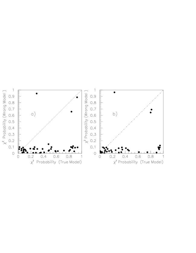
In this method, the distribution of some or all of the observed angular data is used directly in an unbinned maximum likelihood fit [7], in which parameters ${\bf P}$, denoting one or more of the Lagrangian contributions (4), are varied to maximize the quantity $$\ln{\cal L}_{ML}=\sum_{i}\ln p({\bf\Omega}_{i},{\bf P})-N_{obs}\ln\left\{\int p({\bf\Omega},{\bf P})d\Omega\right\},$$ (21) where the sum is over events in the sample, ${\bf\Omega_{i}}$ represents, for the i’th event, the angular information being used, $p({\bf\Omega},{\bf P})$ is derived from the cross-section (17), $N_{obs}$ is the observed number of events, and the integral is over the whole of phase space. Many of the results shown here have been obtained using the method of extended maximum likelihood, in which the absolute prediction for the magnitude of the cross-section is also tested [53]: $$\ln{\cal L}_{EML}=\sum_{i}\ln p({\bf\Omega}_{i},{\bf P})-N({\bf P}),$$ (22) where, for integrated luminosity $L$, the predicted number of events $N({\bf P})$ in the sample is $L\int\mbox{$\frac{{\mathrm{d}}\sigma}{{\mathrm{d}}{\bf\Omega}}$}({\bf\Omega},{\bf P}){\mathrm{d}}{\bf\Omega}$. It may be noted that, while in the evaluation of $N({\bf P})$ in (22) the absolute normalization of the cross-section must be used (as given in (17)), constant factors such as the flux factor may be omitted from the unnormalized expression $\int p({\bf\Omega},{\bf P})d\Omega$ in (21). Furthermore, since for any event the probability $p$ is proportional to the product of a phase space factor, which is independent of ${\bf P}$, and a matrix element squared, ${\mid{\cal M}\mid}^{2}$, which contains the dependence on the TGC parameters, the sums over events in (21) and (22) may be replaced by $\sum_{i}\ln{\mid{\cal M}\mid}^{2}({\bf\Omega}_{i},{\bf P})$, and the maximum of the likelihood function will be unchanged. While this replacement is trivial for the 2-body cross-section given by (12), it is essential in the evaluation of the log-likelihood sum when the reaction is analyzed in terms of the 4-fermion processes, in which the phase space factor is different for every event. While the maximum likelihood method is able to use all the available angular information for each event, it has the disadvantage compared with a $\chi^{2}$ fit of being unable to provide a goodness of fit criterion. Nonetheless, the goodness of fit of a hypothesis represented by the likelihood function ${\cal L}_{1}({\bf p})$ can be compared with that of ${\cal L}_{2}({\bf P})$ if the parameters ${\bf p}$ of ${\cal L}_{1}$ satisfy the condition ${\bf p}\in{\bf P}$. Then the quantity $-2\ln\left({\cal L}_{1}^{max}/{\cal L}_{2}^{max}\right)$, derived from the ratio of their likelihood functions, has a $\chi^{2}$ distribution [54]. This property has been applied to event samples generated with non-SM values of one TGC, $P_{1}$, and used to distinguish this hypothesis from a wrong one, when a different TGC, $P_{2}$, is fitted to the data. — In general, a fit of $P_{2}$ produces a result differing significantly from the SM value. Fig 6 shows the results of applying this test to the correct and wrong models in two alternative ways. In both cases, ${\cal L}_{1}$ is taken as the likelihood function when $P_{1}$ varies; in the “same family” case (a), ${\cal L}_{2}$ is the likelihood function when both $P_{1}$ and $P_{2}$ vary, while, in (b), ${\cal L}_{2}$ describes a “composite” hypothesis, $${\cal L}_{2}\left(P_{1},P_{2};\beta\right)=\prod_{i=1}^{N}\left[\beta p\left(P_{1}\right)+\left(1-\beta\right)p\left(P_{2}\right)\right],$$ (23) where $\beta$ is the probability that model 1, represented by the probability density function $p(P_{1})$, is correct, and $P_{1}$, $P_{2}$ and $\beta$ vary in the fit. It can be seen that a simple comparison between the values of these probabilities indicates the correct model for the majority of the cases. In addition, the absolute probability value indicates the goodness of the fit. Figure 6: Hypothesis testing using a) the “same family” and b) the “composite hypothesis” methods, for data sets of about 2500 $jj\ell\nu$ events generated with TGC values deviating from the SM values by one to five times the expected LEP2 precisions.

4.3 Optimal observables method

Optimal observables are quantities with maximal sensitivity  to the unknown coupling parameters [44, 56]. To construct them, a particular set of couplings $P_{i}$ is chosen which are zero at Born level in the Standard Model (for instance, the TGCs defined by (4)). Then, recalling that the amplitudes for the four-fermion process are linear in the couplings, the differential cross-section may be written $$\frac{{\mathrm{d}}\sigma}{{\mathrm{d}}{\bf\Omega}}=S_{0}({\bf\Omega})+\sum_{i}S_{1,i}({\bf\Omega})\,P_{i}+\sum_{i,j}S_{2,ij}({\bf\Omega})\,P_{i}P_{j}\;,$$ (24) where ${\bf\Omega}$ represents the kinematic variables as before. Kinematic ambiguities, such as those described in table 3, can readily be incorporated into (24). The distributions of the functions $${\cal O}_{i}({\bf\Omega})=\frac{S_{1,i}({\bf\Omega})}{S_{0}({\bf\Omega})}$$ (25) are measured, and their mean values $\langle{\cal O}_{i}\rangle$ evaluated. An example is shown in fig 7. To first order in the $P_{i}$, the mean values $\langle{\cal O}_{i}\rangle$ are given by $$\langle{\cal O}_{i}\rangle={\langle{\cal O}_{i}\rangle}_{0}+\sum_{j}c_{ij}\,P_{j}\;,$$ (26) from which the couplings $P_{j}$ can be extracted because ${\langle{\cal O}_{i}\rangle}_{0}$ and $c_{ij}$ are calculable given (24) and (25). From the distributions of the ${\cal O}_{i}$ the statistical errors on their mean values can be evaluated, the observables having been constructed to minimize the induced errors on the $P_{j}$. If the linear expansion in the couplings is good, the method has the same statistical sensitivity as a maximum likelihood fit. It can also be extended to incorporate total cross-section information in a manner analogous to the use of the extended maximum likelihood method discussed in the previous section. Figure 7: Distribution of ${\cal O}_{\mbox{$\alpha_{W\phi}$}}(\mbox{$\cos\theta$},(\mbox{$\cos\theta_{l}$},\mbox{$\phi_{l}$}),(\mbox{$\cos\theta_{j}$},\mbox{$\phi_{j}$})\mbox{${}_{\mathrm{folded}}$})$ for a large sample (50000) of simulated $\mbox{$e^{+}e^{-}$}\rightarrow\mbox{$W^{+}W^{-}$}$ events at 190 GeV. The experimentally determined mean value is to be compared with the expectation value of this observable in the SM, $\mbox{$\alpha_{W\phi}$}=0$, used to generate the events.

4.4 Comparison of methods

In this section a comparison is presented of fits of the TGCs $\alpha_{W\phi}$, $\alpha_{B\phi}$ and $\alpha_{W}$, defined in (4), to common datasets generated with the PYTHIA[57] Monte Carlo simulation program. We precede this by mentioning the results of a comparison of the use of the maximum and extended maximum likelihood (ML and EML) methods, in which both of these methods were used in fits of the three TGCs to a large sample (50000) of events using first only the $W$ production angle, and then the complete angular information (production and decay angles). The extra information contained in the EML method gave a substantial improvement (10%) in precision only in one case — the fit of $\alpha_{B\phi}$, generally the least well determined parameter, to the production angular distribution. In the other fits the improvement was only $\sim 1\%$. Similar conclusions have been obtained when applying the optimal observables method with and without total cross-section information. In the comparison of the density matrix (DM), EML and optimal observables (OO) methods, the three analyses were applied to datasets at 175 and 190 GeV simulating both the expected LEP2 statistics ($\approx$ 2000 events) and much larger statistics (50000 events). Sample results are given in fig 8, in which precisions obtained using the three methods in 1- and 2-parameter fits to the large dataset at 190 GeV are plotted. In all cases, the precisions obtained using the three methods are very similar when the same angular data is used in the fit. This can be seen in the figure, where the precisions from the EML and OO methods, both of which used angular data $\cos\theta$, ($\cos\theta_{l}$, $\phi_{l}$) and ($\cos\theta_{j}$, $\phi_{j}$)${}_{\mathrm{folded}}$, are almost identical. The DM results shown used the differential cross-section, $\frac{{\mathrm{d}}\sigma}{{\mathrm{d}}\!\cos\theta}$, density matrix elements $\rho_{00},\rho_{1\!-1},\rho_{1\!0}$ and $\rho_{-1\!0}$ of the leptonically decaying $W$, and the part symmetric in both polar decay angles of the transverse element $\rho_{TT}\equiv\rho_{11,11}+\rho_{-1\!-1,-1\!-1}+\rho_{11,-1\!-1}+\rho_{-1\!-1,11}$ of the joint $WW$ density matrix, representing somewhat less than the full 35 (CP-conserving) elements of the full joint density matrix. (Other density matrix elements can in principle be included in the analysis). Figure 8: Comparison of TGC fits to a large sample of simulated events at 190 GeV using the density matrix (DM), maximum likelihood (EML) and optimal observables (OO) methods. a): 1 s.d. precisions in 1-parameter fits to $\alpha_{W}$, $\alpha_{W\phi}$ and $\alpha_{B\phi}$.  b): 95% confidence contours in 2-parameter fits to ($\alpha_{W\phi}$, $\alpha_{B\phi}$). A difference between the EML or DM analyses and the OO analysis can be seen in the 2-parameter fit shown, where a second allowed region, remote from the SM region $(\mbox{$\alpha_{W\phi}$}=0,\mbox{$\alpha_{B\phi}$}=0)$ where the events were generated, is seen by the EML and DM methods. This effect is discussed in detail in ref. [7], where it is shown to arise naturally from the amplitude structure of $WW$ production, and in particular from the fact that the helicity amplitudes are linear in the TGCs. It is not seen in the OO results, because here the cross-section (24) has been linearized with respect to the TGCs about their SM values. In considering possible extensions to the analyses, two comments may be made. First, the EML and OO methods could readily be used in a 4-fermion treatment by replacement of the matrix elements. The DM method does not lend itself to this adaptation, as the form (17) used in the projection of the density matrix elements assumes $J=1$ for the two final state $f\bar{f}$ pairs. Second, all three methods can in principle be adapted to the analysis of events with the experimental and other effects discussed later in this chapter; however, we have not made an assessment of the relative ease with which this can be done for the different methods. With the above points borne in mind, we can recommend all three methods for consideration in the analysis of LEP2 data. The studies reported in the following sections have, except where otherwise indicated, used ML or EML fits to obtain the results shown.

5 Precision of TGC determination at LEP2: generator level studies

In this section, the precisions to be expected in TGC determination from the anticipated LEP2 integrated luminosity are summarized and an estimate of the biases and systematic errors accessible at generator level is given.

5.1 TGC precisions in fits to simulated events

Precisions in TGCs obtained from 1-parameter fits to simulated $\mbox{$e^{+}e^{-}$}\rightarrow\mbox{$W^{+}W^{-}$}$events at 176 and 190 GeV are shown in table 5, and confidence limits in the planes of two of the three possible combinations of two of the parameters in eq. (4) are shown in fig 9. Results are shown using various combinations of the angular data appropriate to each of the three final states $jj\ell\nu$, $jjjj$ and $\ell\nu\ell\nu$, as indicated in table 3, as well as to the “ideal” case without angular ambiguities. For the first two channels (and for the “ideal” analysis), 1960 (2600) events were fitted at 176 (190) GeV; for the $\ell\nu\ell\nu$ channel, 280 (370) events were used. These figures emulate the statistics anticipated from an integrated luminosity of $500{\mathrm{p}b}^{-1}$ after experimental efficiency cuts of $\sim 95\%$, 60% and 95% for the three channels respectively, and excluding leptonic decays into $\tau\nu_{\tau}$. The extended maximum likelihood method was used in the fits, and the events were generated and analyzed in the narrow $W$ width approximation and without initial state radiation (ISR). In the analysis, the generated values of parton momenta were used, so that no account has been taken of the subsequent quark fragmentation nor of possible experimental effects. No kinematic cuts have been made on the data. The analysis reported here is therefore to be considered as an idealized one; the implications of the additional effects mentioned above are considered in detail in subsequent sections. Several conclusions may be drawn from inspection of the table and figure. As anticipated by the discussion of section 3, substantial gains in precision are achievable by running at higher energy. Also, use of as much as possible of the available angular data serves to increase the precision and, in 2-parameter fits, to reduce the (quite pronounced) correlations between the fitted TGCs. The use of the $jjjj$ channel, even with the angular ambiguities incurred by the inability to distinguish quark from antiquark jets, can be seen to provide a modest but worthwhile improvement in the overall precision attainable. Finally, the occurrence of a second region in the ($\alpha_{W\phi}$, $\alpha_{B\phi}$) plane, remote from the Standard Model region ($0,0$) at which the events were generated but acceptable at the chosen significance level, has already been noted in the previous section. Model Channel Angular data used 176 GeV 190 GeV $\alpha_{B\phi}$ $jj\ell\nu$ $\cos\theta$ 0.222 0.109 $\cos\theta$, ($\cos\theta_{l}$, $\phi_{l}$) 0.182 0.082 $\cos\theta$, ($\cos\theta_{l}$, $\phi_{l}$), ($\cos\theta_{j}$, $\phi_{j}$)${}_{\mathrm{folded}}$ 0.159 0.080 $jjjj$ $\mid\mbox{$\cos\theta$}\mid$ 0.376 0.149 $\mid\mbox{$\cos\theta$}\mid$, ($\cos\theta_{j_{1}}$, $\phi_{j_{1}}$)${}_{\mathrm{folded}}$, ($\cos\theta_{j_{2}}$, $\phi_{j_{2}}$)${}_{\mathrm{folded}}$ 0.328 0.123 $\ell\nu\ell\nu$ $\cos\theta$, ($\cos\theta_{1}$, $\phi_{1}$), ($\cos\theta_{2}$, $\phi_{2}$), 2 solutions 0.323 0.188 Ideal $\cos\theta$, ($\cos\theta_{1}$, $\phi_{1}$), ($\cos\theta_{2}$, $\phi_{2}$) 0.099 0.061 $\alpha_{W\phi}$ $jj\ell\nu$ $\cos\theta$ 0.041 0.027 $\cos\theta$, ($\cos\theta_{l}$, $\phi_{l}$) 0.037 0.023 $\cos\theta$, ($\cos\theta_{l}$, $\phi_{l}$), ($\cos\theta_{j}$, $\phi_{j}$)${}_{\mathrm{folded}}$ 0.034 0.022 $jjjj$ $\mid\mbox{$\cos\theta$}\mid$ 0.098 0.054 $\mid\mbox{$\cos\theta$}\mid$, ($\cos\theta_{j_{1}}$, $\phi_{j_{1}}$)${}_{\mathrm{folded}}$, ($\cos\theta_{j_{2}}$, $\phi_{j_{2}}$)${}_{\mathrm{folded}}$ 0.069 0.042 $\ell\nu\ell\nu$ $\cos\theta$, ($\cos\theta_{1}$, $\phi_{1}$), ($\cos\theta_{2}$, $\phi_{2}$), 2 solutions 0.096 0.064 Ideal $\cos\theta$, ($\cos\theta_{1}$, $\phi_{1}$), ($\cos\theta_{2}$, $\phi_{2}$) 0.028 0.018 $\alpha_{W}$ $jj\ell\nu$ $\cos\theta$ 0.074 0.046 $\cos\theta$, ($\cos\theta_{l}$, $\phi_{l}$) 0.062 0.038 $\cos\theta$, ($\cos\theta_{l}$, $\phi_{l}$), ($\cos\theta_{j}$, $\phi_{j}$)${}_{\mathrm{folded}}$ 0.055 0.032 $jjjj$ $\mid\mbox{$\cos\theta$}\mid$ 0.188 0.110 $\mid\mbox{$\cos\theta$}\mid$, ($\cos\theta_{j_{1}}$, $\phi_{j_{1}}$)${}_{\mathrm{folded}}$, ($\cos\theta_{j_{2}}$, $\phi_{j_{2}}$)${}_{\mathrm{folded}}$ 0.131 0.069 $\ell\nu\ell\nu$ $\cos\theta$, ($\cos\theta_{1}$, $\phi_{1}$), ($\cos\theta_{2}$, $\phi_{2}$), 2 solutions 0.100 0.064 Ideal $\cos\theta$, ($\cos\theta_{1}$, $\phi_{1}$), ($\cos\theta_{2}$, $\phi_{2}$) 0.037 0.022 Table 5: 1 s.d. errors in fits of $\alpha_{B\phi}$, $\alpha_{W\phi}$ and $\alpha_{W}$ to various combinations of the angular data at 176 and 190 GeV. The simulated data corresponds to integrated luminosity of $500{\mathrm{p}b}^{-1}$. Details of the data samples are given in the text. Figure 9: 95% confidence limits in the planes of 2-parameter TGC fits at 176 and 190 GeV, using various combinations of angular data. a), b), c), d): Fits to ($\alpha_{W\phi}$, $\alpha_{B\phi}$); e), f), g), h): Fits to ($\alpha_{W\phi}$, $\alpha_{W}$). In the legend, the notation $\Theta_{l,j}$ implies a pair of decay angles $(\theta_{l,j},\phi_{l,j})$ for $W\rightarrow$ (leptons, jets) respectively, and $\mid\Theta_{j}\mid$ implies the ambiguity $\mbox{$\cos\theta_{j}$}\leftrightarrow-\mbox{$\cos\theta_{j}$}$, $\mbox{$\phi_{j}$}\leftrightarrow\mbox{$\phi_{j}$}+\pi$ incurred by the inability to distinguish quark from antiquark jets. In plots a), b), e), f), the angular data simulates channel $jj\ell\nu$ (and the “ideal” case, with no ambiguities); in c), d), g), h), it simulates channel $jjjj$. In a first step towards a more realistic simulation of the data, some of the fits described above have been repeated using calculations corresponding to 4-fermion rather than $WW$ production both in event generation and analysis. In so doing, contributions are included from the complete set of relevant diagrams and the finite $W$ width effects ignored in the previous analysis are taken into account. Using events generated with the ERATO [46] program corresponding to the expected statistics at 175 and 190 GeV, similar precisions to those shown above are obtained in fits of $\alpha_{W\phi}$ and $\alpha_{W}$ to angular data $\cos\theta$, ($\cos\theta_{l}$, $\phi_{l}$) and ($\cos\theta_{j}$, $\phi_{j}$)${}_{\mathrm{folded}}$. In addition, in fits to a sample of $jj\ell\nu$ events generated at 161 GeV corresponding to an integrated luminosity of $100{\mathrm{p}b}^{-1}$ (as suggested for the determination of the $W$ mass from its threshold excitation [58]), 1 s.d. precisions of 0.18 and 0.43 were obtained in fits of $\alpha_{W\phi}$ and $\alpha_{W}$ respectively. It is interesting to note that these values compare well with current experimental limits [25, 26], implying that TGC measurements from this exposure may also be of interest. This conclusion, however, remains to be tested when backgrounds and other experimental effects are included.

5.2 Biases and systematic errors in TGC determination calculable at generator level

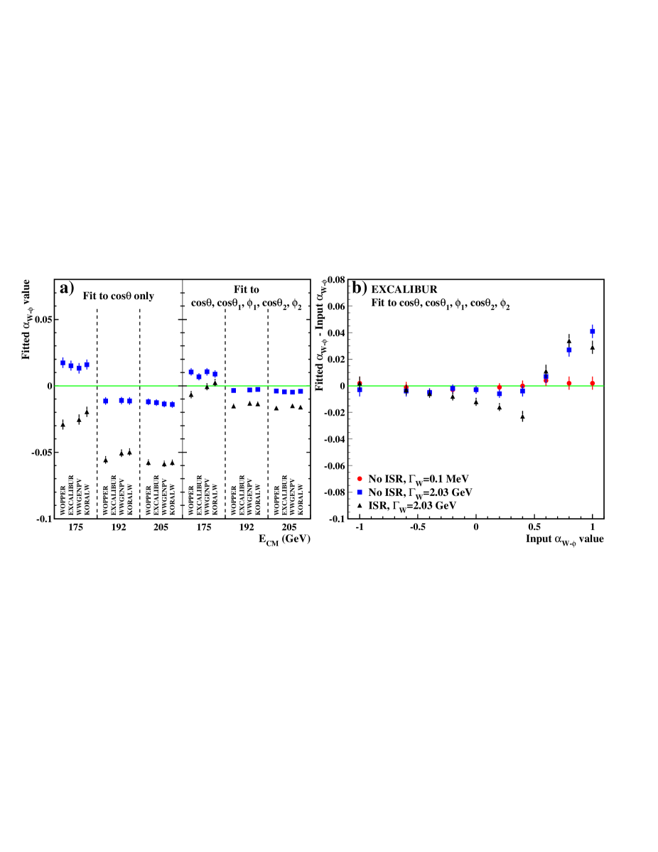
It was pointed out in the previous section that the analyses presented there are idealized, in the sense that effects due to finite $W$ width (unless a 4-fermion calculation is used), ISR, QCD and experimental reconstruction have been ignored. In this section, we consider the biases introduced in TGC determinations, first, if events generated with a realistic $W$ mass distribution are nonetheless analyzed in the narrow width approximation, and, second, if ISR effects are also present, but ignored in the analysis. The discussion of the overall bias to be expected in TGC determination is pursued in the next section, where biases arising due to event selection and reconstruction are added to those discussed here. The systematic errors incurred both in the assessment of these biases and from other sources calculable at generator level are also estimated in this section. Figs. 10a) and b) show the effects of ignoring finite $W$ width and ISR in the analysis of events generated with these effects included. Results are shown for several different generators, all operating in $\mbox{$e^{+}e^{-}$}\rightarrow\mbox{$W^{+}W^{-}$}$ (CC03) mode. It can be seen, first, that the bias incurred by neglect of ISR is greater than that from neglect of $W$ width effects, second, that the biases are smaller when a fit involving more angular data is used, and, third (from b), that the biases are different for different values of a typical TGC parameter. Finally, we note that the overall bias is $\lesssim$ the statistical error expected from LEP2 data. Figure 10: Effect of ignoring finite $W$ width and ISR in TGC fits. a): Results of fits of $\alpha_{W\phi}$ to events generated with SM parameters at three energies using various generators. Left-hand plots: fit to $\cos\theta$ only; Right-hand plots: fit to $\cos\theta$, ($\cos\theta_{1}$, $\phi_{1}$), ($\cos\theta_{2}$, $\phi_{2}$). b): as a), for EXCALIBUR events at 190 GeV, using $\cos\theta$, ($\cos\theta_{1}$, $\phi_{1}$), ($\cos\theta_{2}$, $\phi_{2}$), as a function of $\alpha_{W\phi}$. The legend for both plots is shown on b). The systematic errors arising from these and other sources calculable at generator level are summarized, using a particular TGC fit as an example, in table 6. The first three entries come from the effects discussed above, the next two represent two different ways of expressing the uncertainty in the other electroweak parameters which are important in the evaluation of the matrix element, and the final pair represent two independent uncertainties coming from machine and detector considerations. In any analysis which does not compare total cross-section predictions with the observed data, the second and last entries will not contribute to the overall uncertainty. It can be seen that, even when all the relevant entries are added in quadrature, the total is small compared with the statistical precision expected from LEP2 data, and we expect the larger component of the systematic error to come from uncertainties in the experimental effects considered in the next sections. Source of uncertainty Uncertainty Systematic error in $\alpha_{W\phi}$ $W$ width $\Delta\Gamma_{W}=\pm 0.07$ GeV $\pm 0.0004$ ISR $\Delta\sigma_{tot}/\sigma_{tot}(\mbox{$\mbox{$e^{+}e^{-}$}\rightarrow\mbox{$W^{+}W^{-}$}$}+radiation)=\pm 1\%$ $\pm 0.0013$ ISR parametrization Spread in Monte Carlo estimates $\pm 0.0020$ $M_{W}$ $\Delta M_{W}=\pm 0.18$ GeV $\mp 0.0021$ $\sin^{2}\theta_{W}$ $\sin^{2}\theta_{W}=0.226$ (tree-level) $\rightarrow\sin^{2}\theta_{W}=0.231$ 0.0029 Beam energy $\Delta\sqrt{s}=\pm 15$ MeV $\mp 0.0002$ Absolute normalization $\pm 1\%$ $\pm 0.0013$ Table 6: Systematic errors from various sources incurred in fits of $\alpha_{W\phi}$ to angular data $\cos\theta$, ($\cos\theta_{l}$, $\phi_{l}$), ($\cos\theta_{j}$, $\phi_{j}$)${}_{\mathrm{folded}}$ at 190 GeV. The 1 s.d. statistical precision estimate for this fit from LEP2 data (c.f. table 5) is $\pm 0.022$. In addition to the effects considered above, it is legitimate to ask whether colour recombination effects among the two $W$s could affect TGC measurements in the $jjjj$ channel. It has recently been advocated that such effects may produce a shift of up to 400 MeV in $M_{W}$ [59]. Therefore, by analogy with the effects of ISR, it may produce a bias in TGC measurements which would need to be accounted for, and, if not understood, would have an associated systematic error. However, a preliminary study [60] has indicated that the $W$ production angular distribution, reconstructed from the hadronization products of generated $jjjj$ events, is little affected by application of the colour recombination models of ref [59], and hence that it is unlikely that the shift in TGC values determined from the data in this channel will be significant compared to the expected statistical error.

6 Analysis of the $jje\nu$ and $jj\mu\nu$ final states

In the following we address some of the experimental aspects of the analysis of the $e^{+}e^{-}\rightarrow W^{+}W^{-}\rightarrow\mbox{$jj\ell\nu$}$ channel. In this section, we concentrate on the muon and electron channels, these being the cleanest and very similar in many respects. The tau channel is considered separately in the following section. For simplicity, the data are analyzed in terms of the five angles describing $WW$ production and decay, by analogy with the generator-level analysis reported in section 5.1. In its extension to a four-fermion treatment, also described in that section, the effect of the experimental selection and reconstruction procedures are expected to be the same. In section 6.1 we describe the efficiencies and purities obtained after the application of typical selection criteria and of kinematic constraints to the events. In the process of reconstructing and analyzing $jj\ell\nu$ events, there are many experimental effects which can potentially bias the angular distributions, and hence the fitted values of TGC parameters. The scale of such effects is estimated in section 6.2, and in section 6.3 we discuss briefly some methods proposed to allow for them in the analysis. The numbers presented result from a comparison of the work of several different groups and should be regarded as broadly typical of the four LEP experiments.

6.1 Event selection, kinematic reconstruction and residual background

The $jj\ell\nu$ event selections used typically demand the following: - that the event contains a minimum number, typically five or six, of charged track clusters; - that there is an identified electron or muon, or alternatively a high energy isolated track; - that the lepton has a momentum greater than its kinematic minimum, $\sim 20$ GeV; - that the lepton be isolated, by requiring low activity in a cone around the track (typically that the energy deposited in a cone of 100-200 mrad be less than 1-2 GeV). The effect of these cuts corresponds approximately to a fiducial cut in the centre-of-mass polar angle of the lepton of $|\cos\theta_{lepton}|<0.95$. The acceptance for jets, which have some angular size, extends further but with falling efficiency. These numbers vary for specific detectors. The non-lepton system is then split into two (or more) jets using a conventional jet-finding algorithm. The following kinematic constraints [61] can then be applied to impose energy and momentum conservation, and to improve the measurements using the fact that the system is overconstrained: 1C fit:   $\sum E=E_{cm}$, $\sum\vec{p}=0$, $m_{\nu}=0$; 3C fit:   In addition to 1C, $M_{reconstructed}=M_{W}$ for both $W$ candidates; 3C${}^{\prime}$ fit:   In addition to 1C, $M_{reconstructed}$ for both $W$  candidates is constrained to a central value of $M_{W}$ but is allowed to vary approximately within the $W$ width. In the above, $m_{\nu}$ is the neutrino mass and $M_{W}$ the $W$ mass. A $\chi^{2}$ probability cut, typically of 0.1-1%, is applied to the constrained fit result. Typical efficiencies after these stages are shown in table 7 for centre-of-mass energies $\sqrt{s}=175$ and $192$ GeV. The main loss is due to geometrical acceptance and lepton identification in the basic selection. The kinematic fits themselves are of the order of 90% efficient for such a probability cut. Efficiency % Background % $Z\gamma$ $WW$ (non-$jj\ell\nu$) $ZZ$ Total $E_{cm}$ = 175 GeV Basic Selection 77 8 6 1 15 1C fit 75 7 5 1 13 3C fit 70 1 2 0.5 3.5 3C${}^{\prime}$ fit 72 1 4 0.5 5.5 $E_{cm}$ = 192 GeV Basic Selection 75 7 8 2 17 1C fit 73 6 7 2 15 3C fit 66 1 2 1 4 3C${}^{\prime}$ fit 71 1 3 1 5 Table 7: Efficiencies and purities of the $jj\ell\nu$ sample at progressive stages of selection and kinematic fitting. The background estimation was made using event samples, simulated with PYTHIA, of the final states $WW$ (with neither of the bosons decaying to an electron or a muon), $Z\gamma$, $ZZ$ and $Zee$. Also, contamination from $\gamma\gamma$ events, generated with TWOGAM [62], were studied. Backgrounds from the last two channels were found to be negligible; those from the other final states are summarized in table 7. Contributions from the non-resonant graphs leading to the $jj\ell\nu$ final state and containing TGCs have also been studied. It is found that, taken in isolation and ignoring interferences, they are rejected by the selection procedure. The main contribution to the $WW$ background comes from events where one of the $W$s  decays into a tau and then into an electron or muon. Although this channel is sensitive to the TGCs, it will be seen in section 6.2 that the inclusion of such events into the analysis does not significantly bias the result. Other approaches can be used instead of the selection procedure described above . In particular, if one wishes to avoid the use of the constrained fit, a cut requiring the missing momentum direction to be away from the beam pipe, typically $\cos\theta<0.95$, can be used to reduce the background from the $ZZ$ and $Z\gamma$ channels. In this case, an algorithm has to be applied to impose energy and momentum conservation. Nonetheless, in the rest of this section we adopt the 3C fits as representative of the efficiency and purity which can be achieved. The resolutions obtained for the $WW$ production and decay angles before and after kinematic fitting are shown in table 8. The values shown are averages over the whole fiducial region; however, in general, the resolutions depend upon the values of the kinematic variables themselves and, following kinematic fitting, they are correlated. It can be seen that a modest improvement in resolution is obtained, the main qualitative effect being due to the recovery of mis-measured events. Selection Resolution $\cos\theta$ $\cos\theta_{l}$ $\phi_{l}$ (rad) $\cos\theta_{j}$ $\phi_{j}$ (rad) Before fit 0.06-0.13 0.11-0.17 0.12-0.23 0.13-0.19 0.11-0.22 After 3C${}^{\prime}$ fit 0.05-0.12 0.07-0.13 0.10-0.21 0.10-0.17 0.11-0.21 Table 8: Resolutions on $WW$ production and decay angles using simulated events at 192 GeV. The ranges indicate the spread of values obtained from different experimental simulations.

6.2 Systematic biases and statistical precision

We now consider potential systematic biases, and the degradation of statistical precision due to experimental effects in the $jj\ell\nu$ channel. In this we include a) the neglect of ISR and $\Gamma_{W}$, b) experimental acceptance, c) reconstruction and detector resolution, and d) residual background contamination. The first item has been discussed in detail in section 5.2; the result is included here for completeness. We use as example fits to $\alpha_{W\phi}$ only. The overall bias due to a)-d) has been determined using a total of approximately 20,000 simulated $jj\ell\nu$ events at 175 GeV and 30,000 events at 192 GeV. A maximum likelihood or extended maximum likelihood fit was used, assuming in the analysis that the events originate from $WW$  production with narrow $W$ width and without initial state radiation. We emphasize that, since the purpose of this study is to show explicitly the scale of the biases, no corrections for the effects listed above have been applied in the analysis. 175 GeV 192 GeV 1-D 5-D 1-D 5-D Statistical Precision $\pm 0.041$ $\pm 0.034$ $\pm 0.027$ $\pm 0.022$ (from table 5) Biases to Measurement:   ISR and $\Gamma_{W}$ $-0.03$ $-0.01$ $-0.05$ $-0.02$   Selection/Acceptance $-0.06$ $-0.02$ $-0.03$ $-0.03$   Reconstruction/resoln. $-0.05$ $-0.01$ $-0.03$ $-0.01$ Total $-0.14$ $-0.04$ $-0.11$ $-0.06$ Approximate additional bias due to backgrounds   $WW$ $-0.005$ $-0.002$ $-0.003$ $-0.002$   $Z\gamma$ $+0.003$ $+0.008$ $-0.003$ $+0.002$   $ZZ$ $-0.003$ $-0.001$ $-0.012$ $-0.002$ Table 9: Biases in the measurement of $\alpha_{W\phi}$ estimated from studies of large samples of fully simulated events. In the last part of the table the additional biases due to residual backgrounds are shown. The results are shown in table 9. The column labelled 1D refers to fits using only the production angle $\cos\theta$. The column labelled 5D refers to fits using the production and decay angles (with the angles of the hadronically decaying $W$ folded to take account of the ambiguity described in table 3). The bias due to ISR and $\Gamma_{W}$ is derived as described earlier. The bias due to event selection and acceptance was determined by comparing fits to the generated angles before and after event selection, and the bias due to reconstruction and resolution was determined by comparing fits to generated angles with fits to fully reconstructed angles. In the last part of the table the additional biases due to background are shown. However the reader should be aware that these were measured by adding small numbers of events to the sample, and in the absence of a systematic study should be considered to be very approximate. We conclude that the size of the biases from ISR and $\Gamma_{W}$, acceptance and reconstruction are up to a few times the expected statistical error in the case of 1D fits, and somewhat smaller when all the angular information is used. In order that these effects do not present a serious source of systematic error compared to the statistical error, they will eventually have to be understood and corrected for, incurring an error of less than $\sim 10\%$ of their values. Finally, we investigate the extent to which the statistical precision in TGC determination is degraded due to the effects mentioned above. The large simulated sample was divided into subsamples corresponding to the expected LEP2 statistics. The TGC parameter fit was performed on each sample, and the standard deviation of the spread of the results calculated. The precisions given for fits to generator level data for the $jj\ell\nu$ channel in table 5 assume an efficiency of 95%; thus the ideal precision in this channel is better by a factor $\sqrt{0.95}=0.97$. Taking this and the estimated experimental efficiency of 70% shown in table 7 into account, we expect a statistical degradation of $\sim\pm 20$% with respect to this ideal case. This is indeed observed, together with an additional degradation of $\pm 10$% to $\pm 20$% after application of the analysis procedure described above, showing the effect of the extra randomization from ISR, $\Gamma_{W}$ and experimental effects.

6.3 Strategies for allowing for systematic biases

In the previous section the scale of the potential systematic bias due to detector and other effects was quantified. The simplest method of correction for such a bias is to determine its value for many simulated samples, subtract the mean bias from the experimentally measured TGC value and assign a systematic error on the basis of the width of the bias distribution and the experimental number of events. If the spread on the bias is large compared with the statistical error, this procedure will clearly be far from optimal. A second method is to use a Monte Carlo simulation to produce a correction function to map between “true” and “measured” values. This can easily be applied when fitting to a small number of variables, for instance to the $\cos\theta$ distribution alone, but is more difficult to apply in 5 dimensions simply because of the number of events required to characterize a 5D function in several bins per variable (unless corrections for each variable can be assumed to factorize). It has previously been shown at generator level that the precision is maximized by using all variables; it may however be that when systematic errors are taken into account the best overall precision is obtained by using a different strategy. It is nonetheless possible to formulate methods which take resolution effects into account in fits using all the kinematic variables. For instance, if the resolution/acceptance function for the variables ${\bf\Omega}$ is known, then the probability function $p({\bf\Omega},{\bf P})$ used for each event in the maximum likelihood expressions (21) and (22) given in section 4.2 can be replaced by $$p_{eff}({\bf\Omega}_{meas},{\bf P})=\int p({\bf\Omega}_{true},{\bf P})\times\rho({\bf\Omega}_{true}\rightarrow{\bf\Omega}_{meas}){\mathrm{d}}{\bf\Omega}_{true}$$ (27) (where ${\bf P}$ represents the TGC parameters of the fit). The resolution/acceptance function $\rho$ gives the probability that the true value ${\bf\Omega}_{true}$ would be reconstructed as ${\bf\Omega}_{meas}$. There are several potential problems with the application of (27): (i) a 5-D integration is required; (ii) the resolution and acceptance functions will almost certainly not be simple, nor will they factorize; (iii) the correlations between angles must be known and included (in particular if kinematically fitted quantities are used). One suggested method [63] uses fully simulated Monte Carlo events which are passed through the same events selection as data, in order to calculate the effective likelihood function. The variation of the TGC parameters is performed by reweighting the Monte Carlo events at their generated coordinates, while the comparison with data is performed at the reconstructed coordinates. This method can be applied for any fit dimension and can in principle take into account the effect of acceptance cuts, experimental resolution, any kinematic fitting procedure and background contamination in the data.

7 Analysis of the $jj\tau\nu$ final state

This channel requires special attention for two reasons. First, it comprises a sizeable part of the semileptonic $WW$ decays and therefore could provide a useful addition to the available statistics and, second, it is a background mainly for the hadronic channel and therefore methods are required to reject it. In this study we consider only the hadronic decays of the $\tau$ and describe criteria to select this final state. The resulting efficiency and purity expected for the sample and the resolution expected in the angular variables are presented. We find that an increase in the overall number of events selected for analysis in the $jj\ell\nu$ channel of between $10-20\%$ can be expected.

7.1 Selection and reconstruction of $jj\tau\nu$ events

To select $jj\tau\nu$ events, we make use of the characteristics of the $\tau$ jet, namely small jet opening angle and low jet-charge multiplicity and of the global characteristics of the event, mainly missing energy and event acoplanarity. The signal for the $jj\tau\nu$ final state has a 3-jet topology, while the main sources of background ($\mbox{$WW$}\rightarrow\mbox{$jjjj$}$ and $\mbox{$WW$}\rightarrow Z\gamma(s)\rightarrow q\bar{q}\gamma$) fall into the 4-jet and 2-jet topologies respectively. Thus the choice of the resolution parameter in a jet-clustering algorithm is quite significant. Requiring at least 3 jets in the event, we find a $\tau$-reconstruction efficiency of $70-80\%$ while only $30-40\%$ of $Z\gamma$ events survive. The clustering algorithm itself ensures isolation for the $\tau$ jet. Jets from $\tau$ decays can be distinguished from quark and gluon jets by the distribution of quantities such as the track multiplicity (total or charged), the maximum angle of any charged track in the jet to the jet axis, and the fractional energy of the jet contained within a cone of a specified angle (say, 0.1 rad) about the jet axis. A likelihood function based on such parameters has been constructed, giving a typical efficiency of about $70\%$ with a rejection factor for quark and gluon jets close to 50. The charge of the $\tau$ lepton can be estimated rather reliably from the total charge of the tracks in the jet (excluding those with momenta $<$ 1 GeV/c from the sum in order to reduce the contribution from soft tracks from neighbouring jets). The $\tau$ signal can be further enhanced by requiring that the event contains less than five jets and that the sum of the missing energy and the energy of the reconstructed $\tau$ candidate should exceed $\sqrt{s}/2$. This results in a selection efficiency for $\tau$ events of about 90% with a rejection factor against the $WW$ $\rightarrow$ $jjjj$ channel and against $ZZ$ events of greater than 10. In addition, constraints on the polar angle of the missing momentum and the acoplanarity of the event can be imposed to reduce further the background from $Z\gamma$ events. A rejection factor of 10 is obtained while about $20\%$ of the signal is lost. Finally, the very forward electromagnetic calorimetry can be used to detect ISR photon(s) in cases where they have not escaped in the beam pipe. It may be noted from the above that missing energy and missing momentum are key variables for the rejection of all types of background, and therefore the hermiticity of the detector is an important factor. The efficiencies and purities obtained for $jj\tau\nu$ events from a sample of simulated events at 192 GeV are shown in table 10. The background from the $jj\ell\nu$ channel stems mainly from inefficiencies in muon detection in the simulation used, and some improvement may be possible here. The application of a 2-constraint kinematic fit can also be seen to provide background rejection, with a small decrease in the $\tau$ selection efficiency. Selection Efficiency % Background % $Z\gamma$ $WW\rightarrow\mbox{$jjjj$}$ $WW\rightarrow\mbox{$jj\ell\nu$}$ $ZZ$ total No fit 35 - 45 4 - 6 4 - 8 5 - 8 0 - 2 13 - 24 2C fit 32 - 42 0 - 2 2 - 5 5 - 8 0 - 0 7 - 15 Table 10: Typical efficiencies and purities for the $jj\tau\nu$ channel with no kinematic fit and with a 2-constraint kinematic fit. An improvement to the kinematic fit may result by constraining the $\tau$ momentum, using the fact that the direction of the $\tau$ can be accurately estimated from the combined momentum of its visible decay products, so that the $\tau$ energy can then be computed from the $W$ decay kinematics [64].

7.2 Resolution in reconstructed quantities

The resolution in the centre-of-mass polar and azimuthal angular variables of the $\tau$, evaluated using 2-Gaussian fits to the differences between reconstructed and generated values, is of the order of 5 mrad in 75% of the events, and is not changed much by the kinematic fit. The energy of the original $\tau$ can only be estimated at a level of $\Delta E/E=0.15$ with no kinematic fit, but after the fit has a resolution $\Delta E/E=0.05$ in 80% of events. The resolutions in the $W$ production and decay angles, evaluated after the kinematic fit, are found to be $\Delta cos\theta=0.11$, $\Delta cos\theta_{\tau}=0.13$ and $\Delta\phi_{\tau}=250$ mrad respectively.

7.3 TGC determination from $jj\tau\nu$ events

The precision with which TGCs can be determined from $jj\tau\nu$ events has been investigated using a sample of 937 fully simulated events, generated at 192 GeV with finite $W$ width and ISR, corresponding to an integrated luminosity of $500{\mathrm{p}b}^{-1}$. Of these events, 390 survived the selection and reconstruction procedures described above. The parameter $\alpha_{W\phi}$ was fitted to the cross-section (17) (i.e. in the narrow width, no ISR approximation), using the extended maximum likelihood method described in section 4.2 and folding over the 2 ambiguous solutions. The 1 s.d. precision in $\alpha_{W\phi}$  was found to be $\pm 0.06$ with estimated biases of $-0.04$ from the neglect of $W$ width and ISR, $-0.025$ from the effects of reconstruction, and $+0.03$ from the presence of background events.

8 Analysis of the $jjjj$ final state

The advantage of the high branching fraction of this channel is somewhat reduced by experimental difficulties associated with the purely hadronic nature of the final state. Background rejection in the four-jet channel is difficult, since no high-energy charged lepton is present to tag one $W$ as in the semileptonic case. The largest background is expected from the high cross-section channel $\mathrm{e^{+}e^{-}\rightarrow Z/\gamma^{*}\rightarrow q\bar{q}(\gamma)}$ leading to multi-jet final states. Also, since the decay modes of the two $W$s are both hadronic, the problem arises of selecting the correct pairs of jets to form the two $W$s and of assigning their charges. In the following we suggest an analysis of the $jjjj$ channel, including event selection, jet reconstruction and kinematic fitting, and indicate the expected efficiency and background levels. A section is devoted to jet- and W-charge tagging. We then discuss the determination of TGCs from the selected events, and draw conclusions on the sensitivity of the four-jet channel.

8.1 Selection of events and reconstruction of 4 jets in the final state

The general criteria for the selection of $jjjj$ events are based on the fact that the hadronization of four quarks gives rise to a high multiplicity of particles in the final state, and to a large visible energy. Other types of events with hadrons in the final state can have similar characteristics, mainly the $jj\ell\nu$ channel and the reactions $e^{+}e^{-}\rightarrow q\overline{q}\gamma$ with $M_{q\overline{q}}>$120 GeV and $e^{+}e^{-}\rightarrow\mbox{$ZZ$}\rightarrow q\overline{q}q^{\prime}\overline{q}^{\prime}$. The first two reactions can mimic 4 jets when gluon radiation has occurred. The following variables were typically used to select $jjjj$ events: - A large multiplicity of particles in the detector ($N_{charged}>25$, or $N_{charged}+N_{neutr}>25-40$). This cut helps to reject $jj\ell\nu$  and QCD background, where the observed hadrons originate from a smaller number of initial quarks; - Small thrust and/or large sphericity ($T<0.9-0.97$ or $S>0.1$). The QCD background generally consists of two back-to-back jets ($T\rightarrow 1$, $S\rightarrow 0$), while the $WW$ hadronic decays are more isotropic. However, the discriminating power of these variables becomes smaller as $\sqrt{s}$ increases; - Large total visible energy (charged + neutral); - Small missing energy ($E_{miss}<40-50$ GeV). Large missing energy and momentum are associated with the neutrino in leptonic $W$ decays, and with an undetected high energy photon in $q\overline{q}\gamma$ events. Events from the $jj\ell\nu$ channel can also be suppressed by requiring that no energetic isolated track or high energy identified lepton be present. The efficiency of the selection criteria at this stage is typically around 80% and the purity of the surviving sample is around 60%. After the cuts described above, the final state particles are grouped into four jets. For this purpose, several clustering algorithms have been tried, which fall into two categories, namely transverse momentum-based clustering, such as LUCLUS [65], PUJET4 [66], DURHAM [67] or GENEVA [68], and scaled invariant mass squared clustering, such as JADE [69]. Comparative studies have shown that differences are contained to within about 3%, with the algorithms based on transverse momentum reproducing the initial parton directions somewhat better, leading to better jet definition and hence better resolution in invariant mass. Further rejection of background can be achieved by application of the following additional cuts to the reconstructed jets, leading to a $jjjj$ purity of $\sim 80\%$:
- Minimum number of particles inside each jet (2 to 5);
- Minimum angular separation between jets ($20^{o}$);
- Minimum energy of the 2 least energetic jets (15-20 GeV);
- Minimum jet-jet invariant mass ( $Y_{cut}=0.002\sqrt{s}$).

8.2 Kinematic fitting

The kinematic fit is used as a tool to improve the resolution on measured quantities by imposing external constraints. For the $jjjj$ channel, the measured quantities are the energies and polar and azimuthal angles of the four reconstructed jets (and, for massive jets, their invariant masses). The external constraints which can be imposed are as follows:
1) energy-momentum conservation (4C),
2) as 1), plus equality of the two reconstructed invariant jet-jet masses (5C), or
3) as 1), plus equality of the two reconstructed invariant jet-jet masses with $\mathrm{M_{W}}$ (6C). The importance and the limits of kinematic fitting have been discussed in previous sections of this report, and technical details can be found in references [66, 70]. As in their application to TGC determination in the $jj\ell\nu$ channel (see section 6) the second and third constraints can be imposed without fear of introducing biases, as they would if applied to $W$ mass determination. Nonetheless, a comparison of results using different constraints has shown that there is negligible gain in going from the 4C fit to the 5C or 6C fits, and the results given below have used a 4C fit, followed by cuts on the invariant masses of the jets assigned to each $W$. In order to choose the best pairing of the four jets into two $W$s , kinematic fits are made to each of the three pairings, and that with the largest $\chi^{2}$ probability is taken as the correct combination.

8.3 Results in efficiency and resolution

After additional cuts on the fitted quantities to reduce background contamination, the efficiencies, purities and remaining background content of selected event samples generated with different detector simulations and at two centre-of-mass energies are as shown in table 11. $\surd s=175$ GeV $\surd s=192$ GeV Efficiency (%) 54 - 59 52 Purity (%) 92 90 Background(%) $e^{+}e^{-}\rightarrow q\bar{q}\gamma$ 8 8 $e^{+}e^{-}\rightarrow\mbox{$ZZ$}\rightarrow q\bar{q}q^{\prime}\bar{q}^{\prime}$ 0 2 $e^{+}e^{-}\rightarrow\mbox{$WW$}\rightarrow\mbox{$jj\ell\nu$}$ 0 0 Table 11: Efficiency and purity of samples of events selected with the cuts described in the text at two centre-of-mass energies. The resolutions in the radial and azimuthal jet angles $\theta_{jet},\phi_{jet}$ and the resolution $\Delta E_{jet}/E_{jet}^{true}$ in the jet energy can be estimated by comparing each reconstructed jet with the closest generated quark direction. They show little dependence on the centre-of-mass energy and on the different detector simulations. Results for the resolutions in jet energy and in the reconstructed $W$ production angle $\cos\theta$ for simulations at 192 GeV are shown in table 12. It can be seen that the kinematic fit substantially improves the resolutions in the variables shown (by a factor of between 30 and 50%). However, it has less effect on the jet angular resolutions, which are typically between 20 and 30 mrad for about 2/3 of the selected events. Before kinematic fit After kinematic fit $\Delta E_{jet}\ /\ E_{jet}^{true}$ 0.12 0.08 $\Delta\mbox{$\cos\theta$}$ (mrad) 50.0 40.0 Table 12: Resolutions in jet energy and $W$ production angle before and after the kinematic fit at 192 GeV.

8.4 W charge assignment

The ambiguities in angular data arising from the inability to distinguish quark from antiquark jets in $W$ decay have been listed in table 3, and the generator level studies simulating the $jjjj$ channel described in section 5.1 were made using distributions folded in both production and decay angles. In order to attempt to resolve the ambiguity on the production angle, a jet charge can be defined by weighting the charge $Q_{i}$ of each particle assigned to the jet with some function of its momentum, $$Q_{jet}=\frac{\sum_{i\in jet}Q_{i}\cdot F(p_{i})}{\sum_{i\in jet}F(p_{i})}\;.$$ (28) Different weight functions have been tried, based on transverse momentum, on rapidity, and on a power of the momentum [71, 72, 73, 74]. It appears very difficult to identify the charges of each individual jet. But, since the separation between the charges of the two $W$s is equal to 2, one can more easily distinguish the $W^{-}$  from the $W^{+}$ and therefore determine the production angle in the lab frame. The charges of the two jets assigned to one $W$ on the basis of the kinematic fit are therefore added together to evaluate the charge of the $W$. The fraction of selected events where the charge is correctly assigned is found to be 80%. No significant difference among the various weight functions was found. The $W$ charge identification implies a gain in sensitivity in TGC determinations.

8.5 TGC determination from $jjjj$ events

The precision obtained in TGC determination after application of the procedures outlined above has been estimated using a fully simulated sample of 2292 events at $\sqrt{s}=192$ GeV, corresponding to an integrated luminosity of 500 ${\mathrm{p}b}^{-1}$. Two types of fit were performed to the observed angular distributions, namely, a $\chi^{2}$ fit to the production angle $\cos\theta$ only, and an unbinned maximum likelihood fit (as described in section 4.2) to the production angle and folded $W$ decay angles ($\cos\theta_{j_{1}}$, $\phi_{j_{1}}$)${}_{\mathrm{folded}}$, ($\cos\theta_{j_{2}}$, $\phi_{j_{2}}$)${}_{\mathrm{folded}}$. In both fits, the ambiguity in production angle was resolved using the jet charge assignment. Precisions obtained in fits to the TGC parameters $\alpha_{W\phi}$ and $\alpha_{W}$ are shown in table 13. Fitted parameter Fitting method value $\chi^{2}$ method Maximum likelihood method $\alpha_{W\phi}$ 0.04 0.02 $\alpha_{W}$ 0.07 0.04 Table 13: 1 s.d. errors in fitted values of parameters $\alpha_{W\phi}$ and $\alpha_{W}$ to a sample of 2292 fully simulated $jjjj$ events at 192 GeV. $\chi^{2}$ fits were made to the production angle only and maximum likelihood fits to production and folded decay angles. The data used in the fits were generated according to the Standard Model using PYTHIA, with $\Gamma_{W}=2.1$ GeV and with ISR. The theoretical expectations [52, 6] were calculated with $\Gamma_{W}=0$ and without ISR. In these conditions, a biased result is expected, as indicated from the results shown in fig 10 (section 5.2). In addition, experimental biases due to the selection and reconstruction procedures are to be expected, as found in the analysis of the $jj\ell\nu$ channel and discussed in section 6. In the case of the $jjjj$ channel, the angular distributions are quite severely distorted by bad association of pairs of jets to the parent $W$ and by wrong $W$ charge assignment, and the resulting biases can easily simulate an anomalous TGC. The results shown for the fit to the production angle only include the effect of the application of a procedure to correct for the bias. Although based at present on the use of very limited Monte Carlo statistics, the fitted central values are found to remain within $\sim 1\sigma$ of the SM values after application of the correction. However, a full study of the biases in this channel and the development of methods to correct for them in fits using several angular variables have yet to be carried out.

9 Analysis of the $\ell\nu\ell\nu$ final state

The analysis of the channel in which both $W$s decay leptonically presents particular problems. It is the least statistically significant final state (with branching ratio $\sim 11\%$ for $l=e,\mu,\tau$), the missing neutrino momenta imply that the $W$ direction cannot be determined unambiguously, and, if one or both of the $W$s  decay into $\tau\overline{\nu}_{\tau}$ or its charge conjugate, the presence of the extra neutrino from $\tau$ decay makes it impossible to reconstruct the event, reducing the useful branching ratio of such events to around 5%. On the other hand, the knowledge of the $W$ charge and the small reconstruction errors of leptons favour this channel in contrast to the 4 jet channel. In this section the usefulness of the purely leptonic decay channel for TGC determination is discussed in the light of these considerations.

9.1 Selection of $\ell\nu\ell\nu$ events

The $\ell\nu\ell\nu$ event signature is very simple: two leptons and large missing energy. This makes the channel easy to identify, but the background contributions, chiefly from $Z\gamma$, are high. Also, $\ell\nu\ell\nu$ events with one or two leptonic $\tau$ decays ($BR_{\tau\rightarrow e,\mu}\approx 35\%$) constitute a possible background of about 1.8% of the total number of $WW$ events. The typical selection criteria used for $\ell\nu\ell\nu$ events aim at reducing these backgrounds by requiring large missing transverse momentum and, for equal flavours, that the mass of the lepton-lepton system should not be close to $M_{Z}$. In addition it is also necessary that physical solutions to the reconstructed neutrino directions exist – this turns out to give the strongest background rejection. For purely leptonic $WW$ events the momenta of the 2 neutrinos are unknown. However, in the absence of ISR and for fixed $M_{W}$, we have six constraints allowing the momenta of the neutrinos to be reconstructed [3]. The quadratic nature of these constraints results in a two-fold ambiguity, corresponding to flipping both neutrinos with respect to the lepton-antilepton plane, hence only affecting $\cos\theta$, $\phi_{1}$, and $\phi_{2}$, while leaving $\cos\theta_{1}$ and $\cos\theta_{2}$ unchanged. The efficiencies and purities after each stage in event selection and reconstruction are shown in table 14 for fully simulated events generated with ISR and finite width. It can be seen that the required existence of solutions to the six constraints provides a very strong background suppression. However, it is important to note that the solution of these equations requires the use of all the kinematic information available in the event, leaving no possibility, for instance, of accounting for ISR or finite $W$ width effects. Thus, with these effects included, no solution is found at generator level for about 20% of the events. Cut $N_{leptons}=2$ $leptons\in\{e,\mu\}$ $P_{T}^{miss}>1.5$ GeV $l=l^{\prime}$: $M_{l\overline{l^{\prime}}}<M_{Z}-\Gamma_{Z}$, $M_{l\overline{l^{\prime}}}>M_{Z}+\Gamma_{Z}$ Recon- struction $\sqrt{s}$ (GeV) 175 190 175 190 175 190 175 190 Efficiency (%) $82.7$ $80.1$ $82.6$ $79.9$ $79.2$ $77.8$ $58.7$ $58.5$ Purity (%) $9.70$ $9.35$ $25.2$ $24.5$ $31.9$ $30.9$ $88.4$ $80.8$ Background (%) $Z\gamma$ $86.0$ $87.0$ $63.6$ $65.9$ $53.4$ $57.7$ $6.33$ $14.1$ $ZZ$ $0.4$ $0.5$ $1.22$ $1.32$ $1.60$ $0.89$ $0.32$ $0.28$ $WW\rightarrow l\nu\tau\nu$ $3.83$ $3.16$ $9.99$ $8.28$ $13.1$ $10.5$ $4.93$ $4.75$ Table 14: Efficiencies and purities in selection of $\ell\nu\ell\nu$ events at 175 and 190 GeV.

9.2 TGC measurements from $\ell\nu\ell\nu$ events

The precision with which TGCs can be determined from $\ell\nu\ell\nu$ events has been investigated using samples of fully simulated events, generated at 175 and 190 GeV with finite $W$ width and ISR, corresponding to an integrated luminosity of $500{\mathrm{p}b}^{-1}$. The parameter $\alpha_{W\phi}$ was fitted to the cross-section (17) (i.e. in the narrow width, no ISR approximation), using the extended maximum likelihood method described in section 4.2 and folding over the 2 ambiguous solutions. The 1 s.d. precision in $\alpha_{W\phi}$ was found to be $\pm 0.15$ at 175 GeV, with estimated biases of $-0.04$ from the neglect of $W$ width and ISR, $-0.05$ from the same sources plus the effects of reconstruction, and a combined bias of $-0.07$ when, in addition, background events are added. At 190 GeV the precision in $\alpha_{W\phi}$ was found to be $\pm 0.09$ and the same biases $-0.04$, $-0.13$ and $-0.21$, respectively. Taking into account the small number of $\ell\nu\ell\nu$ events ($\approx 220$) in the sample, it is clear that the sensitivity to TGCs is highly preserved in this channel, despite the two-fold ambiguity. However, it is clear that, due to the very limited statistics, they will have to be used in combination with events from other decay channels.

10 Other Anomalous Couplings and Other Channels

10.1 Constraints on $WW\gamma$ Coupling from $e^{+}e^{-}\rightarrow\overline{\nu}\nu\gamma$

The $W^{+}W^{-}$ production process suffers from the drawback that both $W^{+}W^{-}\gamma$ and $W^{+}W^{-}Z$ couplings contribute and it is not easy to disentangle the various contributions. However, there does exist a process, namely $e^{+}e^{-}\rightarrow\overline{\nu}\nu\gamma$, which allows us to concentrate solely on the $W^{+}W^{-}\gamma$ vertex. The matrix-element for $\overline{\nu}\nu\gamma$ production in terms of the $WW\gamma$ TGCs $\kappa_{\gamma}$, $\lambda_{\gamma}$ in (2) has been calculated in Ref.[75]. In the numerical analysis we set acceptance cuts of a minimum photon angle of $20^{\circ}$ and transverse momentum of 10 GeV. To increase the sensitivity to anomalous couplings the background from the $Z$ exchange graphs, $e^{+}e^{-}\rightarrow Z\gamma\rightarrow\overline{\nu}\nu\gamma$, is eliminated by requiring the energy of the photon to be at least $5\Gamma_{Z}$ away from the energy corresponding to the $Z\gamma$ final state which essentially amounts to an upper limit on photon energy of 53 GeV. With these cuts the cross-section for the standard model is 1 pb at $\sqrt{s}=175$ GeV, which still leads to an appreciable number of events at design luminosity of 500 pb${}^{-1}$. Cross-sections for non-standard TGC, within these cuts, differ by less than 0.1 pb for $|\Delta\kappa|$ and/or $|\lambda|$ $<2$, so not much sensitivity is expected from the total cross-sections alone. Looking, however, at the deviations of the differential cross-sections from the standard model predictions one can set some limits on the parameters. We consider a $\chi^{2}$ fit to SM data, adding in quadrature a relative systematic error of $\varepsilon=0.02$. In Fig. 11 we show the contour plots for the $\chi^{2}$ distributions as functions of $\Delta\kappa_{\gamma}$ and $\lambda_{\gamma}$ as extracted from a) the energy, b) the transverse momentum distributions of the photon. We used equal size binning with 17 and 16 bins for the two cases respectively.
Figure 11: $\chi^{2}$ contours in the $\Delta\kappa_{\gamma}$–$\lambda_{\gamma}$ plane as derived from (a) energy and (b) transverse momentum distributions, for $\sqrt{s}=$ 175 GeV and integrated luminosity of 500 pb${}^{-1}$. This process is, in general, more sensitive to $\Delta\kappa_{\gamma}$ than to $\lambda_{\gamma}$. It is thus somewhat complementary to Tevatron bounds which are derived from $W\gamma$ production. While quantitative improvements on the constraints may be made by considering two-variable distributions or by adopting maximum likelihood methods, these would still not be competitive with those deduced from $W^{+}W^{-}$ production. However, the $\overline{\nu}\nu\gamma$ channel isolates the $WW\gamma$ couplings and probes them in a different $q^{2}$ region. Therefore it complements the information obtained from $W$-pair production.

10.2 Anomalous $Z\gamma$ couplings

While the measurement of $WW\gamma$ and $WWZ$ couplings at LEP2 has deservedly received considerable attention, it is also important to search for couplings between the neutral gauge bosons[76, 77]. For the trilinear $ZV\gamma$ vertex ($V=Z,\gamma$) the most general vertex function invariant under Lorentz and electromagnetic gauge transformations can be described in terms of four independent  dimensionless form factors[78], denoted by $h^{V}_{i}$, i=1,2,3,4. The parts of the vertex function proportional to $h^{V}_{1}$ and $h^{V}_{2}$ are CP–violating while those involving the other pair of form factors are CP–conserving. As is well known, all $Z\gamma$ form factors are zero at the tree level in the SM. At the one–loop level, $h^{V}_{1}$ and $h^{V}_{2}$ are zero while the CP–conserving form factors are nonzero but too small to lead to observable effects at any present or planned experiment. Observation of $Z\gamma$ couplings would, therefore, signal physics beyond the SM. We have carried out a generator–level study to estimate the sensitivity at LEP2 to anomalous $Z\gamma$ couplings. Following reference [78], the form factors were parameterized as $h^{V}_{i}~{}=~{}h_{i0}^{V}/(1+(P^{2}/\Lambda_{V}^{2}))^{n_{i}}$ where P is the effective center–of–mass energy, and h${}^{V}_{i0}$, $\Lambda_{V}$, and $n_{i}$ are parameters. For comparison with present limits on $Z\gamma$ couplings, we chose $n_{1}=n_{3}\equiv n_{6}=3.0$ and $n_{2}=n_{4}\equiv n_{8}=4.0$. Two channels, $e^{+}e^{-}\rightarrow\mu^{+}\mu^{-}\gamma$ ($\mu\mu\gamma$) and $e^{+}e^{-}\rightarrow\nu\bar{\nu}\gamma$ ($1\gamma$), have been studied in detail. At LEP2 energies it turns out that the $1\gamma$ channel is much more sensitive to anomalous $Z\gamma$ couplings than the $\mu\mu\gamma$ channel. This is due mainly to anomalous couplings being dominated by the case where the detected photon recoils against a resonant Z and that $\Gamma(Z\rightarrow\nu\bar{\nu})\cong 6\Gamma(Z\rightarrow\mu^{+}\mu^{-})$. Below we thus report on the sensitivity expected from the $1\gamma$ channel alone. Experimentally, anomalous couplings in the $1\gamma$ channel would populate the same energy range as “radiative return” to the $Z$ pole through initial–state radiation (ISR), namely, the reflection of the $Z$ pole centered on $E_{0}\equiv(s-m_{Z}^{2})/(2\sqrt{s})$. Unlike photons from ISR, however, photons from anomalous couplings are distributed almost uniformly in solid angle. In our sensitivity analysis, which employed event counting rather than fits to distributions, we therefore required (a) the photon energy to be within 10 GeV of $E_{0}$ and (b) $\mid\!\!cos\theta_{\gamma}\!\!\mid<0.8$ in order to maintain good acceptance for anomalous couplings while suppressing the background from ISR. For $1\gamma$ events passing these cuts, a combined trigger and reconstruction efficiency of 90% was assumed. Figure 12(a) shows the $ZZ\gamma$ couplings that would be excluded at the 95% C.L. for $\sqrt{s}$=175 GeV and 500 pb${}^{-1}$ assuming that the SM expectation is observed. The limits are shown for two different values of $\Lambda_{Z}$ to provide some indication of how much they depend on the particular choice of parameter values. Limits on these couplings have been published recently by L3[79], CDF[80], and D0[81]; the L3 and CDF limits are also plotted. It is evident that the expected sensitivity of LEP2 is comparable to the combined sensitivity of searches by LEP1 and Tevatron experiments. Figure 12(b) shows the corresponding estimated sensitivity to anomalous $Z\gamma\gamma$ couplings. As can be seen from comparison with the limits from CDF[80] (competitive limits have also been published by D0[81]), LEP2 is expected to extend considerably the sensitivity to $Z\gamma\gamma$ couplings.

Figure 12: Estimated LEP2 sensitivity limits (95% C.L.) to anomalous $Z\gamma$ couplings and 95% C.L. limits from present experiments. The LEP2 estimate is for $\sqrt{s}$=175 GeV and 500 pb${}^{-1}$. See text for explanation of the parameters. The sensitivity to anomalous $Z\gamma$ couplings increases rapidly with center–of–mass energy, the effect being more pronounced for sensitivity to $h_{2}^{V}$ and $h_{4}^{V}$, which correspond to dimension–8 operators compared to dimension–6 operators in the case of $h_{1}^{V}$ and $h_{3}^{V}$. For example, sensitivity to $h^{\gamma}_{40}$ ($h^{\gamma}_{20}$) is improved by about 25% at 192 GeV, even with a smaller integrated luminosity of 300 pb${}^{-1}$. Although backgrounds are expected to be more severe, analysis of the event sample consisting of hadrons and an isolated, energetic photon may provide another way of significantly increasing sensitivity to $Z\gamma$ couplings.

10.3 Constraints on gauge boson interactions from $e^{-}e^{+}\to q\bar{q}~{},l\bar{l}$

The description of NP for $e^{-}e^{+}\to q\bar{q}~{},l\bar{l}$ in terms of dimension 6, purely bosonic, $SU(2)\times U(1)$ gauge invariant operators necessitates the consideration of the interactions $\displaystyle{\cal L}_{NP}$ $\displaystyle=$ $\displaystyle-~{}\frac{f_{DW}g^{2}}{2\Lambda_{NP}^{2}}(D_{\mu}\vec{\hat{W}}_{\nu\rho})\cdot(D^{\mu}\vec{\hat{W}}^{\nu\rho})~{}-~{}\frac{f_{DB}{g\prime}^{2}}{2\Lambda_{NP}^{2}}(\partial_{\mu}B_{\nu\rho})(\partial^{\mu}B^{\nu\rho})$ (29) $\displaystyle-~{}\frac{f_{BW}gg\prime}{4\Lambda_{NP}^{2}}~{}\Phi^{\dagger}B_{\mu\nu}\vec{\tau}\cdot\vec{\hat{W}}^{\mu\nu}\Phi~{}+~{}\frac{f_{\Phi 1}}{\Lambda_{NP}^{2}}(D_{\mu}\Phi)^{\dagger}\Phi\Phi^{\dagger}(D^{\mu}\Phi)\ ,\$ in addition to the ones mentioned in Section 2.1.1. Such interactions affect the gauge boson propagator at the tree level and are thus rather strongly constrained by LEP1 measurements. Nevertheless LEP2 can significantly improve these constraints, particularly for the first two terms in (29) which give a $q^{4}$ contribution to the gauge boson propagator [34]. It has been remarked in [82], that if the physical quantities measurable in $e^{-}e^{+}\to q\bar{q}~{},~{}l\bar{l}$ at LEP2 are expressed in terms of Z-peak observables, then the aforementioned $q^{4}$ contribution allows the remaining anomalous dependence of the results to be described in terms of only the two couplings $f_{DW}$ and $f_{DB}$. Thus by looking at $\sigma_{\makebox{hadrons}}$ , $\sigma_{\mu+\tau}$, very strong constraints on these couplings should be possible; (see Fig. 13). Figure 13: Sensitivity of LEP2 to $f_{DW}$ and $f_{DB}$ from $e^{-}e^{+}\to q\bar{q}~{},l\bar{l}$ at $\sqrt{s}=$ 175 GeV and 500 pb${}^{-1}$ (one experiment). Constraints from $\sigma_{hadrons}$ (solid lines); $\sigma_{\mu+\tau}$ (dashed lines); $A^{\mu,\tau}_{FB}$ (dash-dotted lines); $\sigma_{b}$ (dotted lines); global fit (solid ellipse). $\Lambda_{NP}=1$ TeV is assumed.

10.4 Higgs anomalous couplings

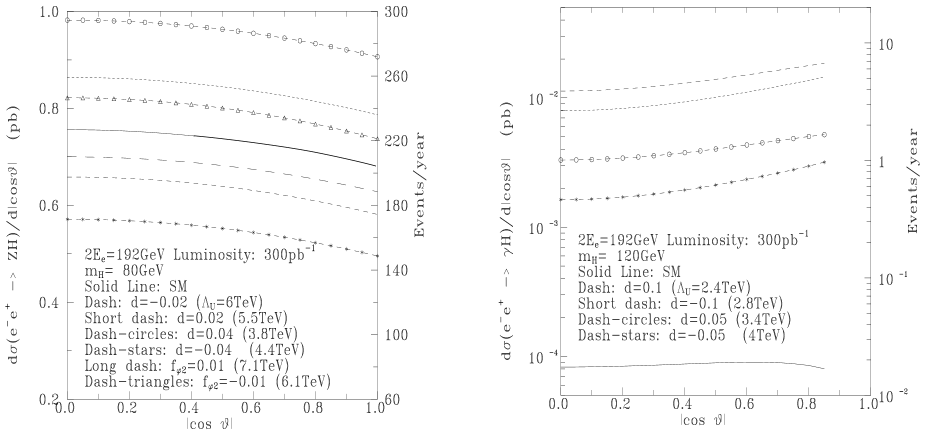
Anomalous couplings could also arise for the Higgs interactions with itself and the gauge bosons. In fact, dynamical considerations indicate that it is easier to generate anomalous couplings for the Higgs rather than for the gauge bosons [12, 13]. The dimension 6, $SU(2)\times U(1)$ invariant, CP conserving interaction is $${\cal L}_{NP}=\frac{1}{v^{2}}\,(\Phi^{\dagger}\Phi-\frac{v^{2}}{2})(d~{}\vec{\hat{W}}^{\mu\nu}\cdot\vec{\hat{W}}_{\mu\nu}+d_{B}~{}B^{\mu\nu}\ B_{\mu\nu})+\frac{4f_{\Phi 2}}{v^{2}}~{}\partial_{\mu}(\Phi^{\dagger}\Phi)\partial^{\mu}(\Phi^{\dagger}\Phi)\ .\$$ (30) The first two of the above terms generate Higgs-gauge boson interactions while the last one induces anomalous Higgs interactions through a renormalization of the Higgs field. As in section 2.1.1, unitarity can be used to associate to any given value of each of these anomalous couplings the largest allowed scale $\Lambda_{U}$ where New Physics generates it. For the first two operators these relations are $\displaystyle d\simeq\frac{104.5~{}\left({\frac{M_{W}}{\Lambda_{U}}}\right)^{2}}{1+6.5\left({\frac{M_{W}}{\Lambda_{U}}}\right)}\ \mbox{ for }d>0$ , $\displaystyle d\simeq-~{}\frac{104.5~{}\left({\frac{M_{W}}{\Lambda_{U}}}\right)^{2}}{1-4\left({\frac{M_{W}}{\Lambda_{U}}}\right)}\ \mbox{ for }d<0\ ,$ (31) $\displaystyle d_{B}\simeq\frac{195.8~{}\left({\frac{M_{W}}{\Lambda_{U}}}\right)^{2}}{1+200\left({\frac{M_{W}}{\Lambda_{U}}}\right)^{2}}\ \mbox{ for }d_{B}>0$ , $\displaystyle d_{B}\simeq-~{}\frac{195.8~{}\left({\frac{M_{W}}{\Lambda_{U}}}\right)^{2}}{1+50\left({\frac{M_{W}}{\Lambda_{U}}}\right)^{2}}\mbox{ for }d_{B}<0\ .\$ (32) Thus, for $\Lambda_{U}=1$ TeV, the largest allowed values are $d\simeq 0.4$ or $-1$ and $d_{B}\simeq 0.6$ or $-1$. The above anomalous Higgs couplings may be studied at LEP2 through the processes $e^{-}e^{+}\to ZH,$ provided $m_{H}<\sqrt{s}-M_{Z}$, or via $e^{-}e^{+}\to\gamma H$ if $m_{H}<\sqrt{s}$. Considering tree level anomalous contributions and restricting to cases where only one of the operators above is active [83, 84, 85, 86], we get the results given in the figures below. Figure 14: Distribution of Higgs production angle, $d\sigma/d{\rm cos}\theta$, for (a) $HZ$ production at $m_{H}=80$ GeV and (b) $H\gamma$ production at $m_{H}=120$ GeV. Thus, from Fig. 14a, presenting $e^{-}e^{+}\to ZH$, we deduce observability limits $|f_{\phi 2}|\simeq 0.01$ and $|d|\simeq 0.015$ ($|d_{B}|\simeq 0.05$) corresponding to $\Lambda_{U}\simeq 6-7$ TeV ( $\Lambda_{U}\simeq 5$ TeV) for $m_{H}\simeq 80$ GeV. More striking is the process $e^{-}e^{+}\to\gamma H$ which is unobservable at LEP2 in the SM [87, 88], but may become observable in the presence of NP interactions for the Higgs. A sensitivity to $|d|\simeq 0.05$ or $|d_{B}|\simeq 0.025$ should be possible from this process for $m_{H}\sim 80$ GeV, which means testing NP scales up to 3 and 7 TeV, respectively[86].

11 Conclusions

Experiments at LEP2 will allow a precise direct measurement of the most immediate consequence of the non-Abelian character of the electroweak bosons, the TGC of the $W$ to the photon and the $Z$. Various channels can provide information on non-standard interactions in the bosonic sector. The process $e^{-}e^{+}\to f\bar{f}$ determines oblique parameters which are complementary to LEP1 results. $Z\gamma$, $HZ$ and $H\gamma$ production allow one to search for non-standard boson couplings in the neutral sector. $e^{-}e^{+}\to\nu\bar{\nu}\gamma$ is marginally sensitive to the $WW\gamma$ coupling in isolation. However, the most important process is clearly $e^{-}e^{+}\to W^{-}W^{+}$ or its generalization, 4 fermion production. Of the various decay channels, the semileptonic modes $W^{-}W^{+}\to jje\nu,\;jj\mu\nu$ will provide the most precise individual measurements of TGCs, since high statistics and almost complete information on the decay distributions are combined. Of particular importance is the identification of the $W$ charge which is needed to measure the full production angle distribution $d\sigma/d{\rm cos}\theta$. Also, the decay angular distributions and their correlations with each other and with the $W$ production angle are needed to resolve the correlations between different TGCs to a maximal extent. A priori, the $jjjj$ final state provides incomplete information on the $W$ charges. However, correct charge assignments at the 80% level can be obtained by determining weighted jet charges, providing potentially valuable additional information in TGC determination. While more limited in statistics, the leptonic channel, $\ell\nu\ell\nu$, is particularly clean, and the $jj\tau\nu$ channel will also be of use in TGC analyses. Using $jje\nu$ and $jj\mu\nu$ data alone, measurements of particular TGC parameters at $\sqrt{s}=192$ GeV appear possible at generator level with a precision of $\approx\pm 0.02$ for an integrated luminosity of 500 pb${}^{-1}$. The effects of ISR and finite $W$-width and the application of experimental selection, acceptance and reconstruction procedures lead to a degradation estimated at $\approx 30-40\%$ in the precision, and to a systematic shift which is a factor 3 larger than the statistical error, but our studies indicate that this bias can be corrected. For more general TGCs, considerable cancellation between different parameters is possible, resulting in weaker bounds. It is for this case that information from the full five-fold angular distribution of $W^{-}W^{+}$ production and decay angles or its generalization to 4-fermion final states becomes particularly important.