Heavy Fermions Virtual Effects at $e^{+}e^{-}$ Colliders

Stefano Rigolin

Dipartimento di Fisica, Universitá di Padova, Italy

INFN, Sezione di Padova, Padova, Italy

E-Mail Address: RIGOLIN@VAXFPD.PD.INFN.IT

We derive the low-energy electroweak effective lagrangian for the case of additional heavy, unmixed, sequential fermions. Present LEP1 data still allow for the presence of a new quark and/or lepton doublet with masses greater than $M_{Z}/2$, provided that these multiplets are sufficiently degenerate. Keeping in mind this constraint, we analyse the virtual effects of heavy chiral fermions in $e^{+}e^{-}\rightarrow W^{+}W^{-}$ process at energies $\sqrt{p^{2}}=200,~{}500,~{}1000$ GeV, provided by LEP2 and Next Linear Collider. The effects will be unobservable at LEP2, being smaller than $3.0\cdot 10^{-3}$, while more interesting is the case of NLC, where an enhancement factor, due to a delay of unitarity, gives deviations from SM of the order 10-50 per cent, for a wide range of new fermions masses.

Talk given at the XIX International School of Theoretical Physics: ”Particle Physics and Astrophysics in the Standard Models and Beyond”, Bystra, 19-26 September 1995.

1 Introduction

LEP1 precision data represent a step of paramount relevance in probing extensions of the Standard Model (SM). Through their virtual effects, the electroweak radiative corrections ”feel” the presence of new particles running in the loops and the level of accuracy on the relevant observables is such that this set of tests is complementary to the traditional probes on virtual effects due to new physics (i.e. highly suppressed or forbidden flavour changing neutral current phenomena). In some cases, as that which we aim to discuss here, the electroweak precision tests represent the only indirect way to search for these new particles.

We will discuss electroweak radiative effects from extensions of the ordinary fermionic spectrum of the SM. The new fermions are supposed to possess the same colour and electroweak quantum numbers as the ordinary ones and to mix very tinily with the ordinary three generations. The most straightforward realization of such a fermionic extension of the SM is the introduction of a fourth generation of fermions. This possibility has been almost entirely jeopardized by the LEP1 bound on the numbers of neutrinos species. Although there still exists the obvious way out of having new fermion generations with heavy neutrinos, we think that these options are awkward enough not to deserve further studies. Rather, what we have in mind in tackling this problem are general frames discussing new physics beyond the SM which lead to new quarks and/or leptons classified in the usual chiral way with iso-doublets and iso-singolets for different chiralities. Situations of this kind may be encountered in grand unified schemes where the ordinary fifteen Weyl spinors of each fermionic generation are only part of larger representations or where new fermions (possibly also mirror fermions) are requested by the group or manifold structure of the schemes. Chiral fermions with heavy static masses may also provide a first approximation of virtual effects in techicolor-like schemes when the dynamical behaviour of technifermion self-energies are neglected.

Although such effects have been extensively investigated in the literature [1], our presentation focuses mainly on two aspects, which have been only partially touched in the previous analyses: the use of effective lagrangians for a model-independent treatment of the problem and a discussion of the validity of this approach in comparison with the computation in the full-fledged theory.

While separate tests can be set up for each different extension of the SM, there may be some advantage in realizing this analysis in a model independent framework. The natural theoretical tool to this purpose is represented by an effective electroweak lagrangian where, giving up the renormalizability requirement, all $SU(2)_{L}\otimes U(1)_{Y}$ invariant operators up to a given dimension are present with unknown coefficients, to be eventually determined from the experiments. Each different model fixes uniquely this set of coefficients and the effective lagrangian becomes in this way a common ground to discuss and compare several SM extensions. The introduction of the well known $S$, $T$ and $U$ [2] or $\epsilon$’s [3] variables was much in the same spirit and the use of an effective lagrangian represents in a sense the natural extension of these approaches (section 2).

We derive (section 3) some constrains on new chiral doublets, from latest avaible values of the $\epsilon$’s data, in the effective lagrangians approximation and in the full one-loop computation, putting on evidence that deviations are sizeable (compared with experimental errors) only for fermion masses close to the $M_{Z}/2$ threshold. Some of the constraints on new sequential fermions coming from $p\bar{p}$ accelerator results are also presented.

But LEP1 analysis is not important only for studying the existence of new physics in the bilinear sector. Also trilinear coupling are severely constrained by the presence of observed bilinear effects at LEP1-SLC. To avoid ambiguities in the forms factor definitions at one loop level, we present an analysis of new chiral fermions effects on $e^{+}e^{-}\rightarrow W^{+}W^{-}$ differential cross-section. Here it will be evident that the delay’s of unitarity effects makes higher energies collider ($\sqrt{p^{2}}=500$ GeV, or $1000$ GeV, much more sensitive than LEP2 to this kind of new physics effects (section 4).

2 Effective Lagrangian Approach

The use of an effective lagrangian for the electroweak physics has been originally advocated for the study of the large Higgs mass limit in the SM [4, 5, 6]. Subsequently, contributions from chiral $SU(2)_{L}$ doublets have been considered in the degenerate case [7], for small splitting [9] and in the case of infinite splitting [10, 13]. In the present note we will deal with the general case of arbitrary splitting among the fermions in the doublet [11].

Here, for completeness, we consider the standard list of $SU(2)_{L}\otimes U(1)_{Y}$ CP conserving operators containing up to four derivatives and built out of the gauge vector bosons $W^{i}_{\mu}~{}~{}(i=1,2,3),~{}B_{\mu}$ and the would be Goldstone bosons $\xi^{i}$ [5]:

$${\cal L}_{0} = \displaystyle\frac{v^{2}}{4}[tr(TV_{\mu})]^{2}$$

$${\cal L}_{1} = i\displaystyle\frac{gg^{\prime}}{2}B_{\mu\nu}tr(T\hat{W}^{\mu\nu})$$

$${\cal L}_{2} = i\displaystyle\frac{g^{\prime}}{2}B_{\mu\nu}tr(T[V^{\mu},V^{\nu}])$$

$${\cal L}_{3} = g~{}tr(\hat{W}_{\mu\nu}[V^{\mu},V^{\nu}])$$

$${\cal L}_{4} = [tr(V_{\mu}V_{\nu})]^{2}$$

$${\cal L}_{5} = [tr(V_{\mu}V^{\mu})]^{2}$$

$${\cal L}_{6} = tr(V_{\mu}V_{\nu})tr(TV^{\mu})tr(TV^{\nu})$$

$${\cal L}_{7} = tr(V_{\mu}V^{\mu})[tr(TV^{\nu})]^{2}$$

$${\cal L}_{8} = \displaystyle\frac{g^{2}}{4}[tr(T\hat{W}_{\mu\nu})]^{2}$$

$${\cal L}_{9} = \displaystyle\frac{g}{2}tr(T\hat{W}_{\mu\nu})tr(T[V^{\mu},V^{\nu}])$$

$${\cal L}_{10} = [tr(TV_{\mu})tr(TV_{\nu})]^{2}$$

$${\cal L}_{11} = tr(({\cal D}_{\mu}V^{\mu})^{2})$$

$${\cal L}_{12} = tr(T{\cal D}_{\mu}{\cal D}_{\nu}V^{\nu})tr(TV^{\mu})$$

$${\cal L}_{13} = \displaystyle\frac{1}{2}[tr(T{\cal D}_{\mu}V_{\nu})]^{2}$$

$${\cal L}_{14} = i~{}g~{}\epsilon^{\mu\nu\rho\sigma}~{}tr(\hat{W}_{\mu\nu}V_{\rho})tr(TV_{\sigma})$$ (1)

We recall the notation used. If we define the Goldstone boson contribution $U=exp(i\vec{\xi}\cdot\vec{\tau}/v)$ (so that in the unitary gauge $U=1$), than:

$$T=U\tau^{3}U^{\dagger}~{}~{}~{},~{}~{}~{}V_{\mu}=(D_{\mu}U)U^{\dagger}~{}~{}~{},$$ (2)

$$D_{\mu}U=\partial_{\mu}U-g\hat{W}_{\mu}U+g^{\prime}U\hat{B}_{\mu}~{}~{}~{},$$ (3)

where $\hat{W}_{\mu},~{}\hat{B}_{\mu}$ are the matrices collecting the gauge fields:

$$\hat{W}_{\mu}=\frac{1}{2i}\vec{W}_{\mu}\cdot\vec{\tau}~{}~{}~{},~{}~{}~{}\hat{B}_{\mu}=\frac{1}{2i}B_{\mu}\tau^{3}~{}~{}~{}.$$ (4)

The corresponding field strengths are given by:

$$\hat{W}_{\mu\nu} = \partial_{\mu}\hat{W}_{\nu}-\partial_{\nu}\hat{W}_{\mu}-g[\hat{W}_{\mu},\hat{W}_{\nu}]{}~{}~{}~{},$$

$$\hat{B}_{\mu\nu} = \partial_{\mu}\hat{B}_{\nu}-\partial_{\nu}\hat{B}_{\mu}~{}~{}~{}.$$ (5)

Finally the covariant derivative acting on $V_{\mu}$ is given by:

$${\cal D}_{\mu}V_{\nu}=\partial_{\mu}V_{\nu}-g[\hat{W}_{\mu},V_{\nu}]~{}~{}~{}.$$ (6)

The effective electroweak lagrangian reads:

$${\cal L}_{eff}={\cal L}_{SM}+\sum_{i=0}^{14}a_{i}{\cal L}_{i}~{}~{}~{},$$ (7)

where ${\cal L}_{SM}$ is the ”low-energy” SM lagrangian, and all the contributions of the new physics heavy sectors is contained in the $a_{i}$ coefficients .

We have determined the coefficients $a_{i}~{}(i=0,...,14)$, for an extra doublet of heavy fermions (quarks or leptons), by computing the corresponding one-loop contribution to a set of $n$-point gauge boson functions $(n=2,3,4)$, in the limit of low external momenta. For example just look at the two-point vector boson functions $-i\Pi^{\mu\nu}_{ij}(p)$. In the limit $p^{2}\ll 4M^{2}$, we can use a derivative expansion around $p^{2}=0$:

$$\Pi^{\mu\nu}_{ij}(p) = g^{\mu\nu}\Pi_{ij}(p^{2})+(p^{\mu}p^{\nu}~{}~{}{\rm terms})~{}~{}~{}~{}~{}~{}~{}~{}~{}~{}~{}~{}~{}~{}~{}~{}~{}~{}~{}~{}~{}~{}~{}(i,j=0,1,2,3)$$

$$\Pi_{ij}(p^{2}) \equiv A_{ij}+p^{2}F_{ij}(p^{2})=A_{ij}+p^{2}F_{ij}(0)+...$$ (8)

The next terms in the $p^{2}$ expansion are suppressed by increasing powers of $p^{2}/M^{2}$, ($M$ generically representing the mass of the particles running in the loop), and so will be neglected in this effective lagrangian approach. By denoting with $M$ and $m$ the masses of the upper and lower weak isospin components and with $r=m^{2}/M^{2}$ the square ratio, we obtain, in units of $1/16\pi^{2}$:

$$a^{q}_{0} = {3M^{2}\over 2v^{2}}\left({1-r^{2}+2\,r\,\log r\over 1-r}\right)$$

$$a^{q}_{1} = \frac{1}{12(-1+r)^{3}}\left[{3(1-15r+15r^{2}-r^{3})+2(1-12r-6r^{2}-r^{3})\log r}\right]$$

$$a^{q}_{2} = \frac{1}{12(-1+r)^{3}}\left[{3(3-7\,r+5\,{r^{2}}-r^{3})+2\,(1-{r^{3}})\,\log r}\right]$$

$$a^{q}_{3} = \frac{1}{8(-1+r)^{3}}\left[3(-1+7\,r-7\,{r^{2}}+{r^{3}})+6\,r\,(1+{r})\,\log r)\right]$$

$$a^{q}_{4} = \frac{1}{6(-1+r)^{3}}\left[5-9\,r+9\,{r^{2}}-5\,{r^{3}}+3\,(1+{r^{3}})\,\log r\right]$$

$$a^{q}_{5} = \frac{1}{24(-1+r)^{3}}\left[-23+45\,r-45\,{r^{2}}+23\,{r^{3}}-12\,(1+{r^{3}})\,\log r\right]$$

$$a^{q}_{6} = \frac{1}{24(-1+r)^{3}}\left[-23+81\,r-81\,r^{2}+23\,r^{3}-6\,(2-3\,r\,-3\,r^{2}\,+2\,r^{3})\,\log r\right]$$

$$a^{q}_{7} = -a^{q}_{6}$$

$$a^{q}_{8} = \frac{1}{12(-1+r)^{3}}\left[7-81\,r+81\,r^{2}-7\,r^{3}+6\,(1-6\,r\,-6\,r^{2}\,+r^{3})\,\log r\right]$$

$$a^{q}_{9} = -a^{q}_{6}$$

$$a^{q}_{10} = 0$$

$$a^{q}_{11} = -{1\over{2}}$$

$$a^{q}_{12} = \frac{1}{8(-1+r)^{3}}\left[1+9\,r-9\,{r^{2}}-{r^{3}}+6\,r\,(1+{r})\,\log r\right]$$

$$a^{q}_{13} = 2\,a^{q}_{12}$$

$$a^{q}_{14} = \frac{3}{8(-1+r)^{2}}\left[1-r^{2}+2r\log r\right]$$ (9)

for quarks, and:

$$a^{l}_{i} = \frac{1}{3}a^{q}_{i}~{}~{}~{}~{}~{}~{}~{}~{}~{}(i=0,~{}~{}i=3,...14)$$

$$a^{l}_{1} = \frac{1}{12(-1+r)^{3}}\left[1-15r+15r^{2}-r^{3}-2\,(1+6r^{2}-r^{3})\log r\right]$$

$$a^{l}_{2} = \frac{1}{12(-1+r)^{3}}\left[-1-3\,r+9r^{2}-5r^{3}-2\,(1-r^{3})\,\log r\right]$$ (10)

for leptons.

Indeed the use of an effective lagrangian in precision tests has its own limitations. One can ask how large has to be $M$ to obtain a sensible approximation from the truncation of the full one-loop result. We will see this aspects in the next section.

3 Two Point Functions

For new chiral fermions which do not mix with the ordinary ones, the virtual effects measurable at LEP1 are all described by operators bilinear in the gauge vector bosons. We will describe these effects in the approximate effective theory (we can call it with evident meaning ”static approximation”), as well in the full one-loop calculation.

3.1 Static Approximation

The coefficients $a_{i}$ of the effective lagrangian ${\cal L}_{eff}$ are related to measurable parameters. In particular, to make contact with the LEP1 data, we recall that, by neglecting higher derivatives, the relation between the effective lagrangian ${\cal L}_{eff}$ and the $\epsilon_{i}$ parameters, is given by:

$$\Delta\epsilon_{1} = 2a_{0}~{},$$

$$\Delta\epsilon_{2} = -g^{2}(a_{8}+a_{13})~{},$$

$$\Delta\epsilon_{3} = -g^{2}(a_{1}+a_{13})~{}.$$ (11)

where $\Delta\epsilon_{i}$ are the new physics contributions to the $\epsilon$’s. From eqs. (9) and (10) one finds:

$$\Delta\epsilon^{q}_{1}=3\Delta\epsilon^{l}_{1}={3M^{2}\over 8\pi^{2}}{G\over\sqrt{2}}\left[{1-r^{2}+2\,r\,\log r\over(1-r)}\right]$$ (12)

$$\Delta\epsilon^{l}_{2}=3\Delta\epsilon^{l}_{2}={Gm_{W}^{2}\over 12\pi^{2}\sqrt{2}}\left[{5-27r+27r^{2}-5r^{3}+\left(3-9r-9r^{2}+3r^{3}\right)\log r\over\left(1-r\right)^{3}}\right]$$ (13)

$$\Delta\epsilon^{q}_{3}={Gm_{W}^{2}\over 12\pi^{2}\sqrt{2}}\left[3+\log r\right]$$ (14)

$$\Delta\epsilon^{l}_{3}={Gm_{W}^{2}\over 12\pi^{2}\sqrt{2}}\left[1-\log r\right]$$ (15)

The $\epsilon_{i}$ parameters are obtained by adding to $\Delta\epsilon_{i}$ the SM contribution $\epsilon^{SM}_{i}$, which we regard as functions of the Higgs and top quark masses. A recent analysis of the available precision data from LEP1, SLD, low-energy neutrino scatterings and atomic parity violation experiments, leads to the following values for the $\epsilon_{i}$ parameters [14]:

$$\epsilon_{1} = (3.6\pm 1.5)\cdot 10^{-3}$$

$$\epsilon_{2} = (-5.8\pm 4.3)\cdot 10^{-3}$$

$$\epsilon_{3} = (3.6\pm 1.5)\cdot 10^{-3}$$ (16)

Notice the relatively large error in the determination of $\epsilon_{2}$, mainly dominated by the uncertainty on the $W$ mass.

It is clear from eq. (9) and from eqs. (11–15) that only $\Delta\epsilon_{1}$ can have a huge contribution proportional to $M^{2}$. But, as it is well known, this term is vanishing in the limit of degenerate doublet. From the analysis of this parameter we can obtain only a limitation of the splitting of the fermion masses, and not an ”absolute” statement on the number of possible extra doublets. In fig.1 we can see that if for relatively light masses $M=200$ GeV (dotted line) a small splitting is still allowed, ($0.5\leq r\leq 1.5$), for heavier masses, like for example $M=1000$ GeV (full line), the doublet must be practically degenerate ($0.91\leq r\leq 1.08$).

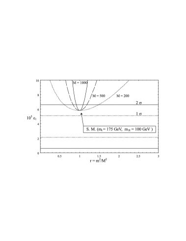
Figure 1: Predictions for $\epsilon_{1}$ from an additional heavy quark doublet with masses $M=200$ GeV (dotted line), $M=500$ GeV (dashed line), $M=1000$ GeV (full line), for $m_{t}=175$ GeV and $M_{H}=100$ GeV. The $1\sigma$ (dotted horizontal line) and $2\sigma$ (full horizontal line) allowed region are also displayed. The values $\epsilon_{1}(r=1)$ is the SM predictions for the fixed $m_{t}=175$ GeV and $M_{H}=100$ GeV.

The contributions from $\Delta\epsilon_{2}$ and $\Delta\epsilon_{3}$, have only dependence from $\log r$ and powers of $r$. Again $\Delta\epsilon_{2}$ is vanishing for $r=1$, so doesn’t give us any useful indications. Different is the case of $\Delta\epsilon_{3}$, the only bilinear parameter non null in the $r\rightarrow 1$ limit. From eq. (15) we have:

$$\Delta\epsilon^{q}_{3}=3\Delta\epsilon^{l}_{3}={Gm_{W}^{2}\over 4\pi^{2}\sqrt{2}}\simeq 1.3\cdot 10^{-3}$$ (17)

Thus, with the conditions provided us by the analysis of both $\epsilon_{1}$ and $\epsilon_{3}$, we obtain an ”absolute” bound on the number of possible extra heavy fermions. The full horizontal lines in fig.2 are the $2\sigma$ deviation from the experimental value of $\epsilon_{3}$. It can be noted that at least one quark doublet (full line) is not completely ruled out by the experiment.

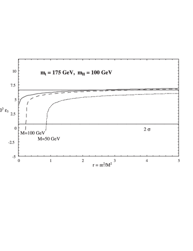
Figure 2: Comparison between the asymptotic (solid line) and full one-loop (respectively with mass $M=100$ GeV (dashed lines) and $M=50$ GeV (dotted lines)) computations of $\epsilon_{3}$ versus $r=m^{2}/M^{2}$, for an additional quark doublet. For the SM contribution, $m_{t}=175$ GeV and $m_{H}=100$ GeV are assumed. The $2\sigma$ allowed region is also displayed.

3.2 Full Calculation

We are thus lead to consider the possibility of relatively light (but obviously under production threshold), chiral fermions, both to check the agreement with the present data, and to test the reliability of our effective lagrangian approach. If the additional fermions are not sufficiently heavy, we do not expect that their one-loop effects are accurately reproduced by the coefficients $a_{i}$ in eqs. (9-10). In this case we have to consider the full dependence on external momenta of the Green functions, not just the first two terms of the $p^{2}$ expansion given in eq. (8). We recall that in this case the $\epsilon$ parameters are given by [15]:

$$\Delta\epsilon_{1} = e_{1}-e_{5}(m_{Z}^{2})$$

$$\Delta\epsilon_{2} = e_{2}-s^{2}~{}e_{4}-c^{2}~{}e_{5}(m_{Z}^{2})$$

$$\Delta\epsilon_{3} = e_{3}(m_{Z}^{2})+c^{2}~{}e_{4}-c^{2}~{}e_{5}(m_{Z}^{2})$$ (18)

where we have kept into account the fact that in our case there are no vertex or box corrections to four-fermion processes. In eq. (18)

$$e_{1} = \frac{\Pi_{ZZ}(0)}{m_{Z}^{2}}-\frac{\Pi_{WW}(0)}{m_{W}^{2}}$$

$$e_{2} = \Pi^{\prime}_{WW}(0)-c^{2}~{}\Pi^{\prime}_{ZZ}(0)-2sc~{}\frac{\Pi_{\gamma Z}(m_{Z}^{2})}{m_{Z}^{2}}-s^{2}~{}\Pi^{\prime}_{\gamma\gamma}(m_{Z}^{2})$$

$$e_{3}(p^{2}) = \frac{c}{s}\left\{sc\left[\Pi^{\prime}_{\gamma\gamma}(m_{Z}^{2})-\Pi^{\prime}_{ZZ}(0)\right]+(c^{2}-s^{2})~{}\frac{\Pi_{\gamma Z}(p^{2})}{p^{2}}\right\}$$

$$e_{4} = \Pi^{\prime}_{\gamma\gamma}(0)-\Pi^{\prime}_{\gamma\gamma}(m_{Z}^{2})$$

$$e_{5}(p^{2}) = \Pi^{\prime}_{ZZ}(p^{2})-\Pi^{\prime}_{ZZ}(0)$$ (19)

We introduce also (for later use) $\Delta\alpha(p^{2})$, $\Delta k(p^{2})$, $\Delta\rho(p^{2})$, $\Delta r_{W}$ and $e_{6}$ by the following relations in terms of the unrenormalized vector-boson vacuum polarizations:

$$\Delta\alpha(p^{2}) = \Pi^{\prime}_{\gamma\gamma}(0)-\Pi^{\prime}_{\gamma\gamma}(p^{2})$$

$$\Delta k(p^{2}) = -\frac{c^{2}}{c^{2}-s^{2}}~{}(e_{1}-e_{4})+\frac{1}{c^{2}-s^{2}}~{}e_{3}(p^{2})$$

$$\Delta\rho(p^{2}) = e_{1}-e_{5}(p^{2})$$

$$\Delta r_{W} = -\frac{c^{2}}{s^{2}}~{}e_{1}+\frac{c^{2}-s^{2}}{s^{2}}~{}e_{2}+2~{}e_{3}(m^{2}_{Z})+e_{4}$$

$$e_{6} = \Pi^{\prime}_{WW}(m_{W}^{2})-\Pi^{\prime}_{WW}(0)$$ (20)

where we have:

$$\Pi^{\prime}_{VV}(p^{2})=\frac{\Pi_{VV}(p^{2})-\Pi_{VV}(m_{V}^{2})}{(p^{2}-m_{V}^{2})}~{}~{}~{},~{}~{}~{}~{}~{}~{}~{}~{}~{}~{}~{}~{}~{}~{}~{}~{}~{}~{}~{}~{}~{}~{}~{}~{}~{}~{}~{}~{}~{}V=(\gamma,Z,W)$$ (21)

and finally, the effective sine is defined:

$$s^{2}=\frac{1}{2}-\sqrt{\frac{1}{4}-\frac{\pi\alpha(m^{2}_{Z})}{\sqrt{2}G_{F}m_{Z}^{2}}}$$ (22)

If $p^{2}=m_{Z}^{2}$ then $\Delta\alpha(p^{2})$, $\Delta k(p^{2})$, $\Delta\rho(p^{2})$, $\Delta r_{W}$ coincides with the corrections $\Delta\alpha$, $\Delta k$, $\Delta\rho$ and $\Delta r_{W}$ which characterize the electroweak observables at the $Z$ resonance . The expressions for the quantities $e_{i}$, in the case of an ordinary quark or lepton doublet can be easily derived from the literature [16].

In fig.3 we illustrate our full one loop result in the plane $(\epsilon_{1},\epsilon_{3})$, for the case of an extra quark doublet. The upper ellipsis represents the $1\sigma$ experimentally allowed region, obtained by combining all LEP1 data. We plot the result for an extra quark doublet (full line) taking $m_{t}=175$ GeV and $m_{H}=100$ GeV. One of the two masses is kept fixed at $50$ GeV, and the other one runs from $50$ GeV to $170$ GeV. One has in this way two branches, according to which mass, $m$ or $M$, has been fixed. If at least one of the two masses is small, this causes a substantial deviation from the asymptotic, effective lagrangian prediction. In particular, as it was observed in [15], a large negative contribution to both $\epsilon_{1}$ and $\epsilon_{3}$ is now possible, due to a formal divergence of $\Pi^{\prime}_{ZZ}(m_{Z}^{2})-\Pi^{\prime}_{ZZ}(0)$ at the threshold which produces a large and positive $e_{5}$. Clearly, this behaviour cannot be reproduced by ${\cal L}_{eff}$, which, at the fourth order in derivatives, automatically sets $e_{5}=0$. The dashed line shows the predictions when all the two masses of the additional quark doublet are heavy. Here we fix one of the masses to $200$ GeV and let the other vary from $200$ GeV to $300$ GeV. As before the top and Higgs masses has been fixed to $175$ GeV and $100$ GeV. As expected, it appears that only a small amount of splitting among the doublet components is allowed. For the chosen value of $m_{t}$ and $m_{H}$, the SM prediction lies already outside the $1\sigma$ allowed region and additional positive contributions to $\epsilon_{1}$ tend to be disfavoured. On the contrary, the positive contribution to $\epsilon_{3}$, almost constant in the chosen range of masses, is still tolerated. If one also includes the SLD determination of the left-right asymmetry, then one gets the lower ellipsis.

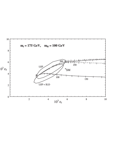
Figure 3: Predictions for $\epsilon_{1}$, $\epsilon_{3}$ from an additional quark doublet. The lower (upper) dashed line represents the case $m~{}(M)~{}=200$ GeV, $M~{}(m)$ varying between $200$ GeV and $300$ GeV, evaluated with ${{\cal L}}_{eff}$. The lower (upper) full line corresponds to $m~{}(M)~{}=50$ GeV, $M~{}(m)$ varying between $50$ GeV and $170$ GeV, evaluated with a complete 1-loop computation. The SM point corresponds to $m_{t}=175$ GeV and $m_{H}=100$ GeV. The upper (lower) ellipses is the $1\sigma$ allowed region, obtained by a fit of the high energy data which excludes (includes) the SLD measurement.

A relevant question is, then, when the asymptotical regime starts, i.e. how close to $M_{Z}$ should be the masses of the new quarks or leptons for observing deviations due to the full expression of $\Pi_{ij}(p^{2})$ instead of the truncated expression given in eq. (8). A detailed analysis shows that already for masses of the new fermions above $70-80$ GeV the difference between the values of the $\epsilon_{i}$ obtained with the truncated and full expression of $\Pi_{ij}(p^{2})$ are as small as $10^{-4}$, i.e. below the present experimental level of accuracy. This is illustrated in fig.2 where the asymptotical (full line) and full one loop (dashed and dotted) expression of $\epsilon_{3}$ are compared as a function of $r$.

Beyond the indirect precision tests, the possibility of having new fermions carrying the usual $SU(3)_{C}\times SU(2)_{L}\times U(1)_{Y}$ quantum numbers can clearly also be bounded by the direct searches. Concerning the present searches, from LEP1 we have the lower bound of $M_{Z}/2$ which applies independently from any assumption on the decay modes of the new fermions which couple to the $Z$ boson. Much stronger limits on the new quark masses can be inferred from the Tevatron results. However, as we know from the search for the top quark, these latter bounds rely on assumptions concerning the decay modes of the heavy quark. For instance, in the case of the top search it was stressed that if a new decay channel into the $b$ quark and a charged Higgs were avaible to the top, then one could not use the CDF bounds on $m_{t}$ [17] which came along these last years, before the final discovery of the top quark.

Now, it may be conceivable that the new physics related to the presence of extra-fermions can also affect their possible decay channels making the lightest of the new fermions unstable. Indeed, we stated in our assumption that the new fermions do not essentially mix with the ordinary ones, hence one has to invoke new physics if one wants to avoid the formation of stable heavy mesons made out of the lightest stable new fermion and of the ordinary fermions of the Standard Model. If the new fermions can decay within the detector, then the bounds on their masses, coming from Tevatron data, must be discussed in a model-dependent way and even the case of new quarks with masses lighter than $m_{t}$ are not fully ruled out.

If on the contrary the lightest new quark is stable, then searches for exotic heavy meson at CDF already ruled out the possibility of being near the threshold $M_{Z}/2$. The existence of coloured particle with charge $\pm 1$ is strictly bounded over $130\ GeV$ from CDF experiment [19]. Finally, note that for charged leptons the bound coming from CDF are much less stringent. A new stable charged lepton of mass of $60-70\ GeV$ cannot be ruled out.

4 Three Points Functions

If new physics beyond the SM were modeled by additional heavy chiral fermions, of the kind we have considered, then we could draw informations on the searches, at future colliders, of anomalous trilinear gauge boson couplings of the $WWV$ vertex (where $V$ stands for neutral vector boson). We define the kinematics of the $WWV$ vertex as

$$V(p,v_{1})\rightarrow W^{-}(q,v_{2})+W^{+}(\bar{q},v_{3})~{}~{}~{}~{}~{},$$ (23)

where $p,q,\bar{q}$ are the momenta of $V,W^{-},W^{+}$ respectively, and $v_{1},v_{2},v_{3}$ are their polarization vectors. For simplicity we can impose the produced $W^{\pm}$ to be on shell, so:

$$q^{2}=\bar{q}^{2}=m_{W}^{2}~{}~{}~{}~{},~{}~{}~{}~{}q\cdot v_{2}=\bar{q}\cdot v_{3}=0~{}~{}~{}~{}~{}.$$ (24)

Following the definitions of [23], the general CP-conserving coupling of two on-shell charged vector bosons with a neutral vector boson ($V=\gamma,Z$) can be derived from the following effective lagrangians:

$$\frac{{\cal L}_{WWV}}{g_{WWV}} = ig_{1}^{V}(W_{\mu\nu}^{\dagger}W^{\mu}V^{\nu}-W_{\mu}^{\dagger}V^{\nu}W_{\mu\nu})+i\kappa_{V}W_{\mu}^{\dagger}W^{\nu}V^{\nu\mu}$$ (25)

$$+ i\frac{\lambda_{V}}{\Lambda^{2}}W_{\lambda\mu}^{\dagger}W^{\mu}_{\nu}V^{\nu\lambda}+g_{5}^{V}\epsilon^{\mu\nu\rho\sigma}(W_{\mu}^{\dagger}\stackrel{{\scriptstyle\leftrightarrow}}{{\partial}}_{\rho}W_{\nu})V_{\sigma}~{}~{}~{}~{},$$

where $V_{\mu}$ is the neutral vector boson field, $W_{\mu}$ is the field associated with the $W^{-}$, $W_{\mu\nu}=\partial_{\mu}W_{\nu}-\partial_{\nu}W_{\mu}$, $V_{\mu\nu}=\partial_{\mu}V_{\nu}-\partial_{\nu}V_{\mu}$ and $\Lambda$ is a mass scale parameter opportunely chosen. By convention $g_{WW\gamma}=-e$ and $g_{WWZ}=-e~{}c/s$.

In momentum space the $WWV$ vertex can be decomposed as

$$\Gamma_{V}^{\alpha\beta\mu}(q,\bar{q},p) = f_{1}^{V}(q-\bar{q})^{\mu}g^{\alpha\beta}-\frac{f_{2}^{V}}{m_{w}^{2}}(q-\bar{q})^{\mu}p^{\alpha}p^{\beta}+f_{3}^{V}(p^{\alpha}g^{\mu\nu}-p^{\beta}g^{\alpha\mu})$$ (26)

$$+ if_{5}^{V}\epsilon^{\alpha\beta\mu\sigma}(q-\bar{q})_{\sigma}.$$

Here all the forms factors $f_{i}^{V}$ are dimensionless functions of $p^{2}$. From eqs. (25-26) it is easy to recover the following relations:

$$f_{1}^{V} = g_{1}^{V}+\frac{p^{2}}{2\Lambda^{2}}\lambda_{V}$$

$$f_{2}^{V} = \lambda_{V}$$

$$f_{3}^{V} = g_{1}^{V}+\kappa_{V}+\lambda_{V}$$

$$f_{5}^{V} = g_{5}^{V}$$ (27)

Obviously we can add to these effective lagrangians ${\cal L}_{WWV}$ higher dimension operators, by replacing $V_{\mu}$ by $\partial^{2n}V_{\mu}$ (with n arbitrary integer). Higher order operators in eq. (25) will contribute with $p^{2n}$ terms to the right side of eq. (27). We need only the 4 form factors of eq. (26) for parametrizing all the new physics effects in the trilinear gauge effects.

If we are working a tree level all is univocally defined. But if we are adding also one loop contributions, one has to declare exactly which contributions wants to include in the ”form factors” definitions. Defining a renormalization depending quantity ${\cal K}$ we can write the forms factors as:

$$f^{V}_{i}=f^{SM}_{i}+\Delta f^{V}_{i}~{}~{}~{}~{}~{}~{},~{}~{}~{}~{}~{}~{}\Delta f^{V}_{i}={\cal K}\,f^{SM}_{i}+\delta f^{V}_{i}~{}~{}~{}~{}~{}~{}(i=1,2,3,5).$$ (28)

where $\Delta f^{V}_{i}$ denote the full one loop contributions due to new physics virtual effects, and $\delta f^{V}_{i}$ is the pure trilinear contributions. The term ${\cal K}\,f^{SM}_{i}$ depends on the choice of the overall normalization of the trilinear vertex $WWV~{}~{}(V=\gamma,Z)$, usually denoted by $g_{WWV}$, and on the renormalization scheme adopted. To avoid this indetermination we prefer to define these couplings by observing the physical process of $W^{\pm}$ pair production in $e^{+}e^{-}$ collision,

$$e^{-}(k,\sigma)~{}~{}+~{}~{}e^{+}(\bar{k},\bar{\sigma})~{}~{}\rightarrow~{}~{}W^{-}(q,\lambda)~{}~{}+~{}~{}W^{+}(\bar{q},\bar{\lambda})$$ (29)

Following [23] the helicity amplitude for this process can be written

$${\cal M}=\sqrt{2}~{}e^{2}~{}\mbox{$\tilde{\cal M}$}(\Theta)~{}\epsilon~{}d^{J_{0}}_{\Delta\sigma,\Delta\lambda}(\Theta)$$ (30)

where $\epsilon=(-1)^{\lambda}\Delta\sigma$ is a sign factor, $\Delta\sigma=\sigma-{\bar{\sigma}}$, $\Delta\lambda=\lambda-{\bar{\lambda}}$, $J_{0}=max(|\Delta\sigma|,|\Delta\lambda|)$, $\Theta$ is the scattering angle of $W^{-}$ with respect to $e^{-}$ in the $e^{+}e^{-}$ c.m. frame and $d^{J_{0}}_{\Delta\sigma,\Delta\lambda}$ are angular functions depending from the helicity of the initial and final states.

After the inclusion of the 1-loop corrections due to the heavy fermions and of the appropriate counterterms, the reduced amplitude for the process at hand reads

$$\bullet\Delta\lambda=\pm 2$$

$$\tilde{\cal M} = -\frac{\sqrt{2}}{s^{2}}\frac{\delta_{\Delta\sigma,-1}}{1+\beta^{2}-2\beta\cos\Theta}\left[1-\frac{s^{2}}{c^{2}-s^{2}}\Delta r_{W}-e_{6}\right]$$ (31)

$$\bullet|\Delta\lambda|\leq 1$$

$${\tilde{\cal M}}^{\gamma} = -\beta\delta_{|\Delta\sigma|,1}\left[1+\Delta\alpha(p^{2})\right]~{}\left[\mbox{$A_{\lambda{\bar{\lambda}}}^{SM}$}+\mbox{$\Delta A_{\lambda{\bar{\lambda}}}^{\gamma}$}\right]$$

$${\tilde{\cal M}}^{Z} = \beta~{}\frac{p^{2}}{p^{2}-m_{Z}^{2}}~{}\left[\delta_{|\Delta\sigma|,1}-\frac{\delta_{\Delta\sigma,-1}}{2s^{2}(1+\Delta k(p^{2}))}\right]$$

$$~{}~{}~{}~{}~{}~{}~{}~{}~{}~{}~{}~{}~{}~{}~{}~{}~{}~{}~{}~{}~{}~{}~{}\left[1+\Delta\rho(p^{2})+\frac{c^{2}-s^{2}}{c^{2}}\Delta k(p^{2})\right]~{}\left[\mbox{$A_{\lambda{\bar{\lambda}}}^{SM}$}+\mbox{$\Delta A_{\lambda{\bar{\lambda}}}^{Z}$}\right]$$

$${\tilde{\cal M}}^{\nu} = \frac{\delta_{\Delta\sigma,-1}}{2s^{2}~{}\beta}\left[1-\frac{s^{2}}{c^{2}-s^{2}}\Delta r_{W}-e_{6}\right]\left[B^{SM}_{\lambda{\bar{\lambda}}}-\frac{1}{1+\beta^{2}-2\beta\cos\Theta}C^{SM}_{\lambda{\bar{\lambda}}}\right]$$ (32)

with $\beta=(1-4m_{W}^{2}/p^{2})^{1/2}$. $A_{\lambda{\bar{\lambda}}}^{SM}$, $B^{SM}_{\lambda{\bar{\lambda}}}$ and $C^{SM}_{\lambda{\bar{\lambda}}}$ are the tree-level SM coefficients listed in Tab.1.

$\lambda\bar{\lambda}$	$A_{\lambda{\bar{\lambda}}}^{SM}$	$B^{SM}_{\lambda\bar{\lambda}}$	$C^{SM}_{\lambda\bar{\lambda}}$
$++\,,\,--$	$1$	1	$1/\gamma^{2}$
$+0\,,\,0-$	$2\gamma$	$2\gamma$	$2(1+\beta)/\gamma$
$0+\,,\,-0$	$2\gamma$	$2\gamma$	$2(1-\beta)/\gamma$
$00$	$2\gamma^{2}+1$	$2\gamma^{2}$	${2/\gamma^{2}}$

Table 1: Standard Model coefficients expressed in terms of $\gamma^{2}=p^{2}/4m_{W}^{2}$.

The coefficients $\Delta A_{\lambda{\bar{\lambda}}}^{\gamma}$ and $\Delta A_{\lambda{\bar{\lambda}}}^{Z}$ can be expressed in terms of the $CP$-invariant form factors according to the relations:

$$\Delta A_{++}^{V} = \Delta A_{--}^{V}=\Delta f_{1}^{V}$$

$$\Delta A_{+0}^{V} = \Delta A_{0-}^{V}=\gamma(\Delta f_{3}^{V}-i\Delta f_{5}^{V})$$

$$\Delta A_{-0}^{V} = \Delta A_{0+}^{V}=\gamma(\Delta f_{3}^{V}+i\Delta f_{5}^{V})$$

$$\Delta A_{00}^{V} = \gamma^{2}\left[-(1+\beta^{2})\Delta f_{1}^{V}+4\gamma^{2}\beta^{2}\Delta f_{2}^{V}+2\Delta f_{3}^{V}\right]$$ (33)

Hence our convention for the form factors consist in taking ${\cal K}=\Pi^{\prime}_{WW}(m^{2}_{W})$ in eq. (28), and consequentially $\Delta f_{i}^{V}\equiv\Pi^{\prime}_{WW}(m^{2}_{W})f_{i}^{SM}+\delta f_{i}^{V}$. So $\Delta f_{i}^{V}~{}~{}(i=1,2,3,5)~{}~{}(V=\gamma,Z)$ includes both the contribution coming from the 1-loop correction to the vertex $WWV$ and the wave-function renormalization of the external $W$ legs, taken on the mass-shell. This makes the terms $\Delta f_{i}^{V}$ finite.

Finally, it’s worth make few comments about the unitarity constrains. In the high-energy limit, the individual SM amplitudes from photon, $Z$ and $\nu$ exchange are proportional to $\gamma^{2}$ when both the $W$ are longitudinally polarized ($LL$) and proportional to $\gamma$ when one $W$ is longitudinal and the other is transverse ($TL$). The cancellation of the $\gamma^{2}$ and $\gamma$ terms in the overall amplitude is guaranteed by the tree-level, asymptotic relation $\mbox{$A_{\lambda{\bar{\lambda}}}^{SM}$}~{}=~{}B^{SM}_{\lambda{\bar{\lambda}}}$. When one loop contributions are included, one has new terms proportional to $\gamma^{2}$ and $\gamma$ (see $\Delta A_{\lambda{\bar{\lambda}}}^{\gamma}$ and $\Delta A_{\lambda{\bar{\lambda}}}^{Z}$ in eq.(33)) and the cancellation of those terms in the high-energy limit entails relations among oblique and vertex corrections. Omitting, for instance, the gauge boson self-energies such cancellation does not occur any longer and the resulting amplitudes violate the requirement of perturbative unitarity. So the way it happens shows us the relevance of considering both the bilinear and trilinear contributions in the results of eq. (32).

On the other hand, one of the possibilities to have appreciable deviations in the cross-section is to delay the behaviour required by unitarity. This may happen if in the energy window $m_{W}<<\sqrt{p^{2}}\leq 2M$ ($M$ denoting the mass of the new particles) the above cancellation is less efficient and terms proportional to positive powers of $\gamma$ survive in the total amplitude. If $\gamma$ is sufficiently large, which is not the case for LEP2, then a sizeable deviation from the SM prediction is not unconceivable. It’s useful to introduce the following quantity

$$\Delta R_{AB}=\frac{\displaystyle\left(\frac{d\sigma}{d\cos\Theta}\right)_{AB}-\displaystyle\left(\frac{d\sigma}{d\cos\Theta}\right)^{SM}_{AB}}{\displaystyle\left(\frac{d\sigma}{d\cos\Theta}\right)^{SM}_{AB}}~{}~{}~{}~{}~{}~{}{\rm with}~{}~{}~{}~{}~{}~{}\frac{d\sigma}{d\cos\Theta}=\frac{\beta}{32~{}\pi~{}p^{2}}|{\cal M}|^{2}$$ (34)

representing the relative deviation from $SM$ results due to New Physics effects in the different helicity channels $AB=LL,TL,TT,tot$.

4.1 Static Approximation

As before, in this section, we are interested only in the low-energy ($p^{2}\ll M^{2}$) process. In this limit we can chose $\Lambda^{2}=M^{2}$ and neglect the term $\lambda_{V}/\Lambda^{2}$ in eq.(25).

From the effective lagrangian of eqs. (7-10) the anomalous trilinear couplings can be expressed as combinations of the coefficients $a_{i}$ and the renormalization depending quantity ${\cal K}^{V}$:

$$\Delta f_{1}^{\gamma} = \Delta f_{5}^{\gamma}={\cal K}^{\gamma}~{}~{}~{}~{},$$

$$\Delta f_{3}^{\gamma} = -g^{2}(a_{1}-a_{2}+a_{3}-a_{8}+a_{9})+2\,{\cal K}^{\gamma}~{}~{}~{}~{},$$

$$\Delta f_{1}^{Z} = -\frac{g^{2}}{c^{2}}a_{3}+{\cal K}^{Z}~{}~{}~{}~{},$$

$$\Delta f_{3}^{Z} = g^{2}\left[\frac{s^{2}}{c^{2}}(a_{1}+a_{13}-a_{2})-a_{3}+a_{8}-a_{9}+a_{13}\right]+2\,{\cal K}^{Z}~{}~{}~{}~{},$$

$$\Delta f_{5}^{Z} = \frac{g^{2}}{c^{2}}a_{14}~{}~{}~{}~{}~{},$$ (35)

In in the static approximation limit ${\cal K}^{V}=\Pi^{\prime}(m^{2}_{W})=0$, so $\Delta f_{i}^{V}=\delta f_{i}^{V}$. These formulas can be readily evaluated by substituting in eq.(35) the explicit expressions of the coefficients $a_{i}$ given in eqs. (7-10).

As suggested by the small allowed value of the $\epsilon_{1}$ parameter, if we restrict our analysis in particular to the case of degenerate quark doublet we find very small values for the form factors:

$$\delta f_{1}^{\gamma} = \delta f_{5}^{\gamma}=0~{}~{}~{}~{}~{},$$

$$\delta f_{3}^{\gamma} = -\frac{Gm_{W}^{2}}{4\pi^{2}\sqrt{2}}\sim-1.3\cdot 10^{-3}~{}~{}~{}~{}~{},$$

$$\delta f_{1}^{Z} = -\frac{Gm_{W}^{2}}{4\pi^{2}\sqrt{2}}~{}\frac{1}{c^{2}}\sim-1.7\cdot 10^{-3}~{}~{}~{}~{}~{},$$

$$\delta f_{3}^{Z} = -\frac{Gm_{W}^{2}}{4\pi^{2}\sqrt{2}}~{}\frac{1+c^{2}}{c^{2}}\sim-3.1\cdot 10^{-3}~{}~{}~{}~{}~{},$$

$$\delta f_{5}^{Z} = 0~{}~{}~{}~{}~{}.$$ (36)

Obviously other conventions are possible, which give different expressions for the form factors. For example putting

$${\cal K}^{Z}=\frac{1}{c^{2}-s^{2}}~{}\left[a_{0}+\frac{e^{2}}{c^{2}}(a_{1}+a_{13})\right]~{}~{}~{}~{},~{}~{}~{}~{}{\cal K}^{\gamma}=0~{}~{}~{}~{}~{},$$ (37)

we obtain the relations found by [8, 9, 11].

In the $m^{2}_{W}\ll p^{2}\ll M^{2}$ limit, and for $\cos\Theta\ll 1$, we derived the analytical expression for $\Delta R_{LL}$

$$\Delta R_{LL}=\frac{g^{2}}{16\pi^{2}}~{}4~{}\gamma^{2}=\frac{4\sqrt{2}G}{16\pi^{2}}~{}p^{2}~{}~{}~{}~{}~{}.$$ (38)

Hence the deviation from the SM grows like $p^{2}$. But this not represents an unitarity violation, because must be always satisfies the requirement $p^{2}\ll M^{2}$. Even if this is an extremely simplified formula we obtain a realistic indication on the dimension of the effects we are playing with. Putting $\sqrt{p^{2}}=500$ GeV in eq. (38) we have $\Delta R_{LL}\sim 0.10$, very close to the exact value of fig. 5, calculated for the same energy and with $M=1000$ GeV, in the region $\cos\Theta\ll 1$. Similar $\gamma^{2}$ dependence can also be derived for $\Delta R_{LT}$, while the deviations from the SM values for $\Delta R_{TT}$ are of the order $\gamma^{0}$, because either the SM and New Physics contributions have no dependence from positive powers of $\gamma$ (see Tab.1 and eq.(33)).

4.2 Full Calculation

The results obtained in the previous sub-section, whenever suggestive, are not completely satisfactory, essentially for two reasons:

• We learned from the bilinear analysis that in some regions of the phase space, i.e. near the production threshold, the effective lagrangian becomes unreliable and effects of the order of $p^{2}/M^{2}$ can not be neglected.

• The approximations that are behind the derivation of eq.(38) loose sense in two, in principle very important, regions:

  • for $\sqrt{p^{2}}=200$ GeV (LEP2), where $m_{W}$ is no more negligible respect to the c.m. energy

  • for $\sqrt{p^{2}}=1000$ GeV (NLC), where the mass of the extra virtual fermion is required to be of the order of the energy by the stability of the Higgs potential (for example [13] put as upper limit $M\sim 1.5$ TeV).

So we are lead to analyse the full one loop calculation, having in mind two complementaries aspects:

• we want to inspect how far from the threshold we can push the exclusion of extra fermion doublets,

• we want to know how grow these effects with growing energies.

The general expression for the form factors are rather complex. A simplified expression for $\Delta R_{LL}$ can be derived again for $\cos\Theta\ll 1$, and in the limit $m_{W}\ll M~{},~{}\sqrt{p^{2}}$:

$$\Delta R_{LL}=\frac{g^{2}}{16\pi^{2}}~{}\frac{4M^{2}}{p^{2}}~{}4\gamma^{2}\cdot N_{c}F\left(\frac{4M^{2}}{p^{2}}\right)$$ (39)

with the function $F$ defined:

$$F\left(x\right)=\left[1-\sqrt{x-1}~{}\arctan\frac{1}{\sqrt{x-1}}\right]$$ (40)

For $p^{2}>>M^{2}$, $F$ grows only logarithmically and unitarity is respected. When $M^{2}>>p^{2}$, $F\simeq p^{2}/12M^{2}$ and the decoupling property is violated, as one expects in the case of heavy chiral fermions. In the range of energies we are interested in, $m_{W}<<\sqrt{p^{2}}\leq 2M$, $\Delta R_{LL}$ is of order $G_{F}M^{2}$, which explains the magnitude of the effect exhibited in fig.5. A similar behaviour is also exhibited by the $TL$ channel.

The full calculation results are showed in fig. 5 for the case of a degenerate quark doublet. We plot the relative deviation from SM results [24] relative to the $LL$ channel, as function of $\cos\Theta$ at $\sqrt{p^{2}}=200~{},~{}500~{},~{}1000$ GeV for several values of the fermions mass $M=150~{},~{}300~{},~{}600~{},~{}1000$ Gev. At LEP2 energy the deviations in the LL channel are of the order of $1-2$ per cent either for relatively light and heavy fermions. Only when one consider particles very closed to the production threshold, deviations of some per-cent are achieved. In any case well below the observability level, because the number of events in the LL (or even the TL ) channel will be very small at the foreseen luminosity. On the other side in the $TT$ channel, where instead the number of events will be ”adequate”, the deviations expected are not enhanced by the $\gamma$ factor and stay at the order of $0.1$ percent.

More interesting will be the situation at the higher energies of NLC ( $\sqrt{p^{2}}=500~{},~{}1000$ GeV), in which, as one can easily see in eq.(39) a delay of unitarity in the LL (LT) channels, due to $\gamma$ enhancement factor, gives deviations from SM of the order 10-50 per cent, for a wide range of new particles masses. The effects at $\sqrt{p^{2}}=1000$ GeV become soon very large reaching the limit of the validity of the perturbation expansion. In the right-bottom graphics of fig.5 we summarize the energy behaviour for a fixed mass $M=1000$ GeV doublet.

Figure 4: Number of events predicted from the SM (full line) at energy $p^{2}=1000^{2}$ Gev Gev and luminosity $L=100\,fb^{-1}$ the number expected for one extra doublet of heavy chiral fermion (dotted line) of mass $M=600$ GeV. The expected statistical errors are also shown.

Also if the differential cross section in the LL channel is two order below the TT one, with the energies and the luminosities promised by NLC this effects will be easily seen. In fig.4 we plot the number of events per bin at $\sqrt{p^{2}}=1000~{}GeV$ for channel LL, taking $M=600~{}GeV$ and assuming a luminosity of $100~{}fb^{-1}$. The error bars refer to the statistical error, dots denote the SM expectations and the full line is the prediction for one extra heavy chiral fermion doublet. We notice a clear indication of a significant signal, fully consistent with present experimental bounds.

Figure 5: Relative deviations in the differential cross section due to heavy fermion contribution ($LL$ channel) for different c.m. energies and different masses.

Finally we would like to mention that this behaviour is typical only for heavy chiral fermions. We checked explicitly that, in the case of vector-like fermions (like for example the MSSM ones in some simplified case), no unitarity delay takes place also at high energies ( $\sqrt{p^{2}}=500$ GeV or even more). The deviations $\Delta R$ remain under the percent level, making questionable the possibility of observing such effect also in next generation $e^{+}e^{-}$ colliders [26].

5 Conclusion

In conclusion, we discussed the impact of the presence of new sequential fermions on the electroweak precision tests. We showed that the present data still allow the presence of a new quark and/or lepton doublet with masses greater than $M_{Z}/2$. Only for light new fermions which are close to the threshold $M_{Z}/2$ one finds drastic departures of the effective lagrangian result from the full one-loop radiative corrections obtained in SM. The presence of new fermions carrying usual $SU(3)_{C}\times SU(2)_{L}\times U(1)_{Y}$ quantum numbers with mass as low as $60-80\ GeV$ is severely limitated both by accelerator results and cosmological constraints.

For heavier chiral fermions, at the energies provided by the NLC, a huge effect, due to the $\gamma$ enhancement factor, connected with a delay of unitarity shows in the LL, LT channels deviations from SM of the order 10-50 per cent, for a wide range of new particles masses. These effects seem to be easily measured at the hoped luminosities of NLC.

References

• [1] B.W. Lynn, M.E. Peskin and R.G. Stuart in ”Physics at LEP”, ed. J. Ellis and R. Peccei, CERN report 86-02, Vol. 1, p. 90, Geneva 1986;
G.L. Fogli and E. Lisi, Phys. Lett. B228 (1989) 389;
*J.A. Minahan, P. Ramond and B.W. Wright, Phys. Rev. D42 (1990) 1692;
S. Bertolini and A. Sirlin, Phys. Lett. B257 (1991) 179;
*G. Bhattacharyya, S. Benerjee and P. Roy, Phys. Rev. D45 (1992) 729 and ERRATUM-ibid. D46 (1992) 3215.
• [2] M. Peskin and T. Takeuchi, Phys. Rev. Lett. 65 (1990) 964;
W. Marciano and J. Rosner, Phys. Rev. Lett. 65 (1990) 2963;
D. Kennedy and P. Langacker, Phys. Rev. Lett. 65 (1990) 2967;
A. Ali and G. Degrassi, preprint DESY-91-035;
A. Dobado, D. Espriu, and M.J. Herrero, Phys. Lett. B255 (1991) 405;
R.D. Peccei and S. Peris, Phys. Rev. D44 (1991) 809;
• [3] G. Altarelli and R. Barbieri, Phys. Lett. 253B (1991) 161;
G. Altarelli, R. Barbieri and S. Jadach, Nucl. Phys. B369 (1992) 3.
G. Altarelli, R. Barbieri and F. Caravaglios, Nucl. Phys. B405 (1993) 3 and preprint CERN-TH.6859/93.
• [4] T. Appelquist and C. Bernard, Phys. Rev. D22 (1980) 200.
• [5] A.C. Longhitano, Phys. Rev. D22 (1980) 1166;
T. Appelquist in Gauge Theories and experiments at High Energies, ed. by K.C. Brower and D.G. Sutherland, Scottish University Summer School in Physics, St. Andrews (1980);
A.C. Longhitano, Nucl. Phys. B188 (1981) 118.
• [6] M. Herrero and E. Ruiz, Nucl. Phys. B418 (1994) 431.
• [7] E. D’Hoker and E. Fahri, Nucl. Phys. B248 (1984) 59; Nucl. Phys. B248 (1984) 77;
E. D’Hoker, Phys. Rev. Lett. 69 (1992) 1316
• [8] F. Feruglio, Int. Jour. Mod. Phys. A8 (1993) 4937.
• [9] T. Appelquist and G-H. Wu, Phys. Rev. D48 (1993) 3235.
• [10] G.L. Lin, H. Steger and Y.P. Yao, Phys. Rev. D44 (1991) 2139.
• [11] A. Masiero, F. Feruglio, S. Rigolin, R. Strocchi, Phys. Lett. B355 (1995) 329.
• [12] T. Inami, C.S. Lim, B. Tacheuchi, M. Tanabashi, Preprint SLAC-PUB-YITP/K-1101 (1995)
• [13] F. Feruglio, L. Maiani and A. Masiero, Nucl. Phys. B387 (1992) 523.
• [14] G. Altarelli, talk given at the meeting on LEP physics ”GELEP 1995”, Genova, April 10-12, 1995.
• [15] R. Barbieri, F. Caravaglios and M. Frigeni, Phys. Lett. B279 (1992) 169.
• [16] See for instance: M. Consoli, S. Lo Presti and L. Maiani, Nucl. Phys. B 223 (1983) 474;
M. Consoli, F. Jagerlehner and W. Hollik in Z Physics at LEP 1, Vol. 1, eds. G. Altarelli, R. Kleiss and C. Verzegnassi, ]CERN 89-08, Geneva, 1989.
• [17] CDF collaboration, Phys. Rev. D50 (1994) 2966.
• [18] LEP collaboration, Preliminary results, talk given at CERN 12/12/95
• [19] CDF collaboration, Phys. Rev. D46 (1992) 1889.
• [20] E. Nardi and E. Roulet, Phys. Lett. B245 (1990) 105.
• [21] H.M. Georgi, S.L. Glashow, M.E. Machacek and D.V. Nanopoulos, Phys. Rev. Lett. 40 (1978) 692.
• [22] See, for instance: P. Franzini and P. Taxil in Z Physics at LEP 1, Vol. 2, eds. G. Altarelli, R. Kleiss and C. Verzegnassi, CERN 89-08, Geneva, 1989.
• [23] K.J.F. Gaemers, G.J. Gounaris, Z. Phys. C1 (1979) 259.
K. Hagiwara, K. Hikasa, R. Peccei and D. Zeppenfeld, Nucl. Phys. B282 (1987) 253.
• [24] E.N. Argyres, C.G. Papadopoulos, Phys. Lett. B263 (1991) 298.
E.N. Argyres, G. Katsilieris, A.B. Lahanas, C.G. Papadopoulos, V.C. Spanos, Nucl. Phys. B391 (1993) 23.
J. Fleischer, J.L. Kneur, K. Kolodziej, M. Kuroda, D. Schildknecht, Nucl. Phys. B378 (1992) 443, Nucl. Phys. B426 (1994) 246.
• [25] M. Bilinky, J.L. Kneur, F.M. Renard, D. Schildknecht, Nucl. Phys. B409 (1993) 22.
M. Bilinky, J.L. Kneur, F.M. Renard, D. Schildknecht, Nucl. Phys. B419 (1994) 240.
• [26] A.B. Lahanas, V.C. Spanos, Phys. Lett. B334 (1994) 378.
A.B. Lahanas, V.C. Spanos, hep-ph 9504340.
A. Culatti, Z. Phys. C65 (1995) 537