CERN-TH/95-335

UMN-TH-1417/95

hep-ph/9512321

December, 1995

Nucleosynthesis Limits on the Mass of
Long Lived Tau and Muon Neutrinos

Brian D. Fields,

Department of Physics, University of Notre Dame

Notre Dame, IN 46556, USA,

Kimmo Kainulainen

CERN, CH-1211, Geneve 23, Switzerland,

and

Keith A. Olive

School of Physics and Astronomy, University of Minnesota

Minneapolis, MN 55455, USA.

Abstract

We compute the nucleosynthesis bounds on the masses of stable Dirac and Majorana neutrinos by solving an evolution equation network comprising of all neutrino species which in the Dirac case includes different helicity states as separate species. We will not commit ourselves to any particular value of the nucleosynthesis bound on effective number of light neutrino degrees of freedom $N_{\nu}$, but present all our mass bounds as functions of ${{\Delta N}_{\nu}}$. For example, we find that the excluded region in the mass of a Majorana $\mu$- or $\tau$- neutrino, $0.31$ MeV $<m_{\nu}^{M}<52$ MeV corresponding to a bound ${{\Delta N}_{\nu}}<0.3$ gets relaxed to $0.93$ MeV $<m_{\nu}^{M}<31$ MeV if ${{\Delta N}_{\nu}}<1.0$ is used instead. For the Dirac neutrinos this latter constraint gives the upper limits (for $T_{\rm QCD}=100$ MeV): ${m_{\nu_{\mu}}}<0.31$ MeV and ${m_{\nu_{\tau}}}<0.37$ MeV. Also, the constraint ${{\Delta N}_{\nu}}<1$ allows a stable Dirac neutrino with $m^{D}_{\nu_{\tau}}>22$ MeV.

1 Introduction

Primordial nucleosynthesis considerations have become a widely used tool to obtain limits on particle properties such as masses, couplings and lifetimes. Nucleosynthesis bounds arise from the tight agreement between primordial abundances of the light elements deduced from the observations and the theoretical predictions based on the standard big bang nucleosynthesis model (SBBN) [1]. Typically, any extension of the standard model, such as admitting large neutrino masses, could destroy the agreement between the theoretical prediction and the observational evidence.

One of the quantities already studied in the context of nucleosynthesis is the mass of a stable neutrino [2]-[7]. Nucleosynthesis is sensitive to neutrino masses in the interval $m_{\nu}\simeq 0.1-50$ MeV, and the actual values of the bounds depend on the particular value adopted for the nucleosynthesis bound on the effective number of neutrino degrees of freedom ${{\Delta N}_{\nu}}$. The nucleosynthesis bound on ${{\Delta N}_{\nu}}$ has proven to be difficult to pin down accurately and has been under constant revision over the past years [1], [8]-[14]. Most recently, doubts have been raised regarding the consistency of the standard big bang nucleosynthesis model with 3 massless neutrinos [11], inducing a closer look into the issue of possible systematic errors [12] in the determination of element abundances from the observations as well as in the assumed models of chemical evolution of the light element abundances, most importantly those of D and ${}^{3}{\rm He}$ [14]. The actual value of the bound, expressed in terms of ${{\Delta N}_{\nu}}$, has therefore become harder to evaluate. Moreover, because the present experimental upper bound on the tau-neutrino mass, $m_{\nu_{\tau}}<24$ MeV [15], is relatively close to the upper end of the hitherto quoted nucleosynthesis bounds, it would be useful to see how the nucleosynthesis can compete with the laboratory when the limit on ${{\Delta N}_{\nu}}$ is considerably weakened.

The main purposes of this paper are (1) to present a treatment that is accurate enough in all the subtleties of computation so that essentially the only uncertainty in the mass bounds arises from the abovementioned inherent uncertainty in obtaining neutrino flavor limits from matching the SBBN predictions to the observations, and (2) to be general, which is why we will present our bounds as functions of the actual nucleosynthesis constraint. We will thus always explicitly write down our cross sections and carefully show how we perform the thermal averages. Our evolution equations are written in terms of so called pseudo-chemical potentials $z_{i}(t)$ [16, 17], and assume only kinetic equilibrium. This formalism allow us to follow the evolution of the phase space distribution functions instead of the integrated number densities and therefore accurately compute the relevant thermodynamic quantities, such as the energy - or entropy densities of $\nu$’s. An exception to this is the case of light Dirac neutrinos, for which the assumption of kinetic equilibrium does not hold.

We will include all neutrinos in our equation network. Tracking $\nu_{e}$ is particularly important, because $\nu_{\tau}{\bar{\nu}_{\tau}}$ annihilations below the $\nu_{e}$ decoupling temperature $T_{\nu_{e}}\simeq 2.3$ MeV [18], would produce an excess of $\nu_{e}$’s around the $n/p$-freeze out temperature, biasing the $n\leftrightarrow p$ -equilibrium, hence leading to more neutrons being destroyed and therefore to less helium being produced. This effect is very large for $m_{\nu}\sim few$ MeV and affects our bounds significantly if ${{\Delta N}_{\nu}}\mbox{\raisebox{-2.58334pt}{~{}$\stackrel{{\scriptstyle>}}{{\sim}}$~{}}}1$.

In the Dirac case we treat the different helicity populations of the tau neutrino as separate species. Again, the physical reason for this is simple: for moderately light tau neutrinos the freeze-out temperature is close to the mass scale, so that ${\nu_{\tau}}$’s annihilate while semi-relativistic. Due to the chirality of the interaction, positive and negative helicity states interact with different strengths at freeze out, and therefore can have different freeze-out number densities compared to what one finds when assuming averaged interaction strengths and a total equilibrium between helicity populations [2, 5, 7]. Somewhat surprisingly, while each has a large effect on $N_{\nu}$, they compensate each other quite accurately, so as to give final total abundance in good accordance with the helicity averaged approach.

Our final results in the Majorana case agree with some of the earlier results [6, 7], when restricted to the specific values of the bound on ${{\Delta N}_{\nu}}$. In the Dirac case we find stronger upper limit on the disallowed mass region than ref. [2] but weaker than that of ref. [5]. The upper limits of the excluded regions are particularly sensitive to the changes in ${{\Delta N}_{\nu}}$, opening up a window for a stable tau neutrino below the experimental bound of 24 MeV if the nucleosynthesis bound is relaxed to ${{\Delta N}_{\nu}}>1.3$ in the Majorana and ${{\Delta N}_{\nu}}>0.8$ in the Dirac cases respectively. The latter possibility is quite plausible. For the muon neutrino, on the other hand, our upper limits can be competitive with the laboratory bound on mass of ${m_{\nu_{\mu}}}<160$ KeV [19] only for rather restrictive values of ${{\Delta N}_{\nu}}<0.13$ in the Majorana, and ${{\Delta N}_{\nu}}\mbox{\raisebox{-2.58334pt}{~{}$\stackrel{{\scriptstyle<}}{{\sim}}$~{}}}0.39-0.44$ in the Dirac case.

In section 2 we will derive generic evolution equations for the particle distribution functions expressed in terms of the pseudo-chemical potential. We will also discuss some subtleties of incorporating the time-temperature relationship into the evolution equations. In section 3 we discuss how the observational bounds on the helium abundance should be converted into a bound on $N_{\nu}$. In section 4 we consider the Majorana case and in the section 5 we will derive and solve the equation network with separate equations for the $\nu_{\tau}$ helicity components in the Dirac case. We will pay special attention to the thermal averaging of the helicity amplitudes, which is a nontrivial task because of the lack of the Lorentz invariance of the spin dependent matrix elements [20]. Finally, section 6 contains our conclusions. Some calculational details are presented in the appendix.

2 Generic evolution equations

In this section we will derive the evolution equations for the particle distribution functions. We will also discuss how the time-temperature relation should be consistently incorporated to the equation network. Our derivation here relies heavily on that of ref. [17]. We begin by writing down a set of Boltzmann equations for the scalar phase space distribution functions:

$$E_{i}(\partial_{t}+pH\partial_{p})f_{i}(p,t)=C_{{\rm E},i}(p,t)+C_{{\rm I},i}(p,t),$$ (1)

where $E_{i}=(p^{2}+m_{i}^{2})^{1/2}$ and $H=(8\pi\rho/3M_{\rm Pl}^{2})^{1/2}$ is the Hubble expansion rate, where $M_{\rm Pl}$ is the Planck mass and $\rho$ is the total energy density. The index $i$ runs over all particle species in the plasma; each momentum state in each species has its own equation like (1), all of which are coupled together through the elastic and inelastic collision terms $C_{\rm E}(p,t)$ and $C_{\rm I}(p,t)$.

A tremendous simplification results if the system is in thermal equilibrium; then each distribution function can be described by two parameters, the temperature, and possibly, a chemical potential. Decoupling particle species however, are by definition not in thermal equilibrium. Fortunately though, they often are in close kinetic equilibrium, because the kinetic equilibrium is held by elastic scattering processes whose rate typically greatly surpasses that of annihilations, particularly for large $m/T$. Therefore, at each instant of time, the momentum distribution of particles should be closely approximated by a function

$$f(p,z_{i})\equiv(e^{\beta E_{i}+z_{i}}+1)^{-1},$$ (2)

where the time dependent function $z(t)$ acts as an effective chemical potential driving the system out of the chemical equilibrium. The function $z(t)$ is called pseudo-chemical potential, because, unlike the ordinary chemical potential, it appears with the same sign in both the distribution function for particles and antiparticles [16].

We will assume throughout that photons and electrons, because of their extremely fast electromagnetic interactions, are in complete thermal equilibrium and therefore we need not write down evolution equations for them. For all neutrino species on the other hand it is necessary to follow the chemical evolution accurately. In the case of muon and tau neutrinos this is obvious, because it is exactly the effect of their energy density on the expansion rate, and thereby on the final helium abundance that we wish to study. The electron neutrino is known to be nearly massless, so that small changes in the ${\nu_{e}}$ number would be of no likely importance for the expansion rate. However, even very small variations in $n_{\nu_{e}}$ are important because of their direct effect weak reaction rates, such as ${\nu_{e}}+n\leftrightarrow e^{-}+p$ that govern the freezeout of these weak interaction rates and the n/p ratio. Using the ansatz (2) we therefore end up with the following equations for the various neutrino pseudo-chemical potentials

$$\dot{n}_{i}+3Hn_{i} = \sum_{\{\alpha\}_{i}}C_{\alpha}(ij\leftrightarrow kl){}$$ (3)

$$\vdots$$ ,

where $i$ runs through all neutrino species and the sum $\{\alpha\}_{i}$ is over all the relevant collision channels. The compactly written left hand sides of the equations are in fact functions of $z_{i}$:

$$\dot{n}_{i}+3Hn_{i} = \frac{T_{i}^{3}}{2\pi^{2}}\Biggl{\{}H(J_{1}(x_{i},z_{i})-x_{i}^{2}J_{-1}(x_{i},z_{i})){}$$ (4)

$$\phantom{Ha}+\frac{\dot{T}_{i}}{T_{i}}J_{1}(x_{i},z_{i})-\dot{T_{\gamma}}J_{0}(x_{i},z_{i})\frac{{\rm d}z_{i}}{{\rm d}{T_{\gamma}}}\Biggr{\}},$$

where the dot refers to time derivative, ${T_{\gamma}}$ is the photon temperature, $T_{i}$ is the temperature of the particle species $i$, $x_{i}\equiv m_{i}/T_{i}$, and the functions $J_{n}(x,z)$ are defined as

$$J_{n}(x,z)\equiv\int_{0}^{\infty}{\rm d}y\;y^{2}(x^{2}+y^{2})^{n/2}\frac{e^{\sqrt{x^{2}+y^{2}}+z}}{(1+e^{\sqrt{x^{2}+y^{2}}+z})^{2}}.$$ (5)

We cannot write the right hand sides of (3) in terms of the number densities $n(z_{i})$ unless we further approximate the phase space Fermi-Dirac distributions (2) with Maxwell-Boltzmann distributions. This additional approximation has often been made in deriving relic abundances of decoupling species [2, 5, 21, 22]. We will here keep the more correct FD-statistics and postpone writing explicit expressions to the collision integrals to the following sections where particular cases are considered. Note however that we dropped the contribution from the elastic collision integral, which vanishes under the assumption of kinetic equilibrium.

The evolution equations (3) are strongly coupled not only through the collision terms, but also because of the time-temperature relation; this is particularly explicit in the form (4) for the collision part of the equations (3). This complication is a general consequence of the assumption of kinetic equilibrium. The usual approach to define the time-temperature relationship (which we will find inadequate) is to assume that the energy momentum tensor has the particularly simple form $T^{\mu\nu}=diag(\rho,-p-p-p)$, corresponding to the ideal fluid approximation, after which the Einstein equations directly lead into the “energy conservation” equation

$$\dot{\rho}=-3H(\rho+p),$$ (6)

where $\rho$ is the total energy density and $p$ is the total pressure. When energy density and pressure are expressed in terms of integrals over particle distributions, equation (6) turns into an additional equation relating time and the photon temperature.

The appearance of other time derivatives, like $\dot{T}_{i}$ in (4) arises from our choice to parameterize each distribution function by two variables: $z_{i}$ and $T_{i}$. Complete determination of the evolution of a system consisting of $N$ separate species would therefore require $2N+1$ independent equations. It would be possible to obtain additional collision equations to augment (6), for example by probing higher moments of the original equation. We will instead find it sufficient to follow the simplest physical intuition and assume that the neutrino temperatures are given by the photon temperature down to the scale where the electrons begin to annihilate, and later follow the reference temperature of a completely decoupled massless species. That is:

$$T_{\nu_{i}}\equiv\left(\frac{4+2h_{e}({T_{\gamma}})}{11}\right)^{1/3}\>{T_{\gamma}}$$ (7)

where the function $h_{e}$ is related to the electron entropy density by $s_{e}=(2\pi^{2}/45)h_{e}{T_{\gamma}}^{3}$. This approach becomes better warranted a posteriori when we find out that the annihilations are always practically complete at temperatures well above the electron annihilation temperature $T_{\rm ann}\simeq m_{e}/3$.

However, even with a well defined closed set of equations, there is a problem with the direct use of the naïve energy conservation law (6). This has to do with the breakdown of the fundamental ideal fluid assumption when dealing with an expanding fluid of a nonrelativistic decoupling species. Indeed, it is known [23, 24] that in such systems the energy momentum tensor acquires new terms such as bulk viscosity. Neglecting these contributions, by sticking to the expression (6), eventually leads to a blowup of the time temperature relation when the energy density in the decoupling species starts to dominate over the rest of the matter/radiation in the universe. This only happens at very small temperatures, of course, and including bulk viscosity terms would exactly cancel the problematic terms ($\dot{z}_{i}$s) in (6). The final result of this analysis is that the intuitive approach works well: namely, the photon temperature, to a very good approximation evolves as a function of time such that the effect of the decoupled species is only felt through their contribution to the total energy density (in the Hubble expansion rate). Some straightforward algebra based on this assumption then immediately gives the standard formula

$$\frac{\dot{T_{\gamma}}}{{T_{\gamma}}}=-H/\left(1+\frac{{T_{\gamma}}}{3h_{I}({T_{\gamma}})}\frac{{\rm d}h_{I}({T_{\gamma}})}{{\rm d}{T_{\gamma}}}\right),$$ (8)

where the function $h_{I}$ is related to the entropy of the interacting species, $s_{I}\equiv(2\pi^{2}/45)h_{I}{T_{\gamma}}^{3}$. Combined with equations (7) and (8) the equations (3) provides a consistent set of equations as the starting point of our analysis.

3 Nucleosynthesis constraints in terms of ${{\Delta N}_{\nu}}$

Let us now outline the procedure that leads to the nucleosynthesis constraints on new particle physics models, spelled out in terms of a bound for the effective number of neutrino species ${{\Delta N}_{\nu}}=N_{\nu}-3$. The argument goes roughly as follows: whatever the nature of the new physical phenomenon, its effect on nucleosynthesis eventually boils down to some calculable change in the primordial helium abundance $Y_{{}^{4}He}$. Since the helium abundance on the other hand is known to be a monotonic function of energy density of the universe, this change in $Y_{{}^{4}He}$ can be mapped to an effective change in the energy density, which customarily is measured in units of energy density corresponding to one massless neutrino species.

The most stringent nucleosynthesis bounds on arbitrary model parameters are obtained if one assumes nothing of the likelihood of the underlying microscopic theory. Consider the standard model with $N_{\nu}$ massless neutrinos as a ‘reference theory’ which will correspond to some unknown extension of standard model. The connection is made at each value of the baryon to photon ratio $\eta=n_{B}/n_{\gamma}$, in such a way that in the extended model, the value of the ⁴He abundance, $Y(\eta)$ is matched at the same value of $\eta$ to a value of $N_{\nu}$ in the standard model with the same value of $Y$. This mapping thus has a slight, but eventually negligible dependence on $\eta$, for a restricted but relevant range in $\eta$. Next one computes the likelihood function for the distribution for the variable $N_{\nu}$ by comparing BBN predictions with varying $N_{\nu}$ to the data [8, 10, 9]. For example in [9] this was found to lead to the best fit

$$N_{\nu}=2.2\pm 0.3\pm 0.4,$$ (9)

which shows the statistical (from the observational determination of $Y$ and the neutron mean life) and systematic uncertainties (from ⁴He and to a smaller extent from $\eta$ - in (9), it was assumed that $\eta_{10}=3.0\pm 0.3$). Since one could well imagine theories that would effectively lower the value of $N_{\nu}$ as well as increase it, one has to, in the broadest sense we are discussing now, take the bounds (9) seriously, and accept that they might show preference for some extension of the standard model predicting less helium. Based on this information, the 95% CL limit was found to be $N_{\nu}<3.1$ [9].

Systematic errors in the process of inferring the primordial abundances from the observations however, are not negligible. The tightest constraints on SBBN for a long time made essential use of the inferred upper bound on primordial D+${}^{3}{\rm He}$-abundance (giving a tight lower bound on $\eta$); this constraint was utilized also in arriving (9) [9]. It has recently been question as to whether or not these abundances are subject to particularly large systematic uncertainties due to their poorly known chemical evolution [14]. Indeed, because both chemical and stellar evolution affect the abundances of ³He, the uncertainty is compounded. Standard stellar models predict that low mass stars will be efficient producers of ³He [25], a claim which is seemingly backed up by observations of ³He in planetary nebulae [26]. However, it appears that when the ³He yields are included in simple models of galactic chemical evolution, no value of $\eta$ leads to concordance with the observed solar and present abundances of D and ³He [27]. The likely preliminary conclusion is that something is wrong with the “standard” models of either chemical and/or stellar evolution as they pertain to ³He.

Relying only on the much more robust ${}^{4}{\rm He}$ and ${}^{7}{\rm Li}$ abundances leads to a shift downwards in the concordance region for $\eta$, and hence to a distribution that peaks much closer to $N_{\nu}=3$. Simply taking the observations of ${}^{4}{\rm He}$ and ${}^{7}{\rm Li}$ at face value, i.e. without assuming that the systematic errors are particularly large to artificially produce concordant values of $\eta$, the combined likelihood functions for ${}^{4}{\rm He}$ and ${}^{7}{\rm Li}$ show a peak at $\eta_{10}\equiv 10^{10}\eta=1.8$ with a 68% CL range of 1.6 – 2.8 and a 95% CL range of 1.4 – 3.8. This range for $\eta$ can be translated into a most likely value for $N_{\nu}=2.9$. In fact the analog of eq. (9) becomes [28]

$$N_{\nu}=3.0\pm 0.3\pm 0.4{~{}}^{+0.1}_{-0.6},$$ (10)

showing no particular preference to $N_{\nu}<3$ (in fact preferring the standard model result of $N_{\nu}=3$) and leading to $N_{\nu}<4.0$ at the 95 % CL level (when adding the errors in quadrature). In (10), the first set of errors are the statistical uncertainties primarily from the observational determination of $Y$ and is identical to the one in (9). The second set of errors is the systematic uncertainty arising solely from ⁴He, and the last set of errors from the uncertainty in the value of $\eta$ and is determined by the combined likelihood functions of ${}^{4}{\rm He}$ and ${}^{7}{\rm Li}$.

However, in light of the problems in treating the systematic errors, one might rather take a different approach [13]. Here one assumes the correctness of the standard BBN theory and restricts ones scope of extended or modified theories to only those one is deriving bounds upon. These new theories have their own prediction of the ${}^{4}{\rm He}$ abundance, or possibly a range of predictions corresponding to the range of acceptable values in their free parameters. These new ${}^{4}{\rm He}$ predictions always correspond to effectively having, say, $N_{\nu}$ greater than a certain critical value $N^{\rm crit}_{\nu}$, the value of which depends on the allowed parameter range in the new theory. Thus, for this new theory, all of the distribution in $N_{\nu}$ below $N^{\rm crit}_{\nu}$ must be considered unphysical. New, obviously relaxed, bounds on the model parameters follow from application of the Bayesian method [29] of cutting the unphysical region of the parameter space and renormalizing the remaining distribution to give approximate (1-$\alpha$) % CL limits on parameters.

In this approach, for the case of stable massive neutrinos, we must use the existing laboratory bounds to the extent that i) there are exactly three light neutrinos (LEP) [29] and ii) their masses are further restricted to ${m_{\nu_{\mu}}}<160$ KeV [19] and ${m_{\nu_{\tau}}}<24$ MeV [15]. Then iii) detailed nucleosynthesis computations show us that within these restricted ranges the prediction for helium abundance always corresponds to having $N^{\rm eff}_{\nu}\geq 3$, whence the unphysical region is determined to be $N_{\nu}<N^{\rm crit}_{\nu}=3$. For example, it has been noted in ref. [13] that ‘strict’ bound of $N_{\nu}<3.13$ based on (9), relaxes to a Bayesian bound $N_{\nu}<3.6$ with $N^{\rm crit}_{\nu}=3$. The more of the distribution lies inside the physical region, the closer the ‘strict’ and Bayesian bounds come to each other. For example the result (10) implies a ‘strict’ bound of $N_{\nu}<4.0$ and, to this accuracy, is equivalent to the Bayesian $N^{\rm crit}_{\nu}=3$ limit.

After this rather detailed account on how the bounds arise from the nucleosynthesis, we wish to stress again that, up to the caveat mentioned in the footnote 2 in case of the Bayesian approach, the computation of the nucleosynthesis predictions for a given set of model parameters on one hand, and finding and imposing the observationally derived constraints upon them on the other, are unrelated matters. The former can be computed exactly, while one’s ignorance on the latter can be parameterized with $N_{\nu}$.

4 Majorana case

We now explicitly develop and solve the evolution equations (3) for the case in which neutrinos are Majorana particles. We will take the electron neutrino to be massless and let the masses of the muon and tau neutrinos vary freely, keeping in mind however, the laboratory limits $m_{\nu_{\mu}}<160$ keV [19] and ${m_{\nu_{\tau}}}<24$ MeV [15]. We will assume that electrons and photons are in complete thermal equilibrium and write down an equation network comprising all neutrinos. Given the assumptions explained in the previous section, we have

$$\dot{n}_{\nu_{\tau}}+3Hn_{\nu_{\tau}} = \,\sum_{\alpha=e,\nu_{i}\neq{\nu_{\tau}}}C({\nu_{\tau}}{{\bar{\nu}}_{\tau}}\leftrightarrow\alpha\bar{\alpha}){}$$

$$\dot{n}_{\nu_{\mu}}+3Hn_{\nu_{\mu}} = \,\sum_{\alpha=e,\nu_{i}\neq{\nu_{\mu}}}C({\nu_{\mu}}{{\bar{\nu}}_{\mu}}\leftrightarrow\alpha\bar{\alpha}){}$$

$$\dot{n}_{\nu_{e}}+3Hn_{\nu_{e}} = \,\sum_{\alpha=e,\nu_{i}\neq{\nu_{e}}}C({\nu_{e}}{{\bar{\nu}}_{e}}\leftrightarrow\alpha\bar{\alpha}){}$$ (11)

$$\vdots$$ ,

where we used the compact notation (4) when writing the left hand side of the equations and the dots refer to the equations (7) and (8). In practice, we have to isolate the derivatives ${\rm d}z_{i}/{\rm d}{T_{\gamma}}$ on the left hand side, as (11) is truly a network to solve for the evolution of $z_{i}$’s. It would not be practical to show the complicated forms here, however a generic collision term appearing on the right hand sides of (11) is given by:

$$C(\nu_{\beta}{\bar{\nu}}_{\beta}\leftrightarrow\alpha\bar{\alpha}) \equiv \frac{1}{512\pi^{6}}(e^{2z_{\nu_{\beta}}}-e^{2z_{\alpha}})\times{}$$ (12)

$$\times\int{\cal D}\Phi_{\{z_{i}\}}\int_{0}^{2\pi}{\rm d}\phi\sum_{\rm spin}\mid{\cal M}(\nu_{\beta}\bar{\nu}_{\beta}\rightarrow\alpha\bar{\alpha})\mid^{2}\;S_{\rm in}S_{\rm fi},$$

where the symmetry factors $S_{\rm in}$ and $S_{\rm fi}$, which are equal to unity for the present case, are included for completeness. We defined a shorthand notation for the phase space factors

$$\int{\cal D}\Phi_{\{z_{i}\}} \equiv \int_{0}^{\infty}{\rm d}k_{1}\int_{0}^{\infty}{\rm d}k_{2}\int_{-1}^{1}{\rm d}\cos\theta\int_{E_{\rm min}}^{E_{\rm max}}{\rm d}E_{p4}\frac{k_{1}^{2}k_{2}^{2}}{\kappa E_{k1}E_{k2}}\times{}$$ (13)

$$\times\;\;e^{\beta(E_{k1}+E_{k2})}f(k_{1},z_{1})f(k_{2},z_{2})f(p_{3},z_{3})f(p_{4},z_{4}),$$

where $\theta$ is the angle between the incoming 3-momenta ${\bf k}_{1}$ and ${\bf k}_{2}$, $\phi$ is the acoplanarity angle between the planes of incoming and outgoing momenta and $\kappa\equiv(k_{1}^{2}+k_{2}^{2}-2k_{1}k_{2}\cos\theta)^{1/2}$. The integration limits in the energy of the outgoing particle are

$$E_{\rm\stackrel{{\scriptstyle\scriptstyle min}}{{max}}}=(E_{k1}+E_{k2})\frac{s+m^{2}_{3}-m^{2}_{4}}{2s}\mp\kappa\;\frac{\lambda^{1/2}(s,m^{2}_{3},m^{2}_{4})}{2s},$$ (14)

where $\lambda(x,y,z)\equiv(x-y-z)^{2}-4xy$ and s is the usual invariant $s=(k_{1}+k_{2})^{2}$. The generic matrix element is (we always define the momentum labeling as $(12\rightarrow 34)$ in our matrix elements)

$$\sum_{\rm spin}\left|{\cal M}(\nu_{\beta}\bar{\nu}_{\beta}\rightarrow\alpha\bar{\alpha})\right|^{2} = 64G_{F}^{2}\left\{(c_{V\alpha}^{2}+c_{A\alpha}^{2})\left((k_{1}\cdot p_{4})^{2}+(k_{2}\cdot p_{4})^{2}-m_{\nu_{\beta}}^{2}p_{3}\cdot p_{4}\right)\right.{}$$ (15)

$$\phantom{Ha}\left.+\;\>(c_{V\alpha}^{2}-c_{A\alpha}^{2})\,m_{\alpha}^{2}\>\left(k_{1}\cdot k_{2}-2m_{\nu_{\beta}}^{2}\right)\right\},$$

where the normalization of the couplings is such that for neutrinos $c_{V\nu}=c_{A\nu}=1/2$ and for electrons $c_{Ve}=2\sin^{2}\theta_{\rm W}-1/2$ and $c_{Ae}=-1/2$, except in the scattering ${\nu_{e}}{{\bar{\nu}}_{e}}\rightarrow e\bar{e}$, where due to the additional $W$-channel, effectively $c_{Ve}\rightarrow 2\sin^{2}\theta_{\rm W}+1/2$ and $c_{Ae}\rightarrow 1/2$ after a Fierz transformation. While the matrix element (15) itself is invariant, the phase space distributions are written in the rest frame of the plasma and hence we cannot use the simple CM-frame expression for $|{\cal M}|^{2}$. Of course, in the approximation where one neglects the final state Pauli blocking factors, phase space integral reduces to an 1 dimensional integral over an invariant cross section [22]. Here we will instead write the dot-products in the frame specified in the appendix A and perform the phase space integral without further approximations.

The numerical solution of (11) proceeds as follows. For a given (pair of) neutrino mass(es) we begin with equilibrium distributions at some sufficiently high temperature, in practice at $T_{\rm init}=100$ MeV, and integrate the equation network down until $T_{\rm end}=1$ KeV (in the photon temperature), when nucleosynthesis is essentially over, tabulating the functions $z_{i}({T_{\gamma}})$ and the time temperature relation $t({T_{\gamma}})$ along the integration. Then the resulting interpolation tables are used as an input for a properly extended standard nucleosynthesis code, which we again run for each mass pair generating isocontours in the primordial helium abundance. As described in the previous section, we map the deviation in the helium abundance to a deviation in the number of neutrino degrees of freedom: ${{\Delta N}_{\nu}}=N_{\nu}-3$. Note that the most natural bound is in fact in terms of the helium abundance itself, but we are yielding to what has become a the common practice in expressing the nucleosynthesis bounds.

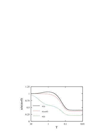
Figure 1: Shown is the electron neutrino number density corresponding to the ${\nu_{\tau}}$ mass of 5 MeV and normalized to equilibrium density $n_{0}\equiv(3\zeta(3)/2\pi^{2}){T_{\gamma}}^{3}$. The dashed line shows for comparison the unperturbed electron neutrino temperature, and the short dashed line corresponds to the ${\nu_{\tau}}$ number density. The overall decrease in the densities around ${T_{\gamma}}\sim 0.2$ MeV follows from electron-positron annihilations which increase ${T_{\gamma}}$ relative to $T_{\nu_{e}}$.

In figure 1, we plot a specific run showing the change in the electron neutrino density due to the annihilation of heavy tau neutrinos with a mass ${m_{\nu_{\tau}}}=5$ MeV. Because electron neutrinos freeze out at the temperature $T_{\rm dec}({\nu_{e}})\simeq 2.3$ MeV, their number density remains close to the equilibrium value until a few MeV. However, since the annihilation of ${\nu_{\tau}}$’s is still occurring below that temperature, there is a slight increase in the electron neutrino abundance. The excess is about 10% at ${T_{\gamma}}=0.7$ MeV, which roughly corresponds to the temperature when $n/p$-ratio freezes out. The effect of this excess is to keep $n/p$-ratio in equilibrium until a little later thereby decreasing the amount of neutrons and hence the eventual helium abundance; numerically, in the conventional units of ${{\Delta N}_{\nu}}$ this effect is found to correspond to $\simeq-4.6\delta n_{\nu_{e}}$ [30], where $\delta n_{\nu_{e}}\sim 0.1$ is the actual change in the electron neutrino number density (normalized to $n_{\rm eq}=1$) in the present example. Combined with the opposite effect on the helium abundance due to simultaneous slight increase in the energy density, the full effect of the variation in the electron neutrino density in the present example is to produce an effective negative contribution of ${\Delta N}_{\nu}^{({\nu_{e}})}\sim-0.36$ to the number of effective species; this example shows the potential importance of accounting for the electron neutrino abundance when computing the eventual bounds on masses.

We have computed the total number of effective neutrino species as a function of neutrino mass, either that of ${\nu_{\mu}}$ or ${\nu_{\tau}}$, keeping the other neutrinos massless and display the results in figure 2. We also show the result for the case where we neglect the effect on the electron neutrino density. The effect of electron neutrinos is large in the $few$ MeV region, and it does not affect the eventual bounds for the small values of ${{\Delta N}_{\nu}}$ very much. However, for larger values of ${{\Delta N}_{\nu}}$ the effect can be significant.

Including the neutrino heating, we find the following bounds on the masses as a function of ${{\Delta N}_{\nu}}$-bound: in the small mass side

$$m^{M}_{\nu}/{\rm MeV} < (0.35{\Delta N}^{1/2}_{\nu}+0.05{{\Delta N}_{\nu}}+0.59{\Delta N}^{3/2}_{\nu})\;\theta(0.15-{{\Delta N}_{\nu}}){}$$ (16)

$$+ (0.09+0.47{{\Delta N}_{\nu}}+0.83{\Delta N}^{2}_{\nu}-0.72{\Delta N}^{3}_{\nu}+0.26{\Delta N}^{4}_{\nu})\;\theta({{\Delta N}_{\nu}}-0.15){}$$

$$\equiv \phi_{M}({{\Delta N}_{\nu}}),$$

where $m_{\nu}$ is measured in MeVs and $\theta(x)$ is the step function. This bound is valid for both the muon and the tau neutrino and the error of the fit is less than 1 per cent for $0.01<{{\Delta N}_{\nu}}<2$. In the large mass side:

$$m^{M}_{\nu}/{\rm MeV} > 67.9-63.5{{\Delta N}_{\nu}}+38.7{\Delta N}^{2}_{\nu}-15.2{\Delta N}^{3}_{\nu}+2.4{\Delta N}^{4}_{\nu}{}$$ (17)

$$\equiv \Phi_{M}({{\Delta N}_{\nu}}),$$

which is accurate to better than 1 per cent up to $\Delta N_{\nu}=2.5$. For the both small and large mass limits the dependence on $\eta$ is of the order of one per cent for $\eta_{10}=1.4-3.8$.

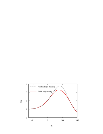
Figure 2: Shown is the effect of a massive neutrino to the nucleosynthesis as a function of its mass, expressed in terms of the effective neutrino degrees of freedom. Dotted line for the comparison shows the same result ignoring the effect on the electron neutrino density.

For example, using the limit ${{\Delta N}_{\nu}}<1.0$ from our equation (10) implies the excluded region of 0.93 MeV $<m^{M}_{\nu}<31$ MeV. A more stringent bound of ${{\Delta N}_{\nu}}<0.3$ would have led to bounds 0.31 MeV $<m^{M}_{\nu}<52$ MeV. On the other hand, given the present upper laboratory limit of ${m_{\nu_{\tau}}}<24$ MeV [15], opening up a window for a particle in the MeV range would require a nucleosynthesis bound weaker than ${{\Delta N}_{\nu}}>1.3$. Even with the considerably relaxed nucleosynthesis constraints obtained neglecting the D and ${}^{3}{\rm He}$ data [28], this does not seem very likely. Hence the nucleosynthesis bound is still to be viewed very much complementary to the laboratory bounds, excluding a stable Majorana neutrino with a mass in excess of few hundred KeV. Of course the upper limit found in equation (16) has no relevance for ${\nu_{\mu}}$ for which the laboratory bound is ${m_{\nu_{\mu}}}<160$ KeV [19]. Moreover, the lower bound coming form the nucleosynthesis can only be competitive with the laboratory bound if ${{\Delta N}_{\nu}}<0.13$.

We complete the Majorana section by noting that the nucleosynthesis bounds are cumulative; considering the effect of both masses together yields stronger constraints. We have computed these bounds by allowing both neutrinos be massive simultaneously in our code. We found that the effect in the ${\nu_{\mu}}\leftrightarrow{\nu_{\tau}}$ reaction rates due to their having simultaneously nonzero masses is small. Hence the common bounds can be directly derived from (16-17). For example the low mass limit for ${m_{\nu_{\tau}}}$ in (16) becomes

$${m_{\nu_{\tau}}}<\phi_{M}({{\Delta N}_{\nu}}-\phi^{-1}_{M}({m_{\nu_{\mu}}})).$$ (18)

A fit for the inverse function $\phi^{-1}_{M}(x)$, is explicitly given in equation (34) in the section 5.2 below. Similar expression applies for the large ${m_{\nu_{\tau}}}$ bound with $\phi_{M}$ (but not its inverse) replaced by $\Phi_{M}$ in (18). The relative error of these approximate bounds is found to be $\mbox{\raisebox{-2.58334pt}{~{}$\stackrel{{\scriptstyle<}}{{\sim}}$~{}}}5$%.

5 Dirac Case

In the case of a Dirac neutrino, one is faced with an extra complication resulting from the chirality of weak interactions; except in the very nonrelativistic limit, different helicity states have different interaction strengths. For $m\sim few$ MeV, neutrinos indeed decouple while semi-relativistic, and it behooves us to write independent evolution equations for the two helicity populations. To compare the full treatment to the usual approach which does not differentiate between the helicities and using the averaged interaction amplitudes, we note the following: First, the R-helicity population interacts much more weakly, and hence their relic density gets underestimated in the naïve approach. Secondly, the L-helicity population interacts more strongly than is assumed in the helicity averaged approach, and there is a compensating overestimation of their density. Thirdly, the situation is made more complicated by existence of $t$-channel helicity flipping interactions that mix the two species. Clearly, in order to obtain high accuracy results, a quantitative computation is required to sort out which of these effects is dominant.

Another problem is that the thermal averaging is more subtle in the Dirac case, because the spin dependent matrix elements are not Lorentz invariant. To see this explicitly, consider neutrino-neutrino scattering: in naïve approach, where one boosts the matrix element to the CM-frame, it is (see eg. (22)) of the order $\sim m^{4}_{\nu}/E^{2}$. This suppression is particular to the CM-frame however, and the true thermal average is in fact of the same order $\sim m^{2}_{\nu}$ as the other interactions that dominate in the naïve approach [20].

The technical difficulty is greatly increased by the very large number of interaction diagrams, in particular because of a large number of spin flipping $t$-channel processes that were naturally absent in the Majorana case. Finally, the lower bounds on the masses in the Dirac case are sensitive to QCD phase transition temperature [20] because the bounds, as we shall see is true even for rather large ${{\Delta N}_{\nu}}$, are saturated by an out of equilibrium excitation of right handed species below ${T_{\rm QCD}}$, the excitation process being the more effective the higher ${T_{\rm QCD}}$ is. We therefore consider large and small mass cases separately

5.1 Large mass region

We first concentrate on the large mass region $m\mbox{\raisebox{-2.58334pt}{~{}$\stackrel{{\scriptstyle>}}{{\sim}}$~{}}}{\cal O}(1)$ MeV. The distinguishing feature here is that the particles are heavy enough to have become into equilibrium below the QCD phase transition temperature so that their distributions can be described by our kinetic equilibrium approach. The region $m\mbox{\raisebox{-2.58334pt}{~{}$\stackrel{{\scriptstyle<}}{{\sim}}$~{}}}{\cal O}(1)$ MeV is not well described by the equations below and we shall return to this point later (§5.2). The complete equation network can now be written in the following form

$$\dot{n}_{{\nu_{\tau}}_{-}}+3Hn_{{\nu_{\tau}}_{-}} = \,{\sum_{\stackrel{{\scriptstyle\scriptstyle\lambda=-,+}}{{\alpha=e,{\nu_{e}},{\nu_{\mu}}}}}C({\nu_{\tau-}}{\bar{\nu}_{\tau\lambda}}\leftrightarrow\alpha\bar{\alpha})}+C_{\rm flip}^{\tau}{}$$

$$\dot{n}_{{\nu_{\tau}}_{+}}+3Hn_{{\nu_{\tau}}_{+}} = \,{\sum_{\stackrel{{\scriptstyle\scriptstyle\lambda=-,+}}{{\alpha=e,{\nu_{e}},{\nu_{\mu}}}}}C({\nu_{\tau+}}{\bar{\nu}_{\tau\lambda}}\leftrightarrow\alpha\bar{\alpha})}-C_{\rm flip}^{\tau}{}$$

$$\dot{n}_{\nu_{\mu}}+3Hn_{\nu_{\mu}} = \,\sum_{\alpha=e,\nu_{i\lambda}\neq{\nu_{\mu}}}C({\nu_{\mu}}{{\bar{\nu}}_{\mu}}\leftrightarrow\alpha\bar{\alpha}){}$$

$$\dot{n}_{\nu_{e}}+3Hn_{\nu_{e}} = \,\sum_{\alpha=e,\nu_{i\lambda}\neq{\nu_{e}}}C({\nu_{e}}{{\bar{\nu}}_{e}}\leftrightarrow\alpha\bar{\alpha}){}$$ (19)

$$\vdots \;,$$

where the dots again refer to equations (7) and (8). We included different helicity species only for tau neutrinos, because in light of the restrictive laboratory bound on muon neutrino, it does not make sense of computing BBN bounds for ${\nu_{\mu}}$ in the large mass region. The spin flip terms appearing (19) are given by

$$C_{\rm flip}^{\tau} = \sum_{\alpha=e,{\nu_{e}},{\nu_{\mu}}}\{\;C({\nu_{\tau-}}\alpha\leftrightarrow{\nu_{\tau+}}\alpha)+C({\nu_{\tau-}}\bar{\alpha}\rightarrow{\nu_{\tau+}}\bar{\alpha})\;\}{}$$ (20)

$$+ \phantom{l}\sum_{\lambda=-,+}\{\;C({\nu_{\tau-}}{\nu_{\tau\lambda}}\leftrightarrow{\nu_{\tau+}}{\nu_{\tau\lambda}})+C({\nu_{\tau-}}{\bar{\nu}_{\tau\lambda}}\leftrightarrow{\nu_{\tau+}}{\bar{\nu}_{\tau\lambda}})\;\}{}$$

$$+ 2C({\nu_{\tau-}}{\nu_{\tau-}}\leftrightarrow{\nu_{\tau+}}{\nu_{\tau+}}),$$

where the factor of 2 in the last term accounts for the fact that this interaction changes the $\nu-$number by 2 units. Generic collision terms appearing in definitions (19 - 20) are defined and normalized similarly to the equations (12-14). For example (from now on we will denote ${\nu_{\tau\lambda}}$ by ${\nu_{\lambda}}$).

$$C({\nu_{\lambda 1}}{{\bar{\nu}}_{\lambda 2}}\leftrightarrow\alpha\bar{\alpha}) \equiv \frac{1}{512\pi^{6}}(e^{z_{\lambda 1}+z_{\lambda 2}}-e^{2z_{\alpha}})\times{}$$ (21)

$$\times\int{\cal D}\Phi_{\{z_{i}\}}\int_{0}^{2\pi}{\rm d}\phi\sum_{\rm spin}\mid{\cal M}({\nu_{\lambda 1}}{{\bar{\nu}}_{\lambda 2}}\rightarrow\alpha\bar{\alpha})\mid^{2},$$

where we dropped the symmetry factors which equal to unity and the annihilation matrix element is given by

$$\sum_{\rm spin}\mid{\cal M}({\nu_{\lambda 1}}{{\bar{\nu}}_{\lambda 2}}\rightarrow\alpha\bar{\alpha})\mid^{2} = 16G_{F}^{2}\left\{(c_{V\alpha}^{2}+c_{A\alpha}^{2})\left(K_{\lambda 1}\cdot p_{3}K_{-\lambda 2}\cdot p_{4}\right)\right.{}$$ (22)

$$\phantom{Han}\left.-\frac{1}{2}(c_{V\alpha}^{2}-c_{A\alpha}^{2})\,m_{\alpha}^{2}\>K_{\lambda 1}\cdot K_{-\lambda 2}\right\}.$$

Here, in order to condense the notation, we dropped the terms that vanish, and combined others that are equal under the integration; similar simplifications are made in other matrix elements following below. The coefficients $c_{V\alpha}$ and $c_{A\alpha}$ have been defined in section 4 and the 4-vector $K^{\mu}_{\lambda}\equiv k^{\mu}-m_{\nu}s^{\mu}_{\lambda}$ is related to the ‘spin vector’ $s^{\mu}_{\lambda}$ of $i$th neutrino and can be written as

$$K^{\mu}_{\lambda}=(E-\lambda(E^{2}-m^{2}_{\nu})^{1/2})(1;-\lambda{\bf k}/k).$$ (23)

Other matrix elements appearing in the collision terms above include the $t$-channel scattering off the electrons and other neutrinos and their antiparticles. Under the assumption that the chemical potentials are small ($\ll 1$) the distribution functions for particles and antiparticles are equivalent, and we can add their contributions under the integral:

$$\sum_{\rm spin,\;\beta=\alpha,\bar{\alpha}}\mid{\cal M}({\nu_{\lambda 1}}\beta\rightarrow{\nu_{\lambda 2}}\beta)\mid^{2} = 16G_{F}^{2}\left\{(c_{V\alpha}^{2}+c_{A\alpha}^{2})\left(K_{\lambda 1}\cdot p_{2}K_{\lambda 1}\cdot p_{4}+K_{\lambda 1}\cdot p_{4}K_{\lambda 3}\cdot p_{2}\right)\phantom{\frac{1}{2}}\right.{}$$ (24)

$$\phantom{Ham}\left.-(c_{V\alpha}^{2}-c_{A\alpha}^{2})\,m_{\alpha}^{2}\>K_{\lambda 1}\cdot K_{\lambda 3}\right\}.$$

Finally, self scatterings can all be derived from the matrix elements

$$\mid{\cal M}(\nu_{\lambda 1}\bar{\nu}_{\lambda 2}\rightarrow\nu_{\lambda 3}\bar{\nu}_{\lambda 4})\mid^{2}\;=\;8G_{F}^{2}\;K_{\lambda 1}\cdot K_{-\lambda 4}K_{\lambda 2}\cdot K_{-\lambda 3}$$ (25)

and

$$\mid{\cal M}(\nu_{\lambda 1}\nu_{\lambda 2}\rightarrow\nu_{\lambda 3}\nu_{\lambda 4})\mid^{2}\;=\;8G_{F}^{2}\;K_{\lambda 1}\cdot K_{\lambda 2}K_{\lambda 3}\cdot K_{\lambda 4}.$$ (26)

The symmetry factors appearing in the collision integrals are equal to one everywhere except the reactions corresponding to (26). There, the symmetry factor is one half, because of the degeneracy in either initial or in final state, except for the reaction ${\nu_{\tau-}}{\nu_{\tau-}}\rightarrow{\nu_{\tau+}}{\nu_{\tau+}}$, where the symmetry factor is $1/4$. Note that this reaction changes ${\nu_{\tau-}}$ number by two units, but that was explicitly taken into account in the equation (20).

The collision integrals of the massless ${\nu_{e}}$ and ${\nu_{\mu}}$ appearing in (19) are obtained from the Majorana matrix element (15) in the limit $m_{\nu}=0$. Equations (15,22-26) exhaust the list of interactions relevant for the evolution of the neutrino ensembles. Each of the matrix elements (15, 22-26) is a polynomial at most of second order of the cosine of the acoplanarity $\phi$. We integrate over $\phi$ analytically, after which the remaining 4-dimensional integral is performed numerically using the special frame introduced in the appendix A. In figure 3 we show the temperature dependence of the annihilation and flip rates $\Gamma_{\nu_{\lambda\pm}}$ and $\Gamma_{\rm flip}$, defined by (see the appendix A) $\Gamma_{i}=\sum_{j}n_{j}\langle v_{\rm M\o l}\sigma(ij\rightarrow kl)\rangle$ for the particular case of ${m_{\nu_{\tau}}}=5$ MeV along with the Hubble expansion rate. One sees how the right helicity population drops from the equilibrium much earlier than left helicity states. Yet both states are in complete equilibrium until well below the QCD phase transition temperature ${T_{\rm QCD}}\sim few$ 100 MeV.

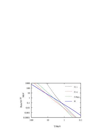
Figure 3: Shown are the total annihilation rates $\Gamma_{{\nu_{\lambda\pm}}}$ and the total flip rate $\Gamma_{\rm flip}$ (see the text) in comparison with the Hubble expansion rate $H(T)$.

In figure 4, we show a particular example of the evolution of the neutrino energy densities as a function of time. While negative and positive helicity populations have different densities from each other, their average comes close to that obtained in the helicity averaged approach.

Figure 4: Shown is the evolution of the energy densities of ${\nu_{\tau-}}$, ${\nu_{\tau+}}$ and ${\nu_{e}}$ corresponding to a run of the code with ${m_{\nu_{\tau}}}=20$ MeV and normalized to $\rho_{0}=7\pi^{2}T^{4}/240$. Also shown is the energy density corresponding to ${\nu_{\tau}}$ in the helicity averaged approximation.

In figure 5, we show the change in the helium abundance in the Dirac case for $m^{D}_{\nu_{\tau}}\mbox{\raisebox{-2.58334pt}{~{}$\stackrel{{\scriptstyle>}}{{\sim}}$~{}}}1$ MeV. We did our computations also using the helicity averaged approach. The final results turned out to be very close to the full solution, in particular in the region of interest for nucleosynthesis bounds. While one might have expected this result on qualitatively, the quantitative proof only could follow from a numerical calculation.

We find that the nucleosynthesis bound on the ${\nu_{\tau}}$ mass is fitted to an accuracy of one per cent in the range $0<{{\Delta N}_{\nu}}<2.5$ by:

$$m^{D}_{\nu_{\tau}}/{\rm MeV} < 37.8-26.9{{\Delta N}_{\nu}}+21.3{\Delta N}^{2}_{\nu}-15.5{\Delta N}^{3}_{\nu}+6.3{\Delta N}^{4}_{\nu}-0.1{\Delta N}^{5}_{\nu}{}$$ (27)

$$\equiv \Phi_{D}({{\Delta N}_{\nu}}).$$

This is the main result of this subsection. One observes that the nucleosynthesis constraint allows a stable Dirac neutrino just below the laboratory bound ${m_{\nu_{\tau}}}<24$ MeV, given that ${{\Delta N}_{\nu}}>0.8$. This seems to be admissible given the relaxed constraint following from the equation (10); indeed, the bound ${{\Delta N}_{\nu}}<1.0$ gives the constraint $m^{D}_{\nu_{\tau}}>22$ MeV. More stringent bound of ${{\Delta N}_{\nu}}<0.3$ would lead to $m^{D}_{\nu_{\tau}}>31$ MeV. Our result (27) differs noticeably from the previous computations and fall roughly in between the results obtained in [2] and [5] given the particular values for the bound for ${{\Delta N}_{\nu}}$ used therein.

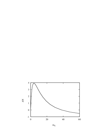
Figure 5: Shown is the effective number of degrees of freedom for a Dirac tau neutrino.

5.2 Small mass region

The mass of a neutrino is considered ‘small’ if the R-helicity population is out of equilibrium below ${T_{\rm QCD}}$. Even in this case however, a significant amount of R-helicity states may be produced by out of equilibrium spin flip processes [20]. We shall see below that even for very large ${{\Delta N}_{\nu}}$, the lower limit in the exclusion region indeed is saturated by a mass for which R-helicity states are out of equilibrium.

In the small mass region it does not make sense to describe the R-helicity system with the distribution function (2). Instead, noting that the R-helicity states are produced from an equilibrium ensemble of left helicity states through very mildly energy dependent spin flip interactions, the increments in R-helicity population appear with a local (in time) equilibrium density characterized by the excitation temperature $T(t_{\rm ex})$. Provided that the backscattering is not very efficient (to be checked a posteriori), one can compute the total energy density in the right handed species very accurately by including the dilution due to entropy production subsequent to excitations. This program was carried out in the reference [20]. Here we stress that the underlying assumption of no backscattering and hence the bounds are valid for surprisingly large values of ${{\Delta N}_{\nu}}$. To this end we extend the treatment of [20] by including a simple but accurate model of backscattering. We also point out and correct an inaccurate treatment of the effect of a mass of a neutrino for the nucleosynthesis in the final stages of the analysis of [20]. The corrected analysis turns out to give bounds roughly 30 per cent more stringent than those of ref. [20].

We will write down the starting point of our analysis using the results obtained in ref. [20]. Because the spin flip processes involving only one right helicity state at the time are by far the dominant interactions here, an equation which simply models the back scatterings can be written as

$$\dot{\rho}_{\nu}+4H\rho_{\nu}=\frac{G_{F}^{2}m_{\nu}^{2}}{2\pi^{5}}{\hat{K}}_{\rm eff}T^{7}\;{\cal C}_{\nu}(T)\;(1-\rho/\rho_{\rm eq})$$ (28)

where $\rho_{\rm eq}=7\pi^{2}T^{4}/240$ is the equilibrium energy density of massless neutrinos, ${\hat{K}}\simeq 16.52$ includes counting over all channels the Fermi-Dirac correction due to the statistics of the L-helicity particles and the functions ${\cal C}_{i}$ are given by [20]

$${\cal C}_{\mu}(T) = 1+0.81d_{\mu}(T)+3.71\times 10^{-2}\left((\frac{f_{\pi^{0}}}{T})^{2}z_{0}^{4}K_{2}(z_{0})\right.$$

$$\phantom{hanna}\left.+(\frac{f_{\pi^{\pm}}}{T})^{2}z_{\pm}^{4}(1-y^{2})\{(1+y^{2})K_{2}(z_{\pm})-y^{2}K_{0}(z_{\pm})\}\right)$$

$${\cal C}_{\tau}(T) = 1+0.06d_{\tau}(T)+3.71\times 10^{-2}(\frac{f_{\pi^{0}}}{T})^{2}z_{0}^{4}K_{2}(z_{0})$$ (29)

where the functions $d_{i}(T)$ express the nontrivial temperature dependence (deviation from the $T^{7}$-law) of the scattering collision term due to the scatterings off muons. The terms involving the modified Bessel functions $K_{i}(z)$ correspond to pion decays with, $z_{0}\equiv m_{\pi^{0}}/T$, $z_{\pm}\equiv m_{\pi^{\pm}}/T$, $y\equiv m_{\pi^{\pm}}/m_{\mu}$ and $f_{\pi^{0}}\simeq 93$ MeV and $f_{\pi^{\pm}}\simeq 128.7$ MeV. Equation (28) is easily integrated along with the equation (8) to yield a double integral expression for the relative energy density $r\equiv\rho/\rho_{\rm eq}$

$$r(x) = \int_{x}^{1}{\rm d}x^{\prime}(\frac{h_{I}(x)}{h_{I}(x^{\prime})})^{4/3}A(x^{\prime})\exp\int_{x}^{x^{\prime}}{\rm d}x^{\prime\prime}A(x^{\prime\prime})$$ (30)

$$+ {r_{\rm QCD}}\;(\frac{h_{I}(x)}{h_{I}(x_{\rm QCD})})^{4/3}\exp\int_{1}^{x}{\rm d}x^{\prime}A(x^{\prime}),$$

where ${r_{\rm QCD}}=(17.25/60)^{4/3}\simeq 0.19$ is the diluted energy density of the equilibrium ensemble of R-helicity population decoupled above the QCD phase transition, $x\equiv T/{T_{\rm QCD}}$, and

$$A(x)\simeq 2.88\;m_{\nu}^{2}\;{T^{100}_{\rm QCD}}\;(\frac{10.75}{g_{*}(x)})^{1/2}(1+\frac{x}{3h_{I}}\frac{{\rm d}h_{I}}{{\rm d}x})\;{\cal C}_{\nu}(x),$$ (31)

where ${T^{100}_{\rm QCD}}\equiv{T_{\rm QCD}}/100$ MeV, $x\equiv T/{T^{100}_{\rm QCD}}$ and $m_{\nu}$ is in units MeV. Expression (30) obviously reduces to those of [20] when backscattering is neglected. We computed the relevant value of the function $r$ during the nucleosynthesis, $r(0)$, for a large set of parameters $m_{\nu}$ and ${T_{\rm QCD}}$ and found that it is to a reasonable approximation

$$r(0)\simeq r^{\prime}_{\rm QCD}e^{-\Delta r_{i}}+(1-e^{-\Delta r_{i}}),$$ (32)

where $r^{\prime}_{\rm QCD}\simeq 0.1$ and

$$\Delta r_{\mu}=(2.89+2.25{T^{100}_{\rm QCD}})\;m^{2}_{\nu_{\mu}}$$

$$\Delta r_{\tau}=(1.29+1.34{T^{100}_{\rm QCD}})\;m^{2}_{\nu_{\tau}}$$ (33)

The accuracy is no worse than 3 per cent for ${T_{\rm QCD}}=100-200$ MeV and ${{\Delta N}_{\nu}}<1.5$, which corresponds to the whole region of applicability of the final result. For ${T_{\rm QCD}}=300-400$ it undershoots by about 10 per cent at large ${{\Delta N}_{\nu}}\mbox{\raisebox{-2.58334pt}{~{}$\stackrel{{\scriptstyle>}}{{\sim}}$~{}}}1.5$. It should be noted that due to the mass effects, a single neutrino with an equilibrium density effectively corresponds to $1+f(m)$ species. Using the nucleosynthesis code we have computed a fit for this function. For moderately small masses $m_{\nu}\mbox{\raisebox{-2.58334pt}{~{}$\stackrel{{\scriptstyle<}}{{\sim}}$~{}}}0.6$ MeV, it in fact coincides with the function $\phi^{-1}(m_{\nu})$ for the number of effective degrees of freedom for the small mass majorana neutrinos, defined in equation (16):

$$f(m)=\phi^{-1}_{M}(m) = (-18.6m^{3}+7.9m^{2}+0.02m)\;\theta(0.15-m){}$$ (34)

$$+ (0.007m^{4}-0.019m^{3}+0.237m^{2}+1.40m-0.09)\;\theta(m-0.15).$$

The function $f(m)$ defined above differs considerably from the fit $f(m^{2})$ used in its place in ref. [20]. Using the approximation (32) we are finally led to the constraint equation

$$f(m)+(1+f(m))(r^{\prime}_{\rm QCD}e^{-\Delta r_{i}}+(1-e^{-\Delta r_{i}}))<{{\Delta N}_{\nu}}.$$ (35)

We plot the bound for the tau neutrino in figure 6 for ${T_{\rm QCD}}=100-400$ MeV with our improved fit function $f(m)$ and using the exact expression (30) for $r(0)$. We also show the value of $r(0)$ to underline how the effective value for ${{\Delta N}_{\nu}}$ greatly exceeds $r(0)$ for even moderate masses. This is the reason why the backscattering correction is so small (we find it is typically at most 10 per cent for ${{\Delta N}_{\nu}}\mbox{\raisebox{-2.58334pt}{~{}$\stackrel{{\scriptstyle<}}{{\sim}}$~{}}}1.5$).

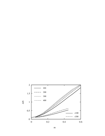
Figure 6: Shown is the bound on the Dirac ${\nu_{\tau}}$ mass as a function of the nucleosynthesis constraint ${{\Delta N}_{\nu}}$ for ${T_{\rm QCD}}=100-400$ MeV The two short lines show the function $r(0)$ for ${T_{\rm QCD}}=100-200$ MeV.

There is a slight inaccuracy in the derivation above that goes over the stated approximations. Namely, we have computed the mass effect of the excited right handed population by multiplying by $f(m)$ their fraction of the energy density $r$. It is clear however that this mass effect actually depends on the relative number density $n$ instead. To correct for this inaccuracy would require computing also $n$ in a way similar we found $r$ above. This would merely require re-evaluating the collision terms and correcting the power for the dilution factor $4/3\rightarrow 1$ in equation (30). We will not do so here, because the error made is very small. Indeed, using the equation (32) it is easy to show that the relative error (undershoot) in ${{\Delta N}_{\nu}}$ is generously bracketed by $\delta({{\Delta N}_{\nu}})<((a-1)r^{\prime}_{\rm QCD}e^{-\Delta r}+(b-1)(1-e^{-\Delta r}))f(m)\mbox{\raisebox{-2.58334pt}{~{}$\stackrel{{\scriptstyle<}}{{\sim}}$~{}}}0.04{{\Delta N}_{\nu}}$, in the mass range of interest ($a\equiv(60/10.75)^{1/3}$ and $b\equiv(17.25/10.75)^{1/3}$). Moreover, this error tends to cancel the error made by the approximation (32).

In case of the muon neutrino, our bound becomes competitive with the laboratory bound of ${m_{\nu_{\mu}}}<160$ KeV, when ${{\Delta N}_{\nu}}<0.39$ (0.44) for ${T_{\rm QCD}}=100$ (200) MeV. Since we are finding that the function $f(m)$ was inaccurately estimated in ref. [20] we give for comparison the correct bounds for the values of ${T_{\rm QCD}}$ and ${{\Delta N}_{\nu}}<0.3$ discussed there:

$$m_{\nu_{\mu}}\>\mbox{\raisebox{-2.58334pt}{~{}$\stackrel{{\scriptstyle<}}{{\sim}}$~{}}}\>\left\{\begin{array}[]{lll}&130~{}{\rm KeV}&\;\;T_{QCD}=100~{}{\rm MeV}\\ &120~{}{\rm KeV}&\;\;T_{QCD}=200~{}{\rm MeV}\end{array}\right.\,$$

$$m_{\nu_{\tau}}\>\mbox{\raisebox{-2.58334pt}{~{}$\stackrel{{\scriptstyle<}}{{\sim}}$~{}}}\>\left\{\begin{array}[]{lll}&150~{}{\rm KeV}&\;\;T_{QCD}=100~{}{\rm MeV}\\ &140~{}{\rm KeV}&\;\;T_{QCD}=200~{}{\rm MeV.}\end{array}\right.$$

For ${{\Delta N}_{\nu}}<1.0$, these limits become:

$$m_{\nu_{\mu}}\>\mbox{\raisebox{-2.58334pt}{~{}$\stackrel{{\scriptstyle<}}{{\sim}}$~{}}}\>\left\{\begin{array}[]{lll}&310~{}{\rm KeV}&\;\;T_{QCD}=100~{}{\rm MeV}\\ &290~{}{\rm KeV}&\;\;T_{QCD}=200~{}{\rm MeV}\end{array}\right.\,$$

$$m_{\nu_{\tau}}\>\mbox{\raisebox{-2.58334pt}{~{}$\stackrel{{\scriptstyle<}}{{\sim}}$~{}}}\>\left\{\begin{array}[]{lll}&370~{}{\rm KeV}&\;\;T_{QCD}=100~{}{\rm MeV}\\ &340~{}{\rm KeV}&\;\;T_{QCD}=200~{}{\rm MeV.}\end{array}\right.$$

Before concluding, we discuss the connection between the computations in the high mass and the low mass regions. It should be obvious that when the function $r(0)$ is close to 1, one actually enters the region where the kinetic-equilibrium treatment employed at the high mass region becomes valid. However, one would expect that the connection of the low and high mass solutions is not completely smooth, because close to the crossing point the right helicity population is not quite in complete equilibrium, nor completely out of equilibrium ($r_{QCD}$ is bigger than assumed in the low mass treatment). Hence it is difficult to improve the computation quantitatively without a detailed knowledge of the QCD phase transition dynamics. We conclude that the bound (35) should be trusted until about ${{\Delta N}_{\nu}}\sim 1.0$, above which there may be large (few tens of per cents) uncontrolled uncertainties in the results.

6 Conclusions

In conclusion, we have carefully computed the mass bounds on the stable Majorana and Dirac neutrinos arising from nucleosynthesis constraints. We also discussed in detail how nucleosynthesis constraints on particle physics models arise, and how (and to what extent) they can generically be modeled through the effective number of degrees of freedom. In our computation of the mass bounds we included the effects of heating of the electron neutrino system as a result of the annihilations below the ${\nu_{e}}$ freeze-out temperature and the effect of chirality in the weak interactions on the evolution of different helicity components in the case of a Dirac neutrino. We also computed the bounds for the case in which both ${\nu_{\mu}}$ and ${\nu_{\tau}}$ are massive simultaneously, resulting in stronger constraints. Most importantly, we computed all bounds as functions of the actual nucleosynthesis constraint on the effective number of neutrino degrees of freedom ${{\Delta N}_{\nu}}$, except in the case of light Dirac neutrinos, where nevertheless an implicit function of a form $\phi_{D}({{\Delta N}_{\nu}},m_{\nu}$, ${T_{\rm QCD}})=0$ was derived for the bound. We claim that in all our bounds, the theoretical uncertainty is negligible and therefore realistic bounds, or estimates of the uncertainties in the bounds can be obtained solely on the basis of a separate analysis of the determination of the bound on ${{\Delta N}_{\nu}}$.

Appendix A Phase space integrals

In this appendix we define the phase space co-ordinate system we employed in our computations and write down the matrix element in terms of these variables in a couple examples. We took the independent variables to be the magnitude of the two 3-momenta of the incoming states, $k_{1}$ and $k_{2}$, energy of one of the outgoing states $E_{q2}$, the angle between the incoming states $\theta$ and the acoplanarity angle $\phi$ between the collision planes. In terms of these variables relevant 4-momenta have the expressions (we are using the same expression for the 4-momentum and the magnitude of the corresponding 3-momentum; what is meant in each occasion should be obvious however)

$$k_{1} = (E_{k1};k_{1}\sin\theta_{1},0,k_{1}\cos\theta_{1}){}$$

$$k_{2} = (E_{k2};-k_{2}\sin\theta_{2},0,k_{2}\cos\theta_{2}){}$$

$$p_{4} = (E_{p4};p_{4}\sin\theta_{K}\cos\phi,p_{4}\sin\theta_{K}\sin\phi,p_{4}\cos\theta_{K}),$$ (36)

where the angles are defined as

$$\cos\theta_{1} = (k_{1}+k_{2}\cos\theta)/\kappa{}$$

$$\cos\theta_{2} = (k_{2}+k_{1}\cos\theta)/\kappa{}$$

$$\cos\theta_{K} = \frac{1}{\kappa Q_{1}}\left(E_{p4}(E_{k1}+E_{k2})-E_{k1}E_{k2}+k_{1}k_{2}\cos\theta\phantom{\frac{1}{2}}\right.{}$$ (37)

$$\phantom{Hannatyt}\left.-\frac{1}{2}(m_{1}+m_{2}+m_{4}-m_{3})\right).$$

and $\kappa=({\bf k}_{1}+{\bf k}_{2})^{2}$ (cf. equation (14)). In terms of these variables the matrix element (15) in the Majorana case becomes

$$\int{\rm d}\phi|{\cal M}|^{2} = 128\pi G_{F}^{2}\left\{(c_{V\alpha}^{2}+c_{A_{\alpha}}^{2})\left(s^{2}/2-2s(E_{k1}E_{p4}+k_{1}p_{4}\cos\theta_{1}\cos\theta_{K})\right.\right.{}$$ (38)

$$\phantom{Hannaty}\left.\left.+4E_{k1}^{2}E_{p4}^{2}-8E_{k1}E_{p4}k_{1}p_{4}\cos\theta_{1}\cos\theta_{K}\right.\right.{}$$

$$\phantom{Hannaty}\left.\left.+2k_{1}^{2}p_{4}^{2}\left(2\cos\theta_{1}^{2}\cos\theta_{K}^{2}+\sin\theta_{1}^{2}\sin\theta_{K}^{2}\right)-m_{\nu_{\beta}}^{2}(s-2m_{\alpha}^{2})\right)\right.{}$$

$$\phantom{Hanna}\left.+\;(c_{V\alpha}^{2}-c_{A_{\alpha}}^{2})\,m_{\alpha}^{2}\>\left(s-6m_{\nu_{\beta}}^{2}\right)\right\},$$

where $s=2E_{k1}^{2}E_{k2}-2k_{1}k_{2}\cos\theta+m_{i1}^{2}+m_{i2}^{2}$. We have checked numerically that when integrated over the phase space in the Maxwell-Boltzmann approximation, the matrix element (38) reproduces the much simpler thermal average over the invariant cross section [22]

$$\langle v_{\rm M\o l}\sigma\rangle \equiv \frac{1}{512\pi^{6}n_{1}n_{2}}\times\int{\cal D}\Phi_{\{0\}}\int_{0}^{2\pi}{\rm d}\phi\sum_{\rm spin}\mid{\cal M}(\nu_{\beta}\bar{\nu}_{\beta}\rightarrow\alpha\bar{\alpha}\mid^{2}\;S_{\rm in}S_{\rm fi}{}$$ (39)

$$\stackrel{{\scriptstyle\scriptstyle\rm MB}}{{\mapsto}} {1\over 8m^{4}TK_{2}^{2}({m\over T})}\int_{4m^{2}}^{\infty}{\rm d}s\sqrt{s}(s-4m^{2})K_{1}({\sqrt{s}\over T})\sigma_{\rm CM}(s),$$

where the cross section is easily obtained by integrating the matrix element (15)

$$\sigma_{\rm CM}(s) = \frac{G_{F}^{2}}{2\pi s}\frac{v_{f}}{v_{i}}\left\{(c_{V\alpha}^{2}+c_{A_{\alpha}}^{2})\left(s^{2}(1+\frac{1}{3}v_{i}^{2}v_{f}^{2})-4m_{\nu}^{2}(s-2m_{\alpha}^{2})\right)\right.{}$$ (40)

$$\left.\phantom{\frac{G_{F}^{2}}{\pi}a}+4(c_{V\alpha}^{2}-c_{A_{\alpha}}^{2})m_{\alpha}^{2}(s-6m_{\nu}^{2})\right\}.$$

Similar checking is not directly possible in the Dirac case, because there the matrix element is not invariant and one does not expect the helicity amplitudes to reduce to the simple expression (39). However, the helicity summed amplitude is of course again an invariant and we undertook to check in every case separately that when summed over initial state helicities our thermal averages again did reproduce the simpler results (39) over the total scattering cross section in the Maxwell-Boltzmann limit.

References

- [1] T.P. Walker, G. Steigman, D.N. Schramm, K.A. Olive and K. Kang, Ap. J. 376 (1991) 51.
- [2] E.W. Kolb et. al. , Phys. Rev. Lett. 29, 533 (1991) and references therein.
- [3] G.M. Fuller and R.A. Malaney, Phys. Rev. D43, 309 (1991).
- [4] K. Enqvist and H. Uibo, Phys. Lett. B301, 376 (1993).
- [5] A.D. Dolgov and I.Z. Rothstein, Phys. Rev. Lett. 71, 476 (1993).
- [6] M. Kawasaki et.al. Nucl. Phys. B419, 105 (1994).
- [7] S. Dodelson G. Gyuk and M.S. Turner, Phys. Rev. D49, 5068 (1994).
- [8] K.A. Olive, D.N. Schramm, G. Steigman, and T.P. Walker, Phys. Lett. B236, 454 (1990).
- [9] K.A. Olive and G. Steigman, Ap. J. Supp. 97 (1995) 49.
- [10] P.J. Kernan and L.M. Krauss, Phys. Rev. Lett. 72, 3309 (1994); L.M. Krauss and P.J. Kernan Phys. Lett. B347, 347 (1995).
- [11] N. Hata, R.J. Scherrer, G. Steigman, D. Thomas, T.P. Walker, S. Bludman and P. Langacker, Phys. Rev. Lett. 75 3977 (1995).
- [12] G.C. Copi, D. Schramm and M.S. Turner, Ap.J. 455 L95 (1995); and astro-ph/9508029.
- [13] K.A. Olive and G. Steigman, Phys. Lett. B354, 357 (1995).
- [14] B.D. Fields and K.A. Olive, UMN-TH-1407/95, hep-ph/9508344, Phys. Lett. B (in press); B.D. Fields, astro-ph/9512044, Astropyhs. J. (in press).
- [15] ALEPH collaboration, D. Buskulic et. al. Phys. Lett. B349, 585 (1995).
- [16] J. Bernstein, L.S. Brown and G. Feinberg, Phys. Rev. D32, 3261 (1992).
- [17] A.D. Dolgov and K. Kainulainen, Nucl. Phys. B402, 349 (1993).
- [18] K. Enqvist, K. Kainulainen and V. Semikoz, Nucl. Phys. B374, 392 (1992).
- [19] K. Assamsan et. al. Reoprt No. PSI-PR-94-29.
- [20] A.D. Dolgov, K. Kainulainen and I.Z. Rothstein, Phys. Rev. D51, 4129 (1995).
- [21] G. Steigman, Ann. Rev. Nucl. Part. Sci. 29, 313 (1979); R.J. Sherrer and M.S. Turner, Phys. Rev. D33, 1585 (1986); K. Griest and D. Seckel, Nucl. Phys. B283, 681 (1987).
- [22] P. Gondolo and G. Gelmini, Nucl. Phys. B360, 145 (1992).
- [23] S. Weinberg, Gravitation and Cosmology, John Wiley and Sons, New York.
- [24] J. Bernstein, Kinetic theory in the expanding universe, Cambridge University Press, Cambridge.
- [25] I. Iben, and J.W. Truran, Ap. J. 220 (1978) 980.
- [26] R.T. Rood, T.M. Bania, and T.L. Wilson, Nature 355 (1992) 618; R.T. Rood, T.M. Bania, T.L. Wilson, and D.S. Balser, in the Light Element Abundances, Proceedings of the ESO/EIPC Workshop, ed. P. Crane, (Berlin:Springer, 1995), p. 201
- [27] K.A. Olive, R.T. Rood, D.N. Schramm, J.W. Truran, and E. Vangioni-Flam, Ap. J. 444 (1995) 680; S.T. Scully, M. Cassé, K.A. Olive, D.N. Schramm, J.W. Truran, and E. Vangioni-Flam, astro-ph/0508086 (1995), Ap. J. (in press).
- [28] B.D. Fields, K. Kainulainen and K.A. Olive, in preparation.
- [29] Particle Data Group, K. Hikasa, et.al. Phys. Rev. D45 (1992)
- [30] K. Enqvist, K. Kainulainen and M. Thomson, Nucl. Phys. B373, 498 (1992).