Hadronic $\psi$ production calculated in the NRQCD factorization formalism

Sean Fleming Department of Physics, University of Wisconsin, Madison, WI 53706    Ivan Maksymyk Theory Group, Department of Physics, University of Texas, Austin, TX 78712
Abstract

The NRQCD factorization formalism of Bodwin, Braaten, and Lepage prescribes how to write quarkonium production rates as a sum of products of short-distance coefficients times non-perturbative long-distance NRQCD matrix elements. We present, in the true spirit of the factorization formalism, a detailed calculation of the inclusive cross section for hadronic $\psi$ production. We find that in addition to the well known color-singlet production mechanisms, there are equally important mechanisms in which the $c\bar{c}$ pair that forms the $\psi$ is initially produced in a color-octet state, in either a ${}^{3}S_{1}$, ${}^{1}S_{0}$, ${}^{3}P_{0}$ or ${}^{3}P_{2}$ angular-momentum configuration. In our presentation, we emphasize the β€œmatching” procedure, which allows us to determine the short-distance coefficients appearing in the factorization formula. We also point out how one may systematically include relativistic corrections in these calculations.

††preprint: MADPH-95-922 UTTG-13-95 hep-ph/9512320

I Introduction

Bodwin, Braaten, and Lepage (BBL) have devised a rigorous factorization formalism that places the calculation of inclusive quarkonium annihilation and production on a solid theoretical foundation [1]. Their approach is based on nonrelativistic quantum chromodynamics (NRQCD) [2]. This is an effective field theory involving an expansion in derivatives, constructed so as to be equivalent to QCD for non-relativistic heavy quark-anti-quark scattering, to any desired order in the relative three-momentum of the heavy quarks. In Ref. [1], it is shown that the production rate for a quarkonium bound state $H$ can be written using a factorization formula, which is a sum of products, having the form

$$\sigma(H)=\sum_{n}\frac{F_{n}}{m_{Q}^{d_{n}-4}}\langle 0|{\cal O}^{H}_{n}|0\rangle\;.$$

The β€œshort-distance” coefficients $F_{n}$ are obtainable in perturbation theory as a series in $\alpha_{s}(m_{Q})$, and can be determined through a calculation of the production rate of an on-shell $Q\bar{Q}$ pair. As to the NRQCD matrix elements $\langle 0|{\cal O}^{H}_{n}|0\rangle$, they encode analytically uncalculable β€œlong-distance” effects such as the hadronization of a $Q\bar{Q}$ pair into bound quarkonium. The index $n$ labels color and angular-momentum quantum numbers, as well as the order in the NRQCD momentum expansion. In contrast to previous approaches, the BBL formalism establishes a framework within which it is possible to properly handle soft gluon effects and systematically incorporate relativistic corrections.

The size of any NRQCD matrix element can be estimated as some power of the small parameter $v$, the typical velocity of the heavy quarks in the bound state. (For charmonium, $v^{2}\approx 0.3$.) Combining $v$-scaling estimates with knowledge of the size of the $F_{n}$ (for which the order in $\alpha_{s}(m_{Q})$ is easily determined), one can deduce the relative importance of the various terms in the factorization formula. Keeping only those terms warranted by experimental precision, one can cast each observable as a sum involving only a small number of NRQCD matrix elements. In this way, the important NRQCD matrix elements can be empirically determined by fitting a set of factorization formulæ to a body of experimental data.

In this paper we carefully present an example of a calculation in the factorization formalism. The quantity that we choose to calculate is the inclusive hadronic $\psi$ production cross section, since it is needed for a complete theoretical description of $\psi$ production at fixed target experiments. Using $v$-scaling rules alluded to above, we find that in addition to previously calculated color-singlet contributions, there exist equally important contributions involving the production of $c\bar{c}$ pairs in a color-octet state. The color-octet processes which turn out to be important in hadronic $\psi$ production are those in which the heavy quark pair is produced in either a ${}^{3}S_{1}$, ${}^{1}S_{0}$, ${}^{3}P_{0}$ or ${}^{3}P_{2}$ angular-momentum state.

Taking the octet-mechanism contributions to hadronic $\psi$ production as an illustrative example, we present a systematic procedure for determining the short-distance coefficients $F_{n}$ appearing in the factorization formula. This procedure involves the calculation of rates for the production of $Q\bar{Q}$ pairs with specific color and angular-momentum quantum numbers. These production rates are expressed as an integral over ${\bf q}$, the relative three-momentum of the $Q$ and $\bar{Q}$ in the $Q\bar{Q}$ rest frame, with the integrand being a Taylor expansion in ${\bf q}^{2}/m_{c}^{2}$. The production rates are calculated both in full QCD and in NRQCD, and then the results are β€œmatched,” allowing a determination of the $F_{n}$.

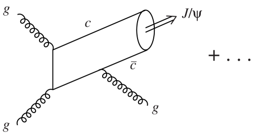
The Feynman diagrams for the leading color-singlet hadronic $\psi$ production subprocesses are shown in Figure 1. However, we do not calculate these leading color-singlet contributions since they have already been treated using the color-singlet-wavefunction modelΒ [3]. For calculations at leading order in $v^{2}$, the results of this latter approach can be readily transformed into the factorization formalism language.

II NRQCD factorization approach

A Factorization Formula

As was stated in the introduction, the NRQCD factorization formalism prescribes a means of expressing the inclusive production rate of a heavy quarkonium meson $H$ using a factorization formula, which is a sum of products of the form

$$\sigma(A+B\to H+X)=\sum_{n}\;\frac{F_{n}}{m_{Q}^{d_{n}-4}}\;\langle 0|{\cal O}^{H}_{n}|0\rangle\;.$$ (1)

The short-distance coefficients $F_{n}$ can be calculated using Feynman diagram methods. Each $F_{n}$ can be expressed as a perturbation series in $\alpha_{s}(m_{Q})$. The appropriate scale for the process is $m_{Q}$ since this is the scale that is associated with the production of a $Q\bar{Q}$ pair with small relative momentum.

The NRQCD matrix elements $\langle 0|{\cal O}^{H}_{n}|0\rangle$ are of the form

$$\langle 0|{\cal O}^{H}_{n}|0\rangle=\sum_{X}\sum_{m_{J}}\;\langle 0|{\cal K}_{n}|H_{m_{J}}+X\rangle\;\langle H_{m_{J}}+X|{\cal K}^{\prime}_{n}|0\rangle\;,$$ (2)

where 𝒦nsubscript𝒦𝑛{\cal K}_{n} and 𝒦nβ€²subscriptsuperscript𝒦′𝑛{\cal K}^{\prime}_{n} are bilinear heavy-quark field operators; 𝒦nsubscript𝒦𝑛{\cal K}_{n} may take forms such as Ο‡β€ β€‹Οˆsuperscriptπœ’β€ πœ“\chi^{\dagger}\psi, χ†​σiβ€‹Οˆsuperscriptπœ’β€ superscriptπœŽπ‘–πœ“\chi^{\dagger}\sigma^{i}\psi, Ο‡β€ πˆβ‹…πƒβ†”Οˆ\chi^{\dagger}\mbox{\boldmath$\sigma$}\cdot\stackrel{{\scriptstyle\leftrightarrow}}{{{\bf D}}}\psi, etc. and 𝒦nβ€²subscriptsuperscript𝒦′𝑛{\cal K}^{\prime}_{n} takes forms such as Οˆβ€ β€‹Ο‡superscriptπœ“β€ πœ’\psi^{\dagger}\chi, etc. The symbol dnsubscript𝑑𝑛d_{n} appearing in the factorization formula is the combined mass dimensions of the operators 𝒦nsubscript𝒦𝑛{\cal K}_{n} and 𝒦nβ€²superscriptsubscript𝒦𝑛′{\cal K}_{n}^{\prime}. The heavy-quark field operators Οˆπœ“\psi and χ†superscriptπœ’β€ \chi^{\dagger} are color-triplet columns, and are defined to annihilate a heavy quark and anti-quark, respectively. Thus, the 𝒦nsubscript𝒦𝑛{\cal K}_{n} annihilate Q​Q¯𝑄¯𝑄Q\bar{Q} pairs while the 𝒦nβ€²subscriptsuperscript𝒦′𝑛{\cal K}^{\prime}_{n} create them. The insertion of a color matrix Tasuperscriptπ‘‡π‘ŽT^{a} in the bilinear operators 𝒦nsubscript𝒦𝑛{\cal K}_{n} and 𝒦nβ€²subscriptsuperscript𝒦′𝑛{\cal K}^{\prime}_{n}, e.g. χ†​Taβ€‹Οˆsuperscriptπœ’β€ superscriptπ‘‡π‘Žπœ“\chi^{\dagger}T^{a}\psi, means that the bilinears project a color-octet rather than a color-singlet Q​Q¯𝑄¯𝑄Q\bar{Q} state. The index n𝑛n labels the various properties of the 𝒦nsubscript𝒦𝑛{\cal K}_{n} and 𝒦nβ€²subscriptsuperscript𝒦′𝑛{\cal K}^{\prime}_{n}. These properties include: 1) the color-state of the Q​Q¯𝑄¯𝑄Q\bar{Q} pair projected by the operator (singlet or octet, designated by 1Β―Β―1\underline{1} or 8Β―Β―8\underline{8}); 2) the angular-momentum state of the Q​Q¯𝑄¯𝑄Q\bar{Q} pair projected by the operator (given using the spectroscopic notation LJ2​S+1superscriptsubscript𝐿𝐽2𝑆1{}^{2S+1}L_{J}); and 3) the order of the operator in the momentum expansion in the NRQCD effective lagrangian. The order in the momentum expansion can be increased simply by inserting into 𝒦nsubscript𝒦𝑛{\cal K}_{n} or 𝒦nβ€²subscriptsuperscript𝒦′𝑛{\cal K}^{\prime}_{n} the scalar (βˆ’i2𝐃↔)2/mc2(-\frac{i}{2}\stackrel{{\scriptstyle\leftrightarrow}}{{{\bf D}}})^{2}/m_{c}^{2}, where 𝐃↔superscript𝐃↔\stackrel{{\scriptstyle\leftrightarrow}}{{{\bf D}}} is an S​U​(3)π‘†π‘ˆ3SU(3) covariant derivative. In Eq.Β (2), the sum over X𝑋X is a symbolic reminder that we are calculating inclusive quarkonium production. In the discussion that follows, the sums over X𝑋X and mJsubscriptπ‘šπ½m_{J} will always be assumed.

The factorization formula Eq.Β (1) contains an arbitarary factorization scale $\Lambda$. In the matrix elements the scale $\Lambda$ can be identified with the ultraviolet cutoff of the NRQCD effective theory. Since physical results are independent of $\Lambda$, dependence on $\Lambda$ in the short-distance coefficients cancels against that in the NRQCD matrix elements.

In the calculation of the factorization formula for a given quarkonium production rate, it is first necessary to determine which are the most important terms in the series. This operation entails a consideration of two issues: the order in $\alpha_{s}(m_{Q})$ of the $F_{n}$ and the order in $v^{2}$ of the $\langle 0|{\cal O}_{n}|0\rangle$, i.e. their β€œv𝑣v-scaling.” In the next subsection, we will turn to the issue of $v$-scaling of the NRQCD matrix elements.

B $v$-scaling of NRQCD matrix elements

The most practical approach to the issue of $v$-scaling of NRQCD matrix elements is to define a $v$-scaling β€œbaseline,” with all other matrix elements being suppressed by some relative power of $v$. This baseline corresponds to those matrix elements in which the bilinear operators ${\cal K}_{n}$ and ${\cal K}^{\prime}_{n}$ project out the predominant $Q\bar{Q}$ component of the quarkonium, and in which this predominant component is in an S-wave. For charmonium, examples of such baseline matrix elements are

$\displaystyle\langle 0|{\cal O}_{1}^{\eta}({}^{1}S_{0})|0\rangle\;$ $\displaystyle=$ ⟨0|Ο‡β€ β€‹Οˆ|Ξ·+XβŸ©β€‹βŸ¨Ξ·+X|Οˆβ€ β€‹Ο‡|0⟩quantum-operator-product0superscriptπœ’β€ πœ“πœ‚π‘‹quantum-operator-productπœ‚π‘‹superscriptπœ“β€ πœ’0\displaystyle\;\langle 0|\chi^{\dagger}\psi|\eta+X\rangle\;\langle\eta+X|\psi^{\dagger}\chi|0\rangle (3)
⟨0|π’ͺ1Οˆβ€‹(S13)|0⟩quantum-operator-product0superscriptsubscriptπ’ͺ1πœ“superscriptsubscript𝑆130\displaystyle\langle 0|{\cal O}_{1}^{\psi}({}^{3}S_{1})|0\rangle\; =\displaystyle= ⟨0|Ο‡β€ β€‹πˆβ€‹Οˆ|ψmJ+XβŸ©β‹…βŸ¨ΟˆmJ+X|Οˆβ€ β€‹πˆβ€‹Ο‡|0⟩.β‹…quantum-operator-product0superscriptπœ’β€ πˆπœ“subscriptπœ“subscriptπ‘šπ½π‘‹quantum-operator-productsubscriptπœ“subscriptπ‘šπ½π‘‹superscriptπœ“β€ πˆπœ’0\displaystyle\;\langle 0|\chi^{\dagger}\mbox{\boldmath$\sigma$}\psi|\psi_{m_{J}}+X\rangle\cdot\langle\psi_{m_{J}}+X|\psi^{\dagger}\mbox{\boldmath$\sigma$}\chi|0\rangle\;. (4)

If one inserts the scalar operator $(-\frac{i}{2}\stackrel{{\scriptstyle\leftrightarrow}}{{{\bf D}}})^{2}/m_{c}^{2}$ in either of the bilinear operators, the resulting matrix elements are suppressed by $v^{2}$ compared to those in Eqs.Β (4).

Next let us consider those matrix elements in which the bilinear operators project out the predominant $Q\bar{Q}$ component of the quarkonium, and in which this predominant component is in a P-wave. Examples are

$\displaystyle\langle 0|{\cal O}_{1}^{h}({}^{1}P_{1})|0\rangle\;$ $\displaystyle=$ ⟨0|χ†(βˆ’i2𝐃↔)ψ|hmJ+XβŸ©β‹…βŸ¨hmJ+X|Οˆβ€ (βˆ’i2𝐃↔)Ο‡|0⟩\displaystyle\;\langle 0|\chi^{\dagger}\left(-\frac{i}{2}\stackrel{{\scriptstyle\leftrightarrow}}{{{\bf D}}}\right)\psi|h_{m_{J}}+X\rangle\cdot\langle h_{m_{J}}+X|\psi^{\dagger}\left(-\frac{i}{2}\stackrel{{\scriptstyle\leftrightarrow}}{{{\bf D}}}\right)\chi|0\rangle (5)
⟨0|π’ͺ1Ο‡0​(P03)|0⟩quantum-operator-product0superscriptsubscriptπ’ͺ1subscriptπœ’0superscriptsubscript𝑃030\displaystyle\langle 0|{\cal O}_{1}^{\chi_{0}}({}^{3}P_{0})|0\rangle\; =\displaystyle= 13⟨0|χ†(βˆ’i2πƒβ†”β‹…πˆ)ψ|Ο‡0+XβŸ©βŸ¨Ο‡0+X|Οˆβ€ (βˆ’i2πƒβ†”β‹…πˆ)Ο‡|0⟩\displaystyle\;\frac{1}{3}\;\langle 0|\chi^{\dagger}\left(-\frac{i}{2}\stackrel{{\scriptstyle\leftrightarrow}}{{{\bf D}}}\cdot\mbox{\boldmath$\sigma$}\right)\psi|\chi_{0}+X\rangle\;\langle\chi_{0}+X|\psi^{\dagger}\left(-\frac{i}{2}\stackrel{{\scriptstyle\leftrightarrow}}{{{\bf D}}}\cdot\mbox{\boldmath$\sigma$}\right)\chi|0\rangle (6)
⟨0|π’ͺ1Ο‡1​(P13)|0⟩quantum-operator-product0superscriptsubscriptπ’ͺ1subscriptπœ’1superscriptsubscript𝑃130\displaystyle\langle 0|{\cal O}_{1}^{\chi_{1}}({}^{3}P_{1})|0\rangle\; =\displaystyle= 12⟨0|χ†(βˆ’i2πƒβ†”Γ—πˆ)ψ|Ο‡1​mJ+XβŸ©β‹…βŸ¨Ο‡1​mJ+X|Οˆβ€ (βˆ’i2πƒβ†”Γ—πˆ)Ο‡|0⟩\displaystyle\;\frac{1}{2}\;\langle 0|\chi^{\dagger}\left(-\frac{i}{2}\stackrel{{\scriptstyle\leftrightarrow}}{{{\bf D}}}\times\mbox{\boldmath$\sigma$}\right)\psi|\chi_{1m_{J}}+X\rangle\cdot\langle\chi_{1m_{J}}+X|\psi^{\dagger}\left(-\frac{i}{2}\stackrel{{\scriptstyle\leftrightarrow}}{{{\bf D}}}\times\mbox{\boldmath$\sigma$}\right)\chi|0\rangle (7)
$\displaystyle\langle 0|{\cal O}_{1}^{\chi_{2}}({}^{3}P_{2})|0\rangle\;$ $\displaystyle=$ ⟨0|χ†​(βˆ’i2D↔[iΟƒj])β€‹Οˆ|Ο‡2​mJ+XβŸ©β€‹βŸ¨Ο‡2​mJ+X|Οˆβ€ β€‹(βˆ’i2D↔[iΟƒj])​χ|0⟩.\displaystyle\;\langle 0|\chi^{\dagger}\left(-\frac{i}{2}\stackrel{{\scriptstyle\leftrightarrow}}{{D}}^{[i}\sigma^{j]}\right)\psi|\chi_{2m_{J}}+X\rangle\;\langle\chi_{2m_{J}}+X|\psi^{\dagger}\left(-\frac{i}{2}\stackrel{{\scriptstyle\leftrightarrow}}{{D}}^{[i}\sigma^{j]}\right)\chi|0\rangle\;. (8)

To a rough approximation, the above matrix elements, when divided by $m_{c}^{2}$, are suppressed with respect to the baseline by $v^{2}$, and of course, the insertion of $(-\frac{i}{2}\stackrel{{\scriptstyle\leftrightarrow}}{{{\bf D}}})^{2}/m_{c}^{2}$ would result in further suppression by $v^{2}$.

The preceding discussion has merely involved counting powers of momentum. There is, however, an important additional issue in the $v$-scaling of NRQCD matrix elements. This second issue hinges on the Fock state expansion of the quarkonium meson. The Fock state expansion of, for example, the $\psi$ particle, in Coulomb gauge, can be thought of schematically as

$\displaystyle|\,\psi\,\rangle=A_{c\bar{c}}|c\bar{c}(\underline{1},{}^{3}S_{1})\,\rangle+A_{c\bar{c}g}|c\bar{c}(\underline{8},{}^{3}P_{J})\,g\rangle+A_{c\bar{c}gg}|c\bar{c}(\underline{8},{}^{3}S_{1})\,gg\rangle+B_{c\bar{c}gg}|c\bar{c}(\underline{1},{}^{3}S_{1})\,gg\rangle$ (9)
$\displaystyle+C_{c\bar{c}gg}|c\bar{c}(\underline{8},{}^{3}D_{J})\,gg\rangle+D_{c\bar{c}gg}|c\bar{c}(\underline{1},{}^{3}D_{J})\,gg\rangle+B_{c\bar{c}g}|c\bar{c}(\underline{8},{}^{1}S_{0})\,g\rangle+\cdots,$ (10)

where $g$ represents a dynamical gluon, i.e. one whose effects cannot be incorporated into an instantaneous potential and whose typical momentum is $m_{c}v^{2}$. The angular-momentum quantum numbers of the $c\bar{c}$ pairs in the various Fock states are indicated in spectroscopic notation, and their color configurations are labeled by $\underline{1}$ for singlet or $\underline{8}$ for octet. We will now discuss the $v$-scaling of the various coefficients $A$, $B$, etc.

Since the state $|c\bar{c}(\underline{1},{}^{3}S_{1})\rangle$ is the predominant Fock state in $|\psi\rangle$, we expect that the coefficient $A_{c\bar{c}}$ is just a little less than unity, i.e. $A_{c\bar{c}}\sim v^{0}$. As to the Fock state $|c\bar{c}(\underline{8},{}^{3}P_{J})g\rangle$, this configuration arises when the predominant state radiates a soft dynamical gluon; such a process is mediated principally by the electric dipole operator, for which the selection rule is $L^{\prime}=L\pm 1$, $S^{\prime}=S$, and which involves a single power of heavy quark three-momentum; thus, the coefficient $A_{c\bar{c}g}$ is of order $v^{1}$. The electric dipole emission of yet another gluon involves a change from the $P$-wave state $A_{c\bar{c}g}|c\bar{c}(\underline{8},{}^{3}P_{J})g\rangle$ to the $S$- and $D$-wave states $|c\bar{c}(\underline{8},{}^{3}S_{1})\,gg\rangle$, $|c\bar{c}(\underline{1},{}^{3}S_{1})\,gg\rangle$, $|c\bar{c}(\underline{8},{}^{3}D_{J})\,gg\rangle$ and $|c\bar{c}(\underline{1},{}^{3}D_{J})\,gg\rangle$; their coefficients β€” Ac​c¯​g​gsubscript𝐴𝑐¯𝑐𝑔𝑔A_{c\bar{c}gg}, $B_{c\bar{c}gg}$, $C_{c\bar{c}gg}$ and $D_{c\bar{c}gg}$ β€” are of order $v^{2}$. Lastly, we consider the coefficient of the state $|c\bar{c}(\underline{8},{}^{1}S_{0})g\rangle$. Fluctuations into this spin-singlet state from the predominant spin-triplet state are associated with the emission of a soft gluon via a spin-flipping magnetic dipole transition; such transitions involve the gluon three-momentum $(\sim m_{c}v^{2})$ rather than the heavy quark three-momentum $(\sim m_{c}v^{1})$, and therefore the coefficient $B_{c\bar{c}g}$ is of order $v^{2}$.

We now bring together the power-counting rules and the Fock state ideas presented above. Let us consider as an example the matrix element

⟨0|π’ͺ8Οˆβ€‹(S13)|0⟩=⟨0|χ†​σi​Taβ€‹Οˆ|ψmJ+XβŸ©β€‹βŸ¨ΟˆmJ+X|Οˆβ€ β€‹Οƒi​Ta​χ|0⟩.quantum-operator-product0superscriptsubscriptπ’ͺ8πœ“superscriptsubscript𝑆130quantum-operator-product0superscriptπœ’β€ superscriptπœŽπ‘–superscriptπ‘‡π‘Žπœ“subscriptπœ“subscriptπ‘šπ½π‘‹quantum-operator-productsubscriptπœ“subscriptπ‘šπ½π‘‹superscriptπœ“β€ superscriptπœŽπ‘–superscriptπ‘‡π‘Žπœ’0\langle 0|{\cal O}_{8}^{\psi}({}^{3}S_{1})|0\rangle=\langle 0|\chi^{\dagger}\sigma^{i}T^{a}\psi|\psi_{m_{J}}+X\rangle\langle\psi_{m_{J}}+X|\psi^{\dagger}\sigma^{i}T^{a}\chi|0\rangle. (11)

The bilinear operators project out the $|c\bar{c}(\underline{8},{}^{3}S_{1})gg\rangle$ Fock state, whose coefficient in the expansion is of order $v^{2}$. Thus, $\langle 0|O_{8}^{\psi}({}^{3}S_{1})|0\rangle$ is suppressed by roughly $v^{4}$ compared to the $S$-wave baseline.

As another example, consider the $v$-scaling of the matrix element $\langle 0|{\cal O}_{8}^{\psi}({}^{3}P_{J})|0\rangle$. The bilinear operators contained therein project out the state $|c\bar{c}(\underline{8},{}^{3}P_{J})g\rangle$, whose coefficient in the expansion would be of order $v^{1}$. This Fock state suppression, combined with the derivatives inherent in the $P$-wave operators, gives a $v$-scaling of $v^{4}$ (with respect to the baseline) for $\langle 0|{\cal O}_{8}^{\psi}({}^{3}P_{J})|0\rangle$.

The $v$-scaling of those NRQCD matrix elements pertinent to the calculation of hadronic $\psi$ production are given in Table I.

C Order in $\alpha_{s}$ of short-distance coefficients

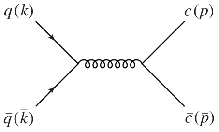
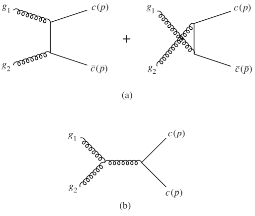
The leading-order Feynman diagrams for the production of a $c\bar{c}$ pair in color-octet states are presented in Figures 2 and 3. The diagram in Figure 2 ($q\bar{q}\to g\to c\bar{c}$) produces a $c\bar{c}(\underline{8},{}^{3}S_{1})$ state. The diagrams in Figure 3a (the gluon fusion process $gg\to c\bar{c}$) produce $c\bar{c}(\underline{8},{}^{1}S_{0})$, $c\bar{c}(\underline{8},{}^{3}S_{1})$ and $c\bar{c}(\underline{8},{}^{3}P_{J})$ states. The diagram in Figure 3b ($gg\to g\to c\bar{c}$) produces a $c\bar{c}(\underline{8},{}^{3}S_{1})$ state.

It is interesting to note that, at leading order in the ${\bf q}^{2}/m_{c}^{2}$ expansion, the amplitude for the production of $c\bar{c}(\underline{8},{}^{3}S_{1})$ from Figures 3a cancels against the amplitude for the same quantum number production in Figure 3b, so that the total production of $c\bar{c}(\underline{8},{}^{3}S_{1})$ from gluon-gluon collisions vanishes.

To determine the rough size of a term in the factorization formula, one attributes to it a power of $\alpha_{s}(m_{c})\approx 0.3$ for each vertex in the Feynman diagram, and the appropriate power of $v^{2}\approx 0.3$ according to its $v$-scaling. We summarize the $\alpha_{s}(m_{c})$ powers associated with the leading order subprocesses in Table II.

Once the most important terms in the factorization formula have been identified, one procedes to compute the short-distance coefficients $F_{n}$. This is done by matching perturbative full QCD and perturbative NRQCD calculations for the production rate of $c\bar{c}$ pairs with specific color and angular-momentum quantum numbers. These rates are expressed as an integral over relative momentum ${\bf q}$, with the integrand given as a Taylor expansion in ${\bf q}^{2}/m_{c}^{2}$

In the next sections, we calculate the production rates for the various important octet subprocesses contributing to hadronic $\psi$ production, and outline in detail the matching procedure.

III Production Rate for $q\bar{q}\to\psi$ Subprocess

We now calculate the leading-order contribution to the cross section for inclusive $\psi$ production from the color-octet subprocess $q\bar{q}\to\psi$. This is done in three steps. First we carry out a perturbative QCD calculation of the production rate for the process $q(k)\bar{q}(\bar{k})\to c(p)\bar{c}(\bar{p})$ with on-shell heavy quarks. The second step consists of calculating the production rate for the same process in NRQCD. The final step will be to determine the short-distance coefficient $F_{n}$ by matching the QCD and NRQCD calculations.

A Production rate in full QCD

In noncovariant conventions, the transition amplitude for the process $q(k)\bar{q}(\bar{k})\to c(p)\bar{c}(\bar{p})$, illustrated in FigureΒ 2, is given by

$${\cal T}\;=\;{g^{2}_{s}\over 4\sqrt{k_{0}\bar{k}_{0}p_{0}\bar{p}_{0}}}\;\bar{v}(\bar{k})\gamma^{\mu}T^{a}_{\bar{l}l}u(k)\;{1\over(p+\bar{p})^{2}}\;\bar{u}_{s}(p)\gamma_{\mu}T^{a}_{m\bar{m}}v_{\bar{s}}(\bar{p})\;,$$ (12)

where $l$, $\bar{l}$, $m$ and $\bar{m}$ are color indices and $s$ and $\bar{s}$ are heavy-quark spin indices. The matrices $T^{a}$ are normalized throughout so that $Tr[T^{a}T^{b}]=\delta^{ab}/2$. It is convenient to re-express the $c$ and $\bar{c}$ momentum in terms of ${\bf q}$ (the relative three-momentum of the quark and antiquark in the $c\bar{c}$ rest frame), and $P$ (the total four-momentum of the quark and anti-quark in the lab frame):

$\displaystyle p^{\mu}$ $\displaystyle=$ $\displaystyle{1\over 2}P^{\mu}\;+\;\Lambda^{\mu i}(P)q^{i},$ (13)
$\displaystyle\bar{p}^{\mu}$ $\displaystyle=$ $\displaystyle{1\over 2}P^{\mu}\;-\;\Lambda^{\mu i}(P)q^{i},$ (14)

where the Lorentz boost matrix $\Lambda^{\mu\nu}(P)$ is given by

$\displaystyle\Lambda^{0}_{j}$ $\displaystyle=$ $\displaystyle\frac{1}{2E_{q}}P^{j}$ (15)
$\displaystyle\Lambda^{i}_{j}$ $\displaystyle=$ $\displaystyle\delta^{ij}-\frac{P^{i}P^{j}}{{\bf P}^{2}}+\frac{P^{0}}{2E_{q}}\,\frac{P^{i}P^{j}}{{\bf P}^{2}}\;,$ (16)

with $E^{2}_{q}=m^{2}_{c}+{\bf q}^{2}$. The boost matrix has the following useful properties:

$\displaystyle\Lambda^{\mu}_{i}\Lambda^{\nu}_{j}\delta_{ij}$ $\displaystyle=$ $\displaystyle-g^{\mu\nu}+{P^{\mu}P^{\nu}\over P^{2}}$ (17)
$\displaystyle\Lambda^{\mu}_{i}\Lambda^{\nu}_{j}g_{\mu\nu}$ $\displaystyle=$ $\displaystyle-\delta_{ij}\;.$ (18)

The heavy quark Dirac bilinear $\bar{u}(p)\gamma^{\mu}v(\bar{p})$ appearing in Eq.Β (12) is now re-expressed in terms of ${\bf q}$, the Pauli two spinor $\xi$ and antispinor $\eta$, and the Pauli matrices $\sigma^{i}$Β [4]:

uΒ―s​(p)​γμ​vs¯​(pΒ―)=Ξ›jμ​(2​Eq​ξs†​σj​ηsΒ―βˆ’2Eq+mc​qj​ξs†​πͺβ‹…πˆβ€‹Ξ·sΒ―),subscript¯𝑒𝑠𝑝superscriptπ›Ύπœ‡subscript𝑣¯𝑠¯𝑝subscriptsuperscriptΞ›πœ‡π‘—2subscriptπΈπ‘žsubscriptsuperscriptπœ‰β€ π‘ superscriptπœŽπ‘—subscriptπœ‚Β―π‘ β‹…2subscriptπΈπ‘žsubscriptπ‘šπ‘superscriptπ‘žπ‘—subscriptsuperscriptπœ‰β€ π‘ πͺ𝝈subscriptπœ‚Β―π‘ \bar{u}_{s}(p)\gamma^{\mu}v_{\bar{s}}(\bar{p})=\Lambda^{\mu}_{j}\left(2E_{q}\;\xi^{\dagger}_{s}\sigma^{j}\eta_{\bar{s}}-{2\over E_{q}+m_{c}}\;q^{j}\xi^{\dagger}_{s}{\bf q}\cdot\mbox{\boldmath$\sigma$}\eta_{\bar{s}}\right)\;, (19)

where $\bar{u}_{s}(p)u_{s}(p)=2m_{c}$ and ΞΎs†​ξt=Ξ΄s​tsubscriptsuperscriptπœ‰β€ π‘ subscriptπœ‰π‘‘subscript𝛿𝑠𝑑\xi^{\dagger}_{s}\xi_{t}=\delta_{st}. The procedure of re-expressing the manifestly Lorentz-invariant Dirac bilinear current in terms of two-spinors can be called the β€œreduction of Dirac bilinears.” Applying the reduction to Eq.Β (12) we obtain

$\displaystyle{\cal T}$ $\displaystyle=$ $\displaystyle{g^{2}_{s}\over 2\sqrt{k_{0}\bar{k}_{0}(P^{2}_{0}-4({\bf\Lambda_{0}}\cdot{\bf q})^{2})}}\;\bar{v}(\bar{k})\gamma^{\mu}T^{a}_{\bar{l}l}u(k)\;{1\over 4E^{2}_{q}}$ (21)
Γ—Ξ›j​μ​(P)​(2​Eq​ξs†​σj​Tm​mΒ―a​ηsΒ―βˆ’2Eq+mc​qj​ξs†​πͺβ‹…πˆβ€‹Tm​mΒ―a​ηsΒ―).absentsubscriptΞ›π‘—πœ‡π‘ƒ2subscriptπΈπ‘žsubscriptsuperscriptπœ‰β€ π‘ superscriptπœŽπ‘—subscriptsuperscriptπ‘‡π‘Žπ‘šΒ―π‘šsubscriptπœ‚Β―π‘ β‹…2subscriptπΈπ‘žsubscriptπ‘šπ‘superscriptπ‘žπ‘—subscriptsuperscriptπœ‰β€ π‘ πͺ𝝈subscriptsuperscriptπ‘‡π‘Žπ‘šΒ―π‘šsubscriptπœ‚Β―π‘ \displaystyle\;\;\;\times\Lambda_{j\mu}(P)\left(2E_{q}\xi^{\dagger}_{s}\sigma^{j}T^{a}_{m\bar{m}}\eta_{\bar{s}}-{2\over E_{q}+m_{c}}q^{j}\xi^{\dagger}_{s}{\bf q}\cdot\mbox{\boldmath$\sigma$}T^{a}_{m\bar{m}}\eta_{\bar{s}}\right)\;.

(In the above context, the symbol $T^{a}_{m\bar{m}}$ represents a number, not a matrix; in our notation, the two-spinors $\xi$ and $\eta$ do not carry a color index and are not acted upon by the $T^{a}$. Our strategy of placing the factor $T^{a}_{m\bar{m}}$ between the two-spinors is designed to make the matching procedure more transparent.) The bilinear combination ΞΎs†​σj​ηsΒ―subscriptsuperscriptπœ‰β€ π‘ subscriptπœŽπ‘—subscriptπœ‚Β―π‘ \xi^{\dagger}_{s}\sigma_{j}\eta_{\bar{s}} corresponds to a ${}^{3}S_{1}$ spin configuration of the $c\bar{c}$ pair. Working to leading order in ${\bf q}$, we keep only the ${}^{3}S_{1}$ term:

𝒯=gs22​k0​kΒ―0​(P02βˆ’4​(πš²πŸŽβ‹…πͺ)2)​v¯​(kΒ―)​γμ​Tl¯​la​u​(k)​12​Eq​Λj​μ​(P)​ξs†​σj​Tm​mΒ―a​ηsΒ―.𝒯subscriptsuperscript𝑔2𝑠2subscriptπ‘˜0subscriptΒ―π‘˜0subscriptsuperscript𝑃204superscriptβ‹…subscript𝚲0πͺ2Β―π‘£Β―π‘˜superscriptπ›Ύπœ‡subscriptsuperscriptπ‘‡π‘ŽΒ―π‘™π‘™π‘’π‘˜12subscriptπΈπ‘žsubscriptΞ›π‘—πœ‡π‘ƒsubscriptsuperscriptπœ‰β€ π‘ superscriptπœŽπ‘—subscriptsuperscriptπ‘‡π‘Žπ‘šΒ―π‘šsubscriptπœ‚Β―π‘ {\cal T}\;=\;{g^{2}_{s}\over 2\sqrt{k_{0}\bar{k}_{0}(P^{2}_{0}-4({\bf\Lambda_{0}}\cdot{\bf q})^{2})}}\;\bar{v}(\bar{k})\gamma^{\mu}T^{a}_{\bar{l}l}u(k)\;{1\over 2E_{q}}\;\Lambda_{j\mu}(P)\;\xi^{\dagger}_{s}\sigma^{j}T^{a}_{m\bar{m}}\eta_{\bar{s}}\;. (22)

Anticipating that the probability of hadronization is negligible for $|{\bf q}|>\Lambda_{QCD}$, we need only derive the algebraic form of ${\cal T}$ for small ${\bf q}$, and therefore need only keep the first few terms in the Taylor expansion in ${\bf q}^{2}/m_{c}^{2}$:

π’―β‰ˆgs22​P0​k0​kΒ―0​v¯​(kΒ―)​γμ​Tl¯​la​u​(k)​12​mc​Λj​μ​ξs†​σj​Tm​mΒ―a​ηs¯​(1+a​πͺ2mc2+β‹―),𝒯subscriptsuperscript𝑔2𝑠2subscript𝑃0subscriptπ‘˜0subscriptΒ―π‘˜0Β―π‘£Β―π‘˜superscriptπ›Ύπœ‡subscriptsuperscriptπ‘‡π‘ŽΒ―π‘™π‘™π‘’π‘˜12subscriptπ‘šπ‘subscriptΞ›π‘—πœ‡subscriptsuperscriptπœ‰β€ π‘ superscriptπœŽπ‘—subscriptsuperscriptπ‘‡π‘Žπ‘šΒ―π‘šsubscriptπœ‚Β―π‘ 1π‘Žsuperscriptπͺ2superscriptsubscriptπ‘šπ‘2β‹―{\cal T}\;\approx\;{g^{2}_{s}\over 2P_{0}\sqrt{k_{0}\bar{k}_{0}}}\;\bar{v}(\bar{k})\gamma^{\mu}T^{a}_{\bar{l}l}u(k)\;{1\over 2m_{c}}\;\Lambda_{j\mu}\;\xi^{\dagger}_{s}\sigma^{j}T^{a}_{m\bar{m}}\eta_{\bar{s}}\left(1+a\frac{{\bf q}^{2}}{m_{c}^{2}}+\cdots\right)\;, (23)

where the constant $a$ β€” which we do not bother to calculate explicitly β€” is the coefficient of the second term in the Taylor series expansion in ${\bf q}^{2}/m_{c}^{2}$. It must be kept in mind that the factor appearing in brackets is not, at this point in the calculation, a rapidly converging series. Indeed, the upper bound on ${\bf q}$ is associated with the total momentum available in the experiment, and in general this can be much greater than $m_{c}$. However, for the purposes of matching in the factorization formalism, we treat ${\cal T}$ as an expansion in ${\bf q}^{2}/m_{c}^{2}$, and consider only the first few terms, the probability of hadronization being non-negligible only for small ${\bf q}$.

MultiplyingΒ (23) by its complex conjugate, summing over final colors and spins, and averaging over initial colors and spins, we obtain

|𝒯¯|2β‰ˆgs254​(2​mc)4​ξsβ€ β€‹πˆβ€‹Tm​mΒ―a​ηsΒ―β‹…Ξ·sΒ―β€ β€‹πˆβ€‹Tm¯​ma​ξs​(1+2​a​πͺ2mc2+β‹―),superscript¯𝒯2β‹…subscriptsuperscript𝑔2𝑠54superscript2subscriptπ‘šπ‘4subscriptsuperscriptπœ‰β€ π‘ πˆsubscriptsuperscriptπ‘‡π‘Žπ‘šΒ―π‘šsubscriptπœ‚Β―π‘ subscriptsuperscriptπœ‚β€ Β―π‘ πˆsubscriptsuperscriptπ‘‡π‘ŽΒ―π‘šπ‘šsubscriptπœ‰π‘ 12π‘Žsuperscriptπͺ2superscriptsubscriptπ‘šπ‘2β‹―|\bar{{\cal T}}|^{2}\;\approx\;{g^{2}_{s}\over 54(2m_{c})^{4}}\;\xi^{\dagger}_{s}\mbox{\boldmath$\sigma$}T^{a}_{m\bar{m}}\eta_{\bar{s}}\cdot\eta^{\dagger}_{\bar{s}}\mbox{\boldmath$\sigma$}T^{a}_{\bar{m}m}\xi_{s}\,\left(1+2a\frac{{\bf q}^{2}}{m_{c}^{2}}+\cdots\right)\;, (24)

where a sum over spins $s$ and $\bar{s}$ and color $m$ and $\bar{m}$ is assumed. Here we have made use of the fact that

βˆ‘s​sΒ―ΞΎs†​σi​ηs¯​ηs¯†​σj​ξs=Ξ΄i​j3β€‹βˆ‘s​sΒ―ΞΎsβ€ β€‹πˆβ€‹Ξ·sΒ―β‹…Ξ·sΒ―β€ β€‹πˆβ€‹ΞΎs.subscript𝑠¯𝑠subscriptsuperscriptπœ‰β€ π‘ superscriptπœŽπ‘–subscriptπœ‚Β―π‘ subscriptsuperscriptπœ‚β€ Β―π‘ superscriptπœŽπ‘—subscriptπœ‰π‘ superscript𝛿𝑖𝑗3subscript𝑠¯𝑠⋅subscriptsuperscriptπœ‰β€ π‘ πˆsubscriptπœ‚Β―π‘ subscriptsuperscriptπœ‚β€ Β―π‘ πˆsubscriptπœ‰π‘ \sum_{s\bar{s}}\;\xi^{\dagger}_{s}\sigma^{i}\eta_{\bar{s}}\;\;\eta^{\dagger}_{\bar{s}}\sigma^{j}\xi_{s}={\delta^{ij}\over 3}\;\sum_{s\bar{s}}\;\xi^{\dagger}_{s}\mbox{\boldmath$\sigma$}\eta_{\bar{s}}\cdot\eta^{\dagger}_{\bar{s}}\mbox{\boldmath$\sigma$}\xi_{s}\;. (25)

The expression for the cross section in terms of the transition amplitude squared is

$$\sigma={1\over F}\;\int{d^{3}{\bf p}\over(2\pi)^{3}}\int{d^{3}{\bf\bar{p}}\over(2\pi)^{3}}\;\;(2\pi)^{4}\delta^{4}(P-k-\bar{k})\;|\bar{{\cal T}}|^{2}\;,$$ (26)

where $F=2$ is the noncovariant flux. Changing variables from ${\bf p}$ and ${\bf\bar{p}}$ to ${\bf P}$ and ${\bf q}$, the above expression becomes

$\displaystyle\sigma$ $\displaystyle=$ $\displaystyle{1\over F}\;\int{d^{3}{\bf P}\over(2\pi)^{3}}\int{d^{3}{\bf q}\over(2\pi)^{3}}\;{P^{0}\over 2E_{q}}\;(2\pi)^{4}\delta^{4}(P-k-\bar{k})\;|\bar{{\cal T}}|^{2}\;$ (27)
$\displaystyle=$ $\displaystyle\pi\int{d^{3}{\bf q}\over(2\pi)^{3}}\;\;\delta(E_{f}-E_{i})\;|\bar{{\cal T}}|^{2}\;\left(1+a^{\prime}\frac{{\bf q}^{2}}{m_{c}^{2}}+\cdots\right).$ (28)

Inserting Eq.Β (24) into Eq.Β (28) we obtain the rate for on-shell $c\bar{c}$ production:

σ​(q​qΒ―β†’c​c¯​(8Β―,S13))=Ξ±s2​π354​mc4β€‹βˆ«d3​πͺ(2​π)3​δ​(Efβˆ’Ei)​ξsβ€ β€‹πˆβ€‹Tm​mΒ―a​ηs¯​ηsΒ―β€ β€‹πˆβ€‹Tm¯​ma​ξs​(1+a′′​πͺ2mc2+β‹―).πœŽβ†’π‘žΒ―π‘žπ‘Β―π‘Β―8superscriptsubscript𝑆13subscriptsuperscript𝛼2𝑠superscriptπœ‹354subscriptsuperscriptπ‘š4𝑐superscript𝑑3πͺsuperscript2πœ‹3𝛿subscript𝐸𝑓subscript𝐸𝑖subscriptsuperscriptπœ‰β€ π‘ πˆsubscriptsuperscriptπ‘‡π‘Žπ‘šΒ―π‘šsubscriptπœ‚Β―π‘ subscriptsuperscriptπœ‚β€ Β―π‘ πˆsubscriptsuperscriptπ‘‡π‘ŽΒ―π‘šπ‘šsubscriptπœ‰π‘ 1superscriptπ‘Žβ€²β€²superscriptπͺ2superscriptsubscriptπ‘šπ‘2β‹―\sigma(q\bar{q}\to c\bar{c}(\underline{8},{}^{3}S_{1}))={\alpha^{2}_{s}\pi^{3}\over 54m^{4}_{c}}\;\int{d^{3}{\bf q}\over(2\pi)^{3}}\;\delta(E_{f}-E_{i})\;\xi^{\dagger}_{s}\mbox{\boldmath$\sigma$}T^{a}_{m\bar{m}}\eta_{\bar{s}}\;\;\eta^{\dagger}_{\bar{s}}\mbox{\boldmath$\sigma$}T^{a}_{\bar{m}m}\xi_{s}\;\left(1+a^{\prime\prime}\frac{{\bf q}^{2}}{m_{c}^{2}}+\cdots\right). (29)

B Production rate in NRQCD

The next step is to calculate the production rate for the process $q\bar{q}\to c\bar{c}(\underline{8},{}^{3}S_{1})$ in perturbative NRQCD. The first two terms are

$$\sigma(q\bar{q}\to c\bar{c}(\underline{8},{}^{3}S_{1}))=\int\frac{d^{3}{\bf q}}{(2\pi)^{3}}\left(\;\;\frac{F_{8}({}^{3}S_{1})}{m_{c}^{2}}\;\;\langle 0|{\cal O}^{c\bar{c}(q)}_{8}({}^{3}S_{1})|0\rangle\;+\;\frac{G_{8}({}^{3}S_{1})}{m_{c}^{4}}\;\;\langle 0|{\cal P}^{c\bar{c}(q)}_{8}({}^{3}S_{1})|0\rangle+\cdots\right)\;,$$ (30)

where $F_{8}({}^{3}S_{1})$ and $G_{8}({}^{3}S_{1})$ are specific cases of the short-distance coefficients $F_{n}$, and where

$\displaystyle\langle 0|{\cal O}^{c\bar{c}(q)}_{8}({}^{3}S_{1})|0\rangle$ $\displaystyle=$ βˆ‘s​s¯​m​m¯⟨0|χ†​σi​Taβ€‹Οˆ|c​(s,m,πͺ)​c¯​(sΒ―,mΒ―,βˆ’πͺ)⟩subscriptπ‘ Β―π‘ π‘šΒ―π‘šquantum-operator-product0superscriptπœ’β€ superscriptπœŽπ‘–superscriptπ‘‡π‘Žπœ“π‘π‘ π‘šπͺΒ―π‘Β―π‘ Β―π‘šπͺ\displaystyle\sum_{s\bar{s}m\bar{m}}\langle 0|\chi^{\dagger}\sigma^{i}T^{a}\psi|c(s,m,{\bf q})\bar{c}(\bar{s},\bar{m},-{\bf q})\rangle (32)
⟨c​(s,m,πͺ)​c¯​(sΒ―,mΒ―,βˆ’πͺ)|Οˆβ€ β€‹Οƒi​Ta​χ|0⟩quantum-operator-productπ‘π‘ π‘šπͺΒ―π‘Β―π‘ Β―π‘šπͺsuperscriptπœ“β€ superscriptπœŽπ‘–superscriptπ‘‡π‘Žπœ’0\displaystyle\qquad\langle c(s,m,{\bf q})\bar{c}(\bar{s},\bar{m},-{\bf q})|\psi^{\dagger}\sigma^{i}T^{a}\chi|0\rangle
$\displaystyle\langle 0|{\cal P}^{c\bar{c}(q)}_{8}({}^{3}S_{1})|0\rangle$ $\displaystyle=$ $\displaystyle\frac{1}{2}\sum_{s\bar{s}m\bar{m}}\langle 0|\chi^{\dagger}\sigma^{i}T^{a}\left(-\frac{i}{2}\stackrel{{\scriptstyle\leftrightarrow}}{{{\bf D}}}\right)^{2}\psi|c(s,m,{\bf q})\bar{c}(\bar{s},\bar{m},-{\bf q})\rangle$ (34)
⟨c​(s,m,πͺ)​c¯​(sΒ―,mΒ―,βˆ’πͺ)|Οˆβ€ β€‹Οƒi​Ta​χ|0⟩quantum-operator-productπ‘π‘ π‘šπͺΒ―π‘Β―π‘ Β―π‘šπͺsuperscriptπœ“β€ superscriptπœŽπ‘–superscriptπ‘‡π‘Žπœ’0\displaystyle\qquad\langle c(s,m,{\bf q})\bar{c}(\bar{s},\bar{m},-{\bf q})|\psi^{\dagger}\sigma^{i}T^{a}\chi|0\rangle
$\displaystyle+$ 12β€‹βˆ‘s​s¯​m​m¯⟨0|χ†​σi​Taβ€‹Οˆ|c​(s,m,πͺ)​c¯​(sΒ―,mΒ―,βˆ’πͺ)⟩12subscriptπ‘ Β―π‘ π‘šΒ―π‘šquantum-operator-product0superscriptπœ’β€ superscriptπœŽπ‘–superscriptπ‘‡π‘Žπœ“π‘π‘ π‘šπͺΒ―π‘Β―π‘ Β―π‘šπͺ\displaystyle\frac{1}{2}\sum_{s\bar{s}m\bar{m}}\langle 0|\chi^{\dagger}\sigma^{i}T^{a}\psi|c(s,m,{\bf q})\bar{c}(\bar{s},\bar{m},-{\bf q})\rangle (36)
⟨c(s,m,πͺ)cΒ―(sΒ―,mΒ―,βˆ’πͺ)|Οˆβ€ ΟƒiTa(βˆ’i2𝐃↔)2Ο‡|0⟩.\displaystyle\qquad\langle c(s,m,{\bf q})\bar{c}(\bar{s},\bar{m},-{\bf q})|\psi^{\dagger}\sigma^{i}T^{a}\left(-\frac{i}{2}\stackrel{{\scriptstyle\leftrightarrow}}{{{\bf D}}}\right)^{2}\chi|0\rangle\;.

Our task here is to derive explicit expressions for the $c\bar{c}(q)$ matrix elements in Eqs.Β (32) and (36). For practical reasons, it is worthwhile to quickly note one possible set of conventions for these calculations. Let us define the single-particle annihilation and creation operators to obey the anticommutation relation [a​(s,i,πͺ),a†​(t,j,𝐩)]=(2​π)3​δ​(πͺβˆ’π©)​δs​t​δi​jπ‘Žπ‘ π‘–πͺsuperscriptπ‘Žβ€ π‘‘π‘—π©superscript2πœ‹3𝛿πͺ𝐩superscript𝛿𝑠𝑑superscript𝛿𝑖𝑗[a(s,i,{\bf q}),a^{\dagger}(t,j,{\bf p})]=(2\pi)^{3}\delta({\bf q}-{\bf p})\delta^{st}\delta^{ij}. The annihilation operator acts according to a​(s,i,πͺ)​|c​(t,j,𝐩)⟩=(2​π)3​δ​(πͺβˆ’π©)​δs​t​δi​j​|0βŸ©π‘Žπ‘ π‘–πͺket𝑐𝑑𝑗𝐩superscript2πœ‹3𝛿πͺ𝐩superscript𝛿𝑠𝑑superscript𝛿𝑖𝑗ket0a(s,i,{\bf q})|c(t,j,{\bf p})\rangle=(2\pi)^{3}\delta({\bf q}-{\bf p})\delta^{st}\delta^{ij}|0\rangle, and the creation operator according to a†​(t,j,πͺ)​|0⟩=|c​(t,j,πͺ)⟩superscriptπ‘Žβ€ π‘‘π‘—πͺket0ket𝑐𝑑𝑗πͺa^{\dagger}(t,j,{\bf q})|0\rangle=|c(t,j,{\bf q})\rangle. Single particle states are normalized so that $\langle c(s,i,{\bf q})|c(t,j,{\bf p})\rangle=(2\pi)^{3}\delta({\bf q}-{\bf p})\delta^{st}\delta^{ij}$. Then, conceiving of the field operators $\psi$ and $\chi$ as color-triplet vectors, we write their Fourier decompositions as

$\displaystyle\psi_{m}(x)$ $\displaystyle=$ βˆ‘s∫d3​p(2​π)3​a​(s,m,𝐩)​ξs​eβˆ’i​pβ‹…xsubscript𝑠superscript𝑑3𝑝superscript2πœ‹3π‘Žπ‘ π‘šπ©subscriptπœ‰π‘ superscript𝑒⋅𝑖𝑝π‘₯\displaystyle\sum_{s}\int{d^{3}p\over(2\pi)^{3}}a(s,m,{\bf p})\xi_{s}e^{-ip\cdot x} (37)
Ο‡m¯†​(x)subscriptsuperscriptπœ’β€ Β―π‘šπ‘₯\displaystyle\chi^{\dagger}_{\bar{m}}(x) $\displaystyle=$ βˆ‘s¯∫d3​p(2​π)3​b​(sΒ―,mΒ―,𝐩)​ηs¯†​eβˆ’i​pβ‹…x,subscript¯𝑠superscript𝑑3𝑝superscript2πœ‹3π‘Β―π‘ Β―π‘šπ©subscriptsuperscriptπœ‚β€ Β―π‘ superscript𝑒⋅𝑖𝑝π‘₯\displaystyle\sum_{\bar{s}}\int{d^{3}p\over(2\pi)^{3}}b(\bar{s},\bar{m},{\bf p})\eta^{\dagger}_{\bar{s}}e^{-ip\cdot x}\;, (38)

where ΞΎssubscriptπœ‰π‘ \xi_{s} and Ξ·s¯†subscriptsuperscriptπœ‚β€ Β―π‘ \eta^{\dagger}_{\bar{s}} are the two-spinors.

Using the conventions outlined in the preceding paragraph, we derive explicit expressions for the right-hand-side of Eq.Β (30), obtaining

σ​(q​qΒ―β†’c​c¯​(8Β―,S13))=∫d3​πͺ(2​π)3​(F8​(S13)mc2+G8​(S13)mc2​πͺ2mc2+β‹―)​ξsβ€ β€‹πˆβ€‹Tm​mΒ―a​ηs¯​ηsΒ―β€ β€‹πˆβ€‹Tm¯​ma​ξs.πœŽβ†’π‘žΒ―π‘žπ‘Β―π‘Β―8superscriptsubscript𝑆13superscript𝑑3πͺsuperscript2πœ‹3subscript𝐹8superscriptsubscript𝑆13superscriptsubscriptπ‘šπ‘2subscript𝐺8superscriptsubscript𝑆13superscriptsubscriptπ‘šπ‘2superscriptπͺ2superscriptsubscriptπ‘šπ‘2β‹―subscriptsuperscriptπœ‰β€ π‘ πˆsubscriptsuperscriptπ‘‡π‘Žπ‘šΒ―π‘šsubscriptπœ‚Β―π‘ subscriptsuperscriptπœ‚β€ Β―π‘ πˆsubscriptsuperscriptπ‘‡π‘ŽΒ―π‘šπ‘šsubscriptπœ‰π‘ \sigma(q\bar{q}\to c\bar{c}(\underline{8},{}^{3}S_{1}))=\int\frac{d^{3}{\bf q}}{(2\pi)^{3}}\left(\;\;\frac{F_{8}({}^{3}S_{1})}{m_{c}^{2}}\;+\;\frac{G_{8}({}^{3}S_{1})}{m_{c}^{2}}\;\frac{{\bf q}^{2}}{m_{c}^{2}}+\cdots\right)\;\xi^{\dagger}_{s}\mbox{\boldmath$\sigma$}T^{a}_{m\bar{m}}\eta_{\bar{s}}\;\;\eta^{\dagger}_{\bar{s}}\mbox{\boldmath$\sigma$}T^{a}_{\bar{m}m}\xi_{s}\;. (39)

C Matching

Finally we determine the short-distance coefficient by matching the perturbative QCD result Eq.Β (29) to the perturbative NRQCD result Eq.Β (39)

$\displaystyle F_{8}({}^{3}S_{1})$ $\displaystyle=$ 2​αs2​π327​mc​δ​(sβˆ’4​mc2)2subscriptsuperscript𝛼2𝑠superscriptπœ‹327subscriptπ‘šπ‘π›Ώπ‘ 4subscriptsuperscriptπ‘š2𝑐\displaystyle{2\alpha^{2}_{s}\pi^{3}\over 27m_{c}}\;\delta(s-4m^{2}_{c}) (40)
$\displaystyle G_{8}({}^{3}S_{1})$ $\displaystyle=$ 2​a′′​αs2​π327​mc​δ​(sβˆ’4​mc2).2superscriptπ‘Žβ€²β€²subscriptsuperscript𝛼2𝑠superscriptπœ‹327subscriptπ‘šπ‘π›Ώπ‘ 4subscriptsuperscriptπ‘š2𝑐\displaystyle{2a^{\prime\prime}\alpha^{2}_{s}\pi^{3}\over 27m_{c}}\;\delta(s-4m^{2}_{c})\;. (41)

The matching procedure for on-shell scattering fixes the short-distance coefficient in the non-relativistic effective theory. However, these same coefficients apply to the calculation of the production of bound quarkonium states. This is because the non-perturbative effects that will bind the $c$ and $\bar{c}$ into a charmonium meson take place over much longer distances than the separation $1/m_{c}$ associated with the formation of the $c\bar{c}$ pair. Thus, although the short-distance coefficient has been determined using a perturbative calculation of the production of free quarks and antiquarks, the same short-distance coefficient applies to the formation of a $c\bar{c}$ pair in a charmonium state. The nonperturbative effects involved in the formation of the boundstate are described by the matrix elements. Therefore, the inclusive cross section for $q\bar{q}\to\psi$ via the color-octet mechanism is, to leading order in $v^{2}$,

$\displaystyle\sigma(q\bar{q}\to\psi)$ $\displaystyle=$ $\displaystyle\frac{F_{8}({}^{3}S_{1})}{m_{c}^{2}}\langle 0|{\cal O}_{8}^{\psi}({}^{3}S_{1})|0\rangle$ (42)
$\displaystyle=$ $\displaystyle{2\alpha^{2}_{s}\pi^{3}\over 27m^{3}_{c}}\;\delta(s-4m^{2}_{c})\langle 0|{\cal O}^{\psi}_{8}({}^{3}S_{1})|0\rangle\;.$ (43)

This procedure, which involves the determination of the $F_{n}$ for the production of on-shell heavy quarks, correctly takes into account the effects of binding energy, as can be verified by explicit calculations in NRQEDΒ [5].

IV Cross section for $gg\to\psi$ subprocess

Next we turn our attention to the process $g(g_{1})g(g_{2})\to c(p)\bar{c}(\bar{p})$ which, at leading order in $\alpha_{s}$, proceeds through the Feynman diagrams in FigureΒ 3. To determine the short-distance coefficients we follow a sequence of steps analogous to that outlined in the previous section. At this point we will abandon or habit of writing heavy quark spin and color indices explicitly.

The transition amplitude calculated from the diagrams in FigureΒ 3a is

$\displaystyle{\cal T}(gg\to c\bar{c})={-g^{2}_{s}\over 4\sqrt{g_{10}g_{20}p_{0}\bar{p}_{0}}}\;\epsilon_{\mu}(g_{1})\epsilon_{\nu}(g_{2})$ (45)
$\displaystyle\;\;\;\bar{u}(p)\left[T^{a}T^{b}{\gamma^{\mu}(\not\!p-\not\!g_{1}+m_{c})\gamma^{\nu}\over 2p\cdot g_{1}}\right.+T^{b}T^{a}{\gamma^{\nu}(-\not\!\bar{p}+\not\!g_{1}+m_{c})\gamma^{\mu}\over 2\bar{p}\cdot g_{1}}\left.\right]v(\bar{p})\;.$

The product of color matrices in Eq.Β (45) can be rewritten as

$$T^{a}T^{b}={1\over 6}\delta^{ab}+{1\over 2}(d^{abc}+if^{abc})T^{c},$$ (46)

where $d^{abc}$ is a symmetric tensor and $f^{abc}$ is an antisymmetric tensor. Since we wish to determine the short-distance coefficient for color-octet production, we will discard the $\delta^{ab}/6$ term of Eq.Β (46). Then, using the Dirac equation, Eq.Β (45) can be transformed into

$\displaystyle{\cal T}(gg\to c\bar{c})$ $\displaystyle=$ $\displaystyle{g^{2}_{s}\over 16E_{q}^{2}\sqrt{g_{10}g_{20}p_{0}\bar{p}_{0}}}\left[1-{(g_{1}\cdot\Lambda q)^{2}\over E_{q}^{4}}\right]^{-1}\;\epsilon_{\mu}(g_{1})\epsilon_{\nu}(g_{2})$ (48)
$\displaystyle\;\;\;\;\bar{u}(p)\Bigg{\{}d^{abc}T^{c}\left[{\cal A}^{\mu\nu}-{g_{1}\cdot\Lambda q\over E_{q}^{2}}{\cal B}^{\mu\nu}\right]\;+\;if^{abc}T^{c}\left[{\cal B}^{\mu\nu}-{g_{1}\cdot\Lambda q\over E_{q}^{2}}{\cal A}^{\mu\nu}\right]\Bigg{\}}v(\bar{p})\;,$

where

$${\cal A}^{\mu\nu}=i\epsilon^{\mu\nu\alpha\beta}(g_{1}-g_{2})_{\alpha}\gamma_{\beta}\gamma_{5}\;+\;2\left[(\Lambda q)^{\mu}\gamma^{\nu}+(\Lambda q)^{\nu}\gamma^{\mu}\right]\;,$$ (50)

and

$${\cal B}^{\mu\nu}=2g^{\mu}_{2}\gamma^{\nu}-2g^{\nu}_{1}\gamma^{\mu}+g^{\mu\nu}(\not\!g_{1}-\not\!g_{2})\;.$$ (51)

We reduce the Dirac bilinears using Eq.Β (19) and

u¯​(p)​γμ​γ5​v​(pΒ―)=mcEq​PΞΌβ€‹ΞΎβ€ β€‹Ξ·βˆ’2​i​Λjμ​ξ†​(πͺΓ—πˆ)j​η.¯𝑒𝑝superscriptπ›Ύπœ‡subscript𝛾5𝑣¯𝑝subscriptπ‘šπ‘subscriptπΈπ‘žsuperscriptπ‘ƒπœ‡superscriptπœ‰β€ πœ‚2𝑖subscriptsuperscriptΞ›πœ‡π‘—superscriptπœ‰β€ superscriptπͺπˆπ‘—πœ‚\bar{u}(p)\gamma^{\mu}\gamma_{5}v(\bar{p})={m_{c}\over E_{q}}P^{\mu}\;\xi^{\dagger}\eta-2i\Lambda^{\mu}_{j}\xi^{\dagger}({\bf q}\times\mbox{\boldmath$\sigma$})^{j}\eta\;. (52)

Keeping only terms of leading order in ${\bf q}$, the resulting amplitude may be expressed in the form

$${\cal T}(gg\to c\bar{c})\approx{\cal T}_{CS}(gg\to c\bar{c})+{\cal T}_{CAS}(gg\to c\bar{c})\;,$$ (53)

where ${\cal T}_{CS}$ is the color symmetric piece

$\displaystyle{\cal T}_{CS}(gg\to c\bar{c})$ $\displaystyle=$ $\displaystyle d^{abc}{g^{2}_{s}\over(2m_{c})^{4}}\epsilon_{\mu}(g_{1})\epsilon_{\nu}(g_{2})\Bigg{\{}i\epsilon^{\mu\nu\alpha\beta}(g_{1}-g_{2})_{\alpha}P_{\beta}\;\xi^{\dagger}T^{c}\eta$ (54)
$\displaystyle+$ $\displaystyle\left[2\epsilon^{\mu\nu\alpha\beta}(g_{1}-g_{2})_{\alpha}\epsilon^{ijk}\Lambda^{k}_{\beta}+4m_{c}(\Lambda^{\mu}_{i}\Lambda^{\nu}_{j}+\Lambda^{\nu}_{i}\Lambda^{\mu}_{j})\right.$ (55)
$\displaystyle-{2\over m_{c}}(g_{1}\cdot\Lambda)_{i}(2g^{\mu}_{2}\Lambda^{\nu}_{j}$ $\displaystyle-$ $\displaystyle 2g^{\nu}_{1}\Lambda^{\mu}_{j}+g^{\mu\nu}(g_{1}-g_{2})\cdot\Lambda_{j})\left.\right]q^{i}\xi^{\dagger}\sigma^{j}T^{c}\eta\Bigg{\}}\;+\cdots\;,$ (56)

and where ${\cal T}_{CAS}$ is the color antisymmetric part

$\displaystyle{\cal T}_{CAS}(gg\to c\bar{c})$ $\displaystyle=$ $\displaystyle if^{abc}{g^{2}_{s}\over(2m_{c})^{3}}\epsilon_{\mu}(g_{1})\epsilon_{\nu}(g_{2})$ (58)
[2​g2μ​ΛjΞ½βˆ’2​g1ν​ΛjΞΌ+gμ​ν​(g1βˆ’g2)β‹…Ξ›j]​ξ†​σj​Tc​η+β‹―.delimited-[]2subscriptsuperscriptπ‘”πœ‡2subscriptsuperscriptΞ›πœˆπ‘—2subscriptsuperscriptπ‘”πœˆ1subscriptsuperscriptΞ›πœ‡π‘—β‹…superscriptπ‘”πœ‡πœˆsubscript𝑔1subscript𝑔2subscriptΛ𝑗superscriptπœ‰β€ superscriptπœŽπ‘—superscriptπ‘‡π‘πœ‚β‹―\displaystyle\qquad\left[2g^{\mu}_{2}\Lambda^{\nu}_{j}-2g^{\nu}_{1}\Lambda^{\mu}_{j}+g^{\mu\nu}(g_{1}-g_{2})\cdot\Lambda_{j}\right]\xi^{\dagger}\sigma^{j}T^{c}\eta\;+\cdots\;.

The dots $\cdots$ are included as a reminder that we are writing only the first term in the infinite and non-convergent series in ${\bf q}^{2}/m_{c}^{2}$. This is justified since the factorization formalism requires only that we know the algebraic form of ${\cal T}$ for small ${\bf q}$.

We note that at leading order in the non-relativistic expansion, the amplitude for producing $c\bar{c}(\underline{8},{}^{3}S_{1}))$ in Figure 3b, Eq.Β (58) cancels against the contribution from the gluon-fusion graphs in Figure 3a, leaving only the pieces in Eq.Β (56).

We now turn to the task of isolating the terms in Eq.Β (56) that contribute to the production of $c\bar{c}$ pairs in the states $\underline{8},{}^{1}S_{0}$, $\underline{8},{}^{3}P_{0}$ and $\underline{8},{}^{3}P_{2}$. Beginning with $\underline{8},{}^{1}S_{0}$, we note that terms associated with the angular-momentum quantum numbers ${}^{1}S_{0}$ will have Pauli-spinor bilinears of the form ξ†​ηsuperscriptπœ‰β€ πœ‚\xi^{\dagger}\eta, πͺ2​ξ†​ηsuperscriptπͺ2superscriptπœ‰β€ πœ‚{\bf q}^{2}\xi^{\dagger}\eta, etc. It is an easy matter to pick out the ${}^{1}S_{0}$ pieces in Eq.Β (56):

𝒯​(g​gβ†’c​c¯​(8Β―,S01))=i​da​b​c​gs2(2​mc)4​ϡμ​(g1)​ϡν​(g2)​ϡμ​ν​α​β​(g1βˆ’g2)α​Pβ​ξ†​Tc​η​(1+β‹―).𝒯→𝑔𝑔𝑐¯𝑐¯8superscriptsubscript𝑆01𝑖superscriptπ‘‘π‘Žπ‘π‘subscriptsuperscript𝑔2𝑠superscript2subscriptπ‘šπ‘4subscriptitalic-Ο΅πœ‡subscript𝑔1subscriptitalic-ϡ𝜈subscript𝑔2superscriptitalic-Ο΅πœ‡πœˆπ›Όπ›½subscriptsubscript𝑔1subscript𝑔2𝛼subscript𝑃𝛽superscriptπœ‰β€ superscriptπ‘‡π‘πœ‚1β‹―{\cal T}(gg\to c\bar{c}(\underline{8},{}^{1}S_{0}))=id^{abc}{g^{2}_{s}\over(2m_{c})^{4}}\;\epsilon_{\mu}(g_{1})\epsilon_{\nu}(g_{2})\;\epsilon^{\mu\nu\alpha\beta}(g_{1}-g_{2})_{\alpha}P_{\beta}\;\;\xi^{\dagger}T^{c}\eta\;\;(1+\cdots)\;. (59)

Squaring Eq.Β (59), and performing the sum-average over spins and colors, we obtain

|𝒯¯​(g​gβ†’c​c¯​(8Β―,S01))|2=5​gs4384​(2​mc)4​ξ†​Tc​η​η†​Tc​ξ​(1+β‹―).superscript¯𝒯→𝑔𝑔𝑐¯𝑐¯8superscriptsubscript𝑆0125subscriptsuperscript𝑔4𝑠384superscript2subscriptπ‘šπ‘4superscriptπœ‰β€ superscriptπ‘‡π‘πœ‚superscriptπœ‚β€ superscriptπ‘‡π‘πœ‰1β‹―|\bar{{\cal T}}(gg\to c\bar{c}(\underline{8},{}^{1}S_{0}))|^{2}={5g^{4}_{s}\over 384(2m_{c})^{4}}\;\;\xi^{\dagger}T^{c}\eta\;\;\eta^{\dagger}T^{c}\xi\;\;(1+\cdots)\;. (60)

Inserting this into the expression for the cross section given in Eq.Β (28) we obtain

σ​(g​gβ†’c​c¯​(8Β―,S01))β‰ˆ5​π3​αs23β‹…128​mc4β€‹βˆ«d3​πͺ(2​π)3​δ​(Efβˆ’Ei)​ξ†​Tc​η​η†​Tc​ξ​(1+β‹―),πœŽβ†’π‘”π‘”π‘Β―π‘Β―8superscriptsubscript𝑆015superscriptπœ‹3subscriptsuperscript𝛼2𝑠⋅3128superscriptsubscriptπ‘šπ‘4superscript𝑑3πͺsuperscript2πœ‹3𝛿subscript𝐸𝑓subscript𝐸𝑖superscriptπœ‰β€ superscriptπ‘‡π‘πœ‚superscriptπœ‚β€ superscriptπ‘‡π‘πœ‰1β‹―\sigma(gg\to c\bar{c}(\underline{8},{}^{1}S_{0}))\approx{5\pi^{3}\alpha^{2}_{s}\over 3\cdot 128\,m_{c}^{4}}\;\int{d^{3}{\bf q}\over(2\pi)^{3}}\;\delta(E_{f}-E_{i})\;\;\xi^{\dagger}T^{c}\eta\;\;\eta^{\dagger}T^{c}\xi\;\;(1+\cdots)\;, (61)

which is the result in full QCD for the production rate of an on-shell $c\bar{c}(\underline{8},{}^{1}S_{0})$.

The next step consists of calculating the same production rate in perturbative NRQCD. This is given by

$\displaystyle\sigma(gg\to c\bar{c}(\underline{8},{}^{1}S_{0}))$ $\displaystyle=$ $\displaystyle\int\frac{d^{3}{\bf q}}{(2\pi)^{3}}\;\frac{F_{8}({}^{1}S_{0})}{m_{c}^{2}}\;\langle 0|{\cal O}^{c\bar{c}(q)}_{8}({}^{1}S_{0})|0\rangle+\cdots$ (62)
$\displaystyle=$ ∫d3​πͺ(2​π)3​F8​(S01)mc2β€‹βˆ‘s​s¯​m​m¯⟨0|χ†​Taβ€‹Οˆ|c​(s,m,πͺ)​c¯​(sΒ―,mΒ―,βˆ’πͺ)⟩superscript𝑑3πͺsuperscript2πœ‹3subscript𝐹8superscriptsubscript𝑆01superscriptsubscriptπ‘šπ‘2subscriptπ‘ Β―π‘ π‘šΒ―π‘šquantum-operator-product0superscriptπœ’β€ superscriptπ‘‡π‘Žπœ“π‘π‘ π‘šπͺΒ―π‘Β―π‘ Β―π‘šπͺ\displaystyle\int\frac{d^{3}{\bf q}}{(2\pi)^{3}}\;\frac{F_{8}({}^{1}S_{0})}{m_{c}^{2}}\;\sum_{s\bar{s}m\bar{m}}\langle 0|\chi^{\dagger}T^{a}\psi|c(s,m,{\bf q})\bar{c}(\bar{s},\bar{m},-{\bf q})\rangle (64)
⟨c​(s,m,πͺ)​c¯​(sΒ―,mΒ―,βˆ’πͺ)|Οˆβ€ β€‹Ta​χ|0⟩+β‹―quantum-operator-productπ‘π‘ π‘šπͺΒ―π‘Β―π‘ Β―π‘šπͺsuperscriptπœ“β€ superscriptπ‘‡π‘Žπœ’0β‹―\displaystyle\qquad\langle c(s,m,{\bf q})\bar{c}(\bar{s},\bar{m},-{\bf q})|\psi^{\dagger}T^{a}\chi|0\rangle+\cdots
$\displaystyle=$ ∫d3​πͺ(2​π)3​F8​(S01)mc2​ξ†​Tc​η​η†​Tc​ξ+β‹―.superscript𝑑3πͺsuperscript2πœ‹3subscript𝐹8superscriptsubscript𝑆01superscriptsubscriptπ‘šπ‘2superscriptπœ‰β€ superscriptπ‘‡π‘πœ‚superscriptπœ‚β€ superscriptπ‘‡π‘πœ‰β‹―\displaystyle\int{d^{3}{\bf q}\over(2\pi)^{3}}\;\frac{F_{8}({}^{1}S_{0})}{m_{c}^{2}}\;\;\xi^{\dagger}T^{c}\eta\;\;\eta^{\dagger}T^{c}\xi\;+\cdots\;. (65)

Matching the result from full QCD in Eq.Β (61) to that from NRQCD in Eq.Β (65), we obtain

F8​(S01)=5​π3​αs296​mc​δ​(sβˆ’4​mc2),subscript𝐹8superscriptsubscript𝑆015superscriptπœ‹3superscriptsubscript𝛼𝑠296subscriptπ‘šπ‘π›Ώπ‘ 4superscriptsubscriptπ‘šπ‘2F_{8}({}^{1}S_{0})=\frac{5\pi^{3}\alpha_{s}^{2}}{96m_{c}}\delta(s-4m_{c}^{2})\;, (66)

from which we conclude that

$\displaystyle\sigma(gg\to\psi+X)$ $\displaystyle=$ $\displaystyle\frac{F_{8}({}^{1}S_{0})}{m_{c}^{2}}\langle 0|{\cal O}^{\psi}_{8}({}^{1}S_{0})|0\rangle$ (67)
$\displaystyle=$ $\displaystyle{5\pi^{3}\alpha^{2}_{s}\over 96m_{c}^{3}}\;\delta(s-4m^{2}_{c})\;\langle 0|{\cal O}^{\psi}_{8}({}^{1}S_{0})|0\rangle\;.$ (68)

Next we isolate the individual $P$-wave contributions. This can be accomplished by first noting that any direct product of cartesian vectors may be written as

$$a^{i}b^{j}={1\over 3}\delta^{ij}\;{\bf a}\cdot{\bf b}+{1\over 2}\epsilon^{ijk}({\bf a}\times{\bf b})^{k}+a^{[i}b^{j]}\;,$$ (69)

where $a^{[i}b^{j]}=(a^{i}b^{j}+a^{j}b^{i})/2-{\bf a}\cdot{\bf b}\;\delta^{ij}/3$. Thus we are able to decompose the factor qi​ξ†​σj​ηsuperscriptπ‘žπ‘–superscriptπœ‰β€ superscriptπœŽπ‘—πœ‚q^{i}\xi^{\dagger}\sigma^{j}\eta appearing in the second term on the right-hand-side of Eq.Β (56) into a scalar component that is identified with the ${}^{3}P_{0}$ state, a vector component identified with the ${}^{3}P_{1}$ state, and a symmetric-traceless tensor component identified with the ${}^{3}P_{2}$ state. We wish to emphasize that the procedure of decomposing the amplitude into seperate angular-momentum configurations, ${}^{1}S_{0}$, ${}^{3}S_{1}$, ${}^{3}P_{0}$, ${}^{3}P_{1}$, etc. can be carried out to any order in the ${\bf q}^{2}/m^{2}_{c}$ expansion. It is always possible to decompose the amplitude for the production of a heavy quark-antiquark pair into pieces of the form

$\displaystyle{\cal T}(i\rightarrow c\bar{c}({}^{1}S_{0}))$ $\displaystyle=$ A​ξ†​η​(1+a​πͺ2mc2+β‹―)𝐴superscriptπœ‰β€ πœ‚1π‘Žsuperscriptπͺ2superscriptsubscriptπ‘šπ‘2β‹―\displaystyle A\;\xi^{\dagger}\eta\left(1+a\frac{{\bf q}^{2}}{m_{c}^{2}}+\cdots\right) (70)
$\displaystyle{\cal T}(i\rightarrow c\bar{c}({}^{3}S_{1}))$ $\displaystyle=$ Ai​ξ†​σi​η​(1+a​πͺ2mc2+β‹―)superscript𝐴𝑖superscriptπœ‰β€ superscriptπœŽπ‘–πœ‚1π‘Žsuperscriptπͺ2superscriptsubscriptπ‘šπ‘2β‹―\displaystyle A^{i}\;\xi^{\dagger}\sigma^{i}\eta\left(1+a\frac{{\bf q}^{2}}{m_{c}^{2}}+\cdots\right) (71)
$\displaystyle{\cal T}(i\rightarrow c\bar{c}({}^{1}P_{1}))$ $\displaystyle=$ Ai​ξ†​qi​η​(1+a​πͺ2mc2+β‹―)superscript𝐴𝑖superscriptπœ‰β€ superscriptπ‘žπ‘–πœ‚1π‘Žsuperscriptπͺ2superscriptsubscriptπ‘šπ‘2β‹―\displaystyle A^{i}\;\xi^{\dagger}q^{i}\eta\left(1+a\frac{{\bf q}^{2}}{m_{c}^{2}}+\cdots\right) (72)
𝒯​(iβ†’c​c¯​(P03))𝒯→𝑖𝑐¯𝑐superscriptsubscript𝑃03\displaystyle{\cal T}(i\rightarrow c\bar{c}({}^{3}P_{0})) =\displaystyle= A​ξ†​πͺβ‹…πˆβ€‹Ξ·β€‹(1+a​πͺ2mc2+β‹―)⋅𝐴superscriptπœ‰β€ πͺπˆπœ‚1π‘Žsuperscriptπͺ2superscriptsubscriptπ‘šπ‘2β‹―\displaystyle A\;\xi^{\dagger}{\bf q}\cdot\mbox{\boldmath{$\sigma$}}\eta\left(1+a\frac{{\bf q}^{2}}{m_{c}^{2}}+\cdots\right) (73)
𝒯​(iβ†’c​c¯​(P13))𝒯→𝑖𝑐¯𝑐superscriptsubscript𝑃13\displaystyle{\cal T}(i\rightarrow c\bar{c}({}^{3}P_{1})) =\displaystyle= Ai​ξ†​πͺΓ—πˆi​η​(1+a​πͺ2mc2+β‹―)superscript𝐴𝑖superscriptπœ‰β€ πͺsuperscriptπˆπ‘–πœ‚1π‘Žsuperscriptπͺ2superscriptsubscriptπ‘šπ‘2β‹―\displaystyle A^{i}\;\xi^{\dagger}{\bf q}\times\mbox{\boldmath{$\sigma$}}^{i}\eta\left(1+a\frac{{\bf q}^{2}}{m_{c}^{2}}+\cdots\right) (74)
$\displaystyle{\cal T}(i\rightarrow c\bar{c}({}^{3}P_{2}))$ $\displaystyle=$ $\displaystyle A^{ij}\;\xi^{\dagger}q^{[i}\sigma^{j]}\eta\left(1+a\frac{{\bf q}^{2}}{m_{c}^{2}}+\cdots\right)$ (75)

where the factors $A$, $A^{i}$, $A^{ij}$ are independent of ${\bf q}$.

The ${}^{3}P_{0}$ contribution can be written as

𝒯​(g​gβ†’c​c¯​(8Β―,P03))=da​b​c​4​gs2(2​mc)5​ϡμ​(g1)​ϡν​(g2)​(βˆ’2​gμ​ν​mc2+Pμ​g1Ξ½)​ξ†​πͺβ‹…πˆβ€‹Tc​η+β‹―.𝒯→𝑔𝑔𝑐¯𝑐¯8superscriptsubscript𝑃03β‹…superscriptπ‘‘π‘Žπ‘π‘4subscriptsuperscript𝑔2𝑠superscript2subscriptπ‘šπ‘5subscriptitalic-Ο΅πœ‡subscript𝑔1subscriptitalic-ϡ𝜈subscript𝑔22superscriptπ‘”πœ‡πœˆsubscriptsuperscriptπ‘š2𝑐superscriptπ‘ƒπœ‡subscriptsuperscriptπ‘”πœˆ1superscriptπœ‰β€ πͺ𝝈superscriptπ‘‡π‘πœ‚β‹―{\cal T}(gg\to c\bar{c}(\underline{8},{}^{3}P_{0}))=d^{abc}{4g^{2}_{s}\over(2m_{c})^{5}}\ \epsilon_{\mu}(g_{1})\epsilon_{\nu}(g_{2})\;\left(-2g^{\mu\nu}m^{2}_{c}+P^{\mu}g^{\nu}_{1}\right)\xi^{\dagger}{\bf q}\cdot\mbox{\boldmath$\sigma$}\;T^{c}\eta\;+\cdots\;. (76)

Squaring and performing the sum-average over spins and colors, we obtain

|𝒯¯​(g​gβ†’c​c¯​(8Β―,P03))|2=5​gs496​(2​mc)6​ξ†​πͺβ‹…πˆβ€‹Tc​η​η†​πͺβ‹…πˆβ€‹Tc​ξ​(1+β‹―).superscript¯𝒯→𝑔𝑔𝑐¯𝑐¯8superscriptsubscript𝑃032β‹…β‹…5subscriptsuperscript𝑔4𝑠96superscript2subscriptπ‘šπ‘6superscriptπœ‰β€ πͺ𝝈superscriptπ‘‡π‘πœ‚superscriptπœ‚β€ πͺ𝝈superscriptπ‘‡π‘πœ‰1β‹―|\bar{{\cal T}}(gg\to c\bar{c}(\underline{8},{}^{3}P_{0}))|^{2}={5g^{4}_{s}\over 96(2m_{c})^{6}}\;\;\xi^{\dagger}{\bf q}\cdot\mbox{\boldmath$\sigma$}T^{c}\eta\;\;\eta^{\dagger}{\bf q}\cdot\mbox{\boldmath$\sigma$}T^{c}\xi\;\left(1+\cdots\right)\;. (77)

Inserting Eq.Β (77) into Eq.Β (28) we obtain

σ​(g​gβ†’c​c¯​(8Β―,P03))=5​π3​αs23β‹…128​mc6β€‹βˆ«d3​πͺ(2​π)3​δ​(Efβˆ’Ei)​ξ†​πͺβ‹…πˆβ€‹Tc​η​η†​πͺβ‹…πˆβ€‹Tc​ξ​(1+β‹―),πœŽβ†’π‘”π‘”π‘Β―π‘Β―8superscriptsubscript𝑃035superscriptπœ‹3subscriptsuperscript𝛼2𝑠⋅3128superscriptsubscriptπ‘šπ‘6β‹…β‹…superscript𝑑3πͺsuperscript2πœ‹3𝛿subscript𝐸𝑓subscript𝐸𝑖superscriptπœ‰β€ πͺ𝝈superscriptπ‘‡π‘πœ‚superscriptπœ‚β€ πͺ𝝈superscriptπ‘‡π‘πœ‰1β‹―\sigma(gg\to c\bar{c}(\underline{8},{}^{3}P_{0}))={5\pi^{3}\alpha^{2}_{s}\over 3\cdot 128\,m_{c}^{6}}\;\;\int{d^{3}{\bf q}\over(2\pi)^{3}}\;\delta(E_{f}-E_{i})\xi^{\dagger}{\bf q}\cdot\mbox{\boldmath$\sigma$}T^{c}\eta\;\;\eta^{\dagger}{\bf q}\cdot\mbox{\boldmath$\sigma$}T^{c}\xi\left(1+\cdots\right)\;, (78)

which is the result from full QCD. As to the perturbative NRQCD result, this is

$\displaystyle\sigma(gg\to c\bar{c}(\underline{8},{}^{3}P_{0}))$ $\displaystyle=$ $\displaystyle\int\frac{d^{3}{\bf q}}{(2\pi)^{3}}\;\frac{F_{8}({}^{3}P_{0})}{m_{c}^{4}}\;\langle 0|{\cal O}_{8}^{c\bar{c}(q)}({}^{3}P_{0})|0\rangle+\cdots$ (79)
$\displaystyle=$ $\displaystyle\int\frac{d^{3}{\bf q}}{(2\pi)^{3}}\;\frac{F_{8}({}^{3}P_{0})}{m_{c}^{4}}\;\sum_{s\bar{s}m\bar{m}}{1\over 3}\langle 0|\chi^{\dagger}\left(-\frac{i}{2}\stackrel{{\scriptstyle\leftrightarrow}}{{{\bf D}}}\cdot\sigma\right)T^{a}\psi|c(s,m,{\bf q})\bar{c}(\bar{s},\bar{m},{-\bf q})\rangle$ (81)
⟨c(s,m,πͺ)cΒ―(sΒ―,mΒ―,βˆ’πͺ)|Οˆβ€ (βˆ’i2𝐃↔⋅σ)TaΟ‡|0⟩+β‹―\displaystyle\qquad\langle c(s,m,{\bf q})\bar{c}(\bar{s},\bar{m},{-\bf q})|\psi^{\dagger}\left(-\frac{i}{2}\stackrel{{\scriptstyle\leftrightarrow}}{{{\bf D}}}\cdot\sigma\right)T^{a}\chi|0\rangle+\cdots
=\displaystyle= ∫d3​πͺ(2​π)3​F8​(P03)mc4​13​ξ†​πͺβ‹…πˆβ€‹Tc​η​η†​πͺβ‹…πˆβ€‹Tc​ξ+β‹―β‹…β‹…superscript𝑑3πͺsuperscript2πœ‹3subscript𝐹8superscriptsubscript𝑃03superscriptsubscriptπ‘šπ‘413superscriptπœ‰β€ πͺ𝝈superscriptπ‘‡π‘πœ‚superscriptπœ‚β€ πͺ𝝈superscriptπ‘‡π‘πœ‰β‹―\displaystyle\int{d^{3}{\bf q}\over(2\pi)^{3}}\;\;\frac{F_{8}({}^{3}P_{0})}{m_{c}^{4}}\;\frac{1}{3}\;\xi^{\dagger}{\bf q}\cdot\mbox{\boldmath$\sigma$}T^{c}\eta\;\;\eta^{\dagger}{\bf q}\cdot\mbox{\boldmath$\sigma$}T^{c}\xi\;+\cdots (82)

Matching Eqs.Β (78) and (82), we obtain

F8​(P03)=5​π3​αs232​mc​δ​(sβˆ’4​mc2)subscript𝐹8superscriptsubscript𝑃035superscriptπœ‹3subscriptsuperscript𝛼2𝑠32subscriptπ‘šπ‘π›Ώπ‘ 4subscriptsuperscriptπ‘š2𝑐F_{8}({}^{3}P_{0})={5\pi^{3}\alpha^{2}_{s}\over 32m_{c}}\;\delta(s-4m^{2}_{c}) (83)

from which we conclude that

$\displaystyle\sigma(gg\to\psi+X)$ $\displaystyle=$ $\displaystyle\frac{F_{8}({}^{3}P_{0})}{m_{c}^{4}}\langle 0|{\cal O}^{\psi}_{8}({}^{3}P_{0})|0\rangle$ (84)
$\displaystyle=$ $\displaystyle{5\pi^{3}\alpha^{2}_{s}\over(2m_{c})^{5}}\;\delta(s-4m^{2}_{c})\;\langle 0|{\cal O}^{\psi}_{8}({}^{3}P_{0})|0\rangle\;.$ (85)

The ${}^{3}P_{1}$ piece in Eq.Β (56) is found to vanish exactly.

Extracting the ${}^{3}P_{2}$ contribution from Eq.Β (56), one obtains

$\displaystyle{\cal T}(gg\to c\bar{c}(\underline{8},{}^{3}P_{2}))$ $\displaystyle=d^{abc}{4g^{2}_{s}\over(2m_{c})^{4}}\;\epsilon_{\mu}(g_{1})\epsilon_{\nu}(g_{2})$ (86)
$\displaystyle\times$ $\displaystyle\Bigg{\{}2m_{c}\Lambda^{\mu}_{i}\Lambda^{\nu}_{j}-{(g_{1}\cdot\Lambda)_{i}\over m_{c}}\left(g^{\mu}_{2}\Lambda^{\nu}_{j}-g^{\nu}_{1}\Lambda^{\mu}_{j}+g^{\mu\nu}(g_{1}\cdot\Lambda)_{j}\right)\Bigg{\}}$ (87)
$\displaystyle\times$ $\displaystyle\xi^{\dagger}q^{[i}\sigma^{j]}T^{c}\eta\;+\cdots.$ (88)

Anticipating that the cross section will involve an integral over $d^{3}{\bf q}$, we note the identity

$\displaystyle\int{d^{3}{\bf q}\over(2\pi)^{3}}\;$ $\displaystyle\xi^{\dagger}q^{[i}\sigma^{j]}\;T^{c}\eta\;\;\eta^{\dagger}q^{[m}\sigma^{n]}\;T^{c}\xi=$ (90)
$\displaystyle{1\over 5}\left({\delta^{im}\delta^{jn}+\delta^{in}\delta^{jm}\over 2}-{\delta^{ij}\delta^{mn}\over 3}\right)\int{d^{3}{\bf q}\over(2\pi)^{3}}\;\xi^{\dagger}q^{[l}\sigma^{p]}T^{c}\eta\;\;\eta^{\dagger}q^{[l}\sigma^{p]}T^{c}\xi\;\;,$

which, upon squaring Eq.Β (88) and performing the sum-average over spins and colors allows us to write

$$\int{d^{3}{\bf q}\over(2\pi)^{3}}\;|\bar{{\cal T}}(\underline{8},{}^{3}P_{2})|^{2}={g^{4}_{s}\over 24(2m_{c})^{6}}\;\int{d^{3}{\bf q}\over(2\pi)^{3}}\;\xi^{\dagger}q^{[i}\sigma^{j]}T^{c}\eta\;\;\eta^{\dagger}q^{[i}\sigma^{j]}T^{c}\xi\;\left(1+\cdots\right).$$ (91)

Substituting Eq.Β (91) into Eq.Β (28), we obtain the full-QCD result

$$\sigma(gg\to c\bar{c}(\underline{8},{}^{3}P_{2}))={\pi^{3}\alpha^{2}_{s}\over 96m_{c}^{6}}\;\int{d^{3}{\bf q}\over(2\pi)^{3}}\;\delta(E_{f}-E_{i})\;\xi^{\dagger}q^{[i}\sigma^{j]}T^{c}\eta\;\;\eta^{\dagger}q^{[i}\sigma^{j]}T^{c}\xi\;\left(1+\cdots\right).$$ (92)

On the other hand, the expression for $\sigma(gg\to c\bar{c}(\underline{8},{}^{3}P_{2}))$ calculated to lowest order in perturbative NRQCD is

$\displaystyle\sigma(gg\to c\bar{c}(\underline{8},{}^{3}P_{2}))$ $\displaystyle=$ $\displaystyle\int\frac{d^{3}{\bf q}}{(2\pi)^{3}}\;\frac{F_{8}({}^{3}P_{2})}{m_{c}^{4}}\;\langle 0|O_{8}^{c\bar{c}(q)}({}^{3}P_{2})|0\rangle+\cdots$ (93)
$\displaystyle=$ $\displaystyle\int\frac{d^{3}{\bf q}}{(2\pi)^{3}}\;\frac{F_{8}({}^{3}P_{2})}{m_{c}^{4}}\;\sum_{s\bar{s}m\bar{m}}\langle 0|\chi^{\dagger}\left(-\frac{i}{2}\stackrel{{\scriptstyle\leftrightarrow}}{{D}}^{[i}\sigma^{j]}\right)T^{a}\psi|c(s,m,{\bf q})\bar{c}(\bar{s},\bar{m},{-\bf q})\rangle$ (95)
⟨c​(s,m,πͺ)​c¯​(sΒ―,mΒ―,βˆ’πͺ)|Οˆβ€ β€‹(βˆ’i2D↔[iΟƒj])​Ta​χ|0⟩+β‹―\displaystyle\qquad\langle c(s,m,{\bf q})\bar{c}(\bar{s},\bar{m},{-\bf q})|\psi^{\dagger}\left(-\frac{i}{2}\stackrel{{\scriptstyle\leftrightarrow}}{{D}}^{[i}\sigma^{j]}\right)T^{a}\chi|0\rangle+\cdots
$\displaystyle=$ $\displaystyle\int{d^{3}{\bf q}\over(2\pi)^{3}}\;\frac{F_{8}({}^{3}P_{2})}{m_{c}^{4}}\;\xi^{\dagger}q^{[i}\sigma^{j]}T^{c}\eta\;\;\eta^{\dagger}q^{[i}\sigma^{j]}T^{c}\xi+\cdots$ (96)

Matching Eqs.Β (92) and (96) we obtain

F8​(P23)=Ο€3​αs224​mc​δ​(sβˆ’4​mc2)subscript𝐹8superscriptsubscript𝑃23superscriptπœ‹3subscriptsuperscript𝛼2𝑠24subscriptπ‘šπ‘π›Ώπ‘ 4subscriptsuperscriptπ‘š2𝑐F_{8}({}^{3}P_{2})={\pi^{3}\alpha^{2}_{s}\over 24m_{c}}\;\delta(s-4m^{2}_{c}) (97)

from which we conclude that

$\displaystyle\sigma(gg\to\psi+X)$ $\displaystyle=$ $\displaystyle\frac{F_{8}({}^{3}P_{2})}{m_{c}^{4}}\langle 0|{\cal{O}}^{\psi}_{8}({}^{3}P_{2})|0\rangle$ (98)
$\displaystyle=$ $\displaystyle{4\pi^{3}\alpha^{2}_{s}\over 3(2m_{c})^{5}}\;\delta(s-4m^{2}_{c})\;\langle 0|{\cal{O}}^{\psi}_{8}({}^{3}P_{2})|0\rangle\;.$ (99)

We can now write the proton-antiproton $\psi$-production cross section by convoluting the subprocess cross sections with the parton distribution functions. From the subprocess cross-section for $q\bar{q}\to\psi+X$, given in Eq.Β (43), we have

$\displaystyle\sigma(p\bar{p}\to\psi+X)=$ $\displaystyle\int dx_{1}f_{q/p}(x_{1})\int dx_{2}f_{\bar{q}/p}(x_{2})$ (101)
$\displaystyle\qquad{2\alpha^{2}_{s}\pi^{3}\over 27m^{3}_{c}}\;\delta(x_{1}x_{2}s-4m^{2}_{c})\;\langle{\cal O}^{\psi}_{8}({}^{3}S_{1})\rangle\;\;+\;\;q\to\bar{q}\;,$

where $s=(P_{p}+P_{\bar{p}})^{2}$ is the center-of-mass energy squared of the colliding proton-antiproton system. From the subprocess cross-sections for $gg\to\psi+X$, given in Eq.Β (68), Eq.Β (85), and Eq.Β (99), we have

$\displaystyle\sigma(p\bar{p}\to\psi+X)$ $\displaystyle=\int dx_{1}f_{g/p}(x_{1})\int dx_{2}f_{g/p}(x_{2})$ (103)
$\displaystyle\!\!{5\alpha^{2}_{s}\pi^{3}\over 12(2m_{c})^{3}}\;\delta(x_{1}x_{2}s-4m^{2}_{c})\;\left(\langle{\cal O}^{\psi}_{8}({}^{1}S_{0})\rangle+{3\over m^{2}_{c}}\langle{\cal O}^{\psi}_{8}({}^{3}P_{0})\rangle+{4\over 5m^{2}_{c}}\langle{\cal O}^{\psi}_{8}({}^{3}P_{2})\rangle\right)\;.$

This expression can be further simplified using the relation

$$\langle{\cal O}^{\psi}_{8}({}^{3}P_{J})\rangle\approx(2J+1)\langle{\cal O}^{\psi}_{8}({}^{3}P_{0})\rangle\;,$$ (105)

which holds to within corrections of relative order $v^{2}$.

Finally we note a means of checking our results for the subprocess cross-sections $gg\to c\bar{c}(\underline{8},{}^{2S+1}L_{J})$ given in Eqs.Β (68), (85) and (99). This check entails first noting the surprising fact that the amplitudes for $gg\to c\bar{c}(\underline{8},{}^{2S+1}L_{J}))$ are proportional to those for $gg\to c\bar{c}(\underline{1},{}^{2S+1}L_{J}))$. Thus, our results for octet production rates should be related β€” by an overall color-factor and a replacement of matrix elements – to results computed from the same subprocesses for $\eta_{c}$ and $\chi_{c}$ production in the color-singlet-wavefunction model. These color-singlet results can be obtained from our color-octet results by first performing the replacements

$\displaystyle\langle{\cal O}^{\psi}_{8}({}^{1}S_{0})\rangle$ $\displaystyle\rightarrow$ $\displaystyle\frac{15}{8}\langle{\cal O}^{\eta}_{1}({}^{1}S_{0})\rangle$ (106)
$\displaystyle\langle{\cal O}^{\psi}_{8}({}^{3}P_{0})\rangle$ $\displaystyle\rightarrow$ $\displaystyle\frac{15}{8}\langle{\cal O}^{\chi_{0}}_{1}({}^{3}P_{0})\rangle$ (107)
$\displaystyle\langle{\cal O}^{\psi}_{8}({}^{3}P_{2})\rangle$ $\displaystyle\rightarrow$ $\displaystyle\frac{15}{8}\langle{\cal O}^{\chi_{2}}_{1}({}^{3}P_{2})\rangle\;.$ (108)

To convert these expressions into the language of the color-singlet-wavefunction model, one makes the further replacements

$\displaystyle\langle{\cal O}^{\eta}_{1}({}^{1}S_{0})\rangle$ $\displaystyle\rightarrow$ $\displaystyle\frac{N_{c}}{2\pi}|R_{s}(0)|^{2}$ (109)
$\displaystyle\langle{\cal O}^{\chi_{J}}_{1}({}^{3}P_{J})\rangle$ $\displaystyle\rightarrow$ $\displaystyle\frac{3(2J+1)N_{c}}{2\pi}\;|R^{\prime}_{s}(0)|^{2}\;.$ (110)

One observes that, indeed, these operations yield results which agree with those presented in RefΒ [6].

V Conclusion

In this paper we have presented a calculation of the hadronic $\psi$ production cross-section, carried out within the framework of the NRQCD factorization formalism of Bodwin, Braaten, and Lepage. We have explicitly shown how to put into practice the β€œmatching” procedure, which allows a determination of the short-distance coefficients appearing in the factorization formula. By remaining loyal to, and expanding upon, the matching program briefly described in RefΒ [1], we have revealed the true spirit of the BBL formalism for quarkonium production. We have also demonstrated how, operationally, one may systematically include relativistic corrections.

We have obtained the following results for the leading order subprocess cross sections due to the color-octet mechanism:

$\displaystyle\sigma(q\bar{q}\rightarrow\psi)$ $\displaystyle=\frac{2\alpha_{s}^{2}\pi^{3}}{27m_{c}^{3}}\;\delta(s-4m_{c}^{2})\;\langle 0|{\cal O}_{8}^{\psi}({}^{3}S_{1})|0\rangle$ (111)
$\displaystyle\sigma(gg\rightarrow\psi)$ $\displaystyle=\frac{5\alpha_{s}^{2}\pi^{3}}{96m_{c}^{3}}\;\delta(s-4m_{c}^{2})\left(\langle 0|{\cal O}_{8}^{\psi}({}^{1}S_{0})|0\rangle+\frac{3}{m^{2}_{c}}\langle 0|{\cal O}_{8}^{\psi}({}^{3}P_{0})|0\rangle+\frac{4}{5m^{2}_{c}}\langle 0|{\cal O}_{8}^{\psi}({}^{3}P_{2})|0\rangle\right)\;.$ (112)

As a check on these results, we have transformed the above expressions into color-singlet-wavefunction results for $\eta_{c}$ and $\chi_{c}$ production, and have found them to be consistent with previous work. We wish to point out that our expression for $\sigma(gg\rightarrow\psi)$ differs, by a factor of 3, from an analogous expressions obtained in RefΒ [7].

The formulæ summarized above are of great relevance in the parametrization of quarkonium production, and will be useful in future analyses. In particular, these expression, along with the previously calculated color-singlet result, appear in a leading order calculation of hadronic $\psi$ production at fixed target experiments. In fact there are discrepancies between theoretical predictions and experimental results for $\psi$ production in pion-nucleon interactionsΒ [8] that will be resolved by including, in the theoretical predictions, contributions from color-octet subprocessesΒ [9].

Also note that the NRQCD matrix elements $\langle 0|{\cal O}_{8}^{\psi}({}^{3}S_{1})|0\rangle$, $\langle 0|{\cal O}_{8}^{\psi}({}^{1}S_{0})|0\rangle$, $\langle 0|{\cal O}_{8}^{\psi}({}^{3}P_{0})|0\rangle$, and $\langle 0|{\cal O}_{8}^{\psi}({}^{3}P_{2})|0\rangle$ that appear in our calculation, in the linear combinations summarized in the above formulΓ¦, will appear in different linear combinations in a calculation of $\psi$ production in hadronic collidersΒ [10].

It must be pointed out that our result for $\sigma(gg\rightarrow\psi)$ is readily converted into an expression for the forward photoproduction rate $\sigma(\gamma g\rightarrow\psi)$, which is the subject of a work in progressΒ [11].

Finally, we mention that while this work was in progress, there appeared an article by Peter Cho and Adam LeibovichΒ [10] in which very similar work was presented. These authors calculated the leading order $\psi$ production subprocess cross-sections that we present here, and we agree with their results. We must point out however that the approach to matching inΒ [10] is quite different from ours, and that the two articles are complementary.

Acknowledgements.
It is our pleasure to thank Peter Lepage for helpful discussions. It is also our pleasure to thank Eric Braaten for his generosity, helpful discussions, and for providing us with the reduction formulæ in Eqs. (19) and (52). We thank Peter Cho and Adam Leibovich for pointing out some typographical errors in the original manuscript, and Patrick Labelle for making some helpful comments. The work of I.M. was supported by the Robert A. Welch Foundation, by NSF Grant PHY 9009850, and by NSERC of Canada. The work of S.F. was supported in part by the U.S. Department of Energy under Grant No. DE-FG02-95ER40896, in part by the University of Wisconsin Research Committee with funds granted by the Wisconsin Alumni Research Foundation, and in part by the National Science Foundation under Grant No. PHY94-07194.

REFERENCES

  • [1] G.T. Bodwin, E. Braaten, and G.P. Lepage, Phys. Rev. D51, 1125 (1995).
  • [2] W.E. Caswell and G.P. Lepage, Phys. Lett. 167B, 437 (1986).
  • [3] See, for example, G.A. Schuler, CERN preprint CERN-TH.7170/94 (hep-ph 9403387), and references therein.
  • [4] E. Braaten and Y.-Q. Chen work in progress; S. Fleming Ph.D. thesis (unpublished).
  • [5] Peter Lepage (private communication).
  • [6] Gastmans and Wu, The ubiquitous photon : helicity methods for QED and QCD (Oxford University Press).
  • [7] Wai-Keung Tang and M. Vanttinen, preprint SLAC-PUB-95-6931 (Jun 1995).
  • [8] S.J. Brodsky, P. Hoyer, W.K. Tang, and M. Vanttinen, Phys. Rev. D51, 3332 (1995).
  • [9] Sean Fleming and Ivan Maksymyk, work in progress.
  • [10] Peter Cho and Adam Liebovich, preprint CALT-68-2026 (hep-ph/9511315).
  • [11] James Amundson, Sean Fleming, and Ivan Maksymyk, preprint MADPH-95-914 and UTTG-10-95.
TABLE I.: The $v$-scaling of the NRQCD color-octet matrix elements, relative to $S$-wave baseline.
$\langle 0|{\cal O}_{8}^{H}({}^{(2S+1)}L_{J})|0\rangle$ Scaling
$\langle 0|{\cal O}^{\psi}_{1}({}^{3}S_{1})|0\rangle$ $v^{0}$
$\langle 0|{\cal O}^{\psi}_{8}({}^{3}S_{1})|0\rangle$ $v^{4}$
$\langle 0|{\cal O}^{\psi}_{8}({}^{1}S_{0})|0\rangle$ $v^{4}$
$\langle 0|{\cal O}^{\psi}_{8}({}^{3}P_{J})|0\rangle/m_{c}^{2}$ $v^{4}$
TABLE II.: The scaling with $\alpha_{s}(m_{c})$ of the short-distance coefficients
$i+j\to c\bar{c}(n)+X$ Scaling
$gg\to c\bar{c}(\underline{1},{}^{3}S_{1})+g$ $\alpha_{s}(m_{c})^{3}$
$q\bar{q}\to c\bar{c}(\underline{8},{}^{3}S_{1})$ $\alpha_{s}(m_{c})^{2}$
$gg\to c\bar{c}(\underline{8},{}^{1}S_{0},{}^{3}P_{0,2})$ $\alpha_{s}(m_{c})^{2}$

Refer to caption

FIG. 1.: Feynman diagrams for leading-order color-singlet hadronic production of charmonium.

Refer to caption

FIG. 2.: Feynman diagram for the color-octet subprocess $q\bar{q}\to c\bar{c}(\underline{8},{}^{3}S_{1})$.

Refer to caption

FIG. 3.: Color-octet subprocesses $gg\to c\bar{c}(\underline{8},{}^{1}S_{0},{}^{3}S_{1},{}^{3}P_{0,2})$. Figure 3a: Gluon fusion Feynman diagram, which produces $c\bar{c}(\underline{8},{}^{1}S_{0},{}^{3}S_{1},{}^{3}P_{0,2})$. Figure 3b: Feynman diagram for $gg\to g\to c\bar{c}(\underline{8},{}^{3}S_{1})$. At leading order in the non-relativistic expansion, the amplitude for $c\bar{c}(\underline{8},{}^{3}S_{1})$ production in Figure 3a cancels against that in Figure 3b.