Abstract

We compute the one-loop radiative corrections to the masses of the top quark, the stop squarks and the gluino in the Minimal Supersymmetric Standard Model. We include the loops controlled by the strong coupling constant and the top Yukawa coupling, neglecting those controlled by the $SU(2)\times U(1)$ gauge couplings and by other Yukawa couplings. We find that the significant scale-dependence of the renormalization-group-improved tree-level expressions is almost completely removed. Even for natural choices of the renormalization scale, corrections can be numerically relevant. Our results should allow more reliable predictions to be extracted from candidate fundamental theories beyond the MSSM.

1 Introduction

The evaluation of radiative corrections in the Minimal Supersymmetric Standard Model (MSSM) plays an important role in our understanding of its phenomenological implications. This is of particular interest, the MSSM being, at the moment, the most promising extension of the Standard Model (SM) for the strong and electroweak interactions.

Finite corrections to supersymmetric Ward identities, such as those associated with Higgs boson masses and couplings [1], have a direct impact on the model predictions. The remaining corrections have more subtle phenomenological implications, since they can be largely reabsorbed into redefinition of the many arbitrary parameters of the MSSM. This is no longer true, however, if one embeds the model into a more fundamental theory (as superGUTs, supergravities or superstrings) where some or all of the MSSM parameters can be predicted.

In this paper we compute the one-loop corrections to the masses of the top quark, the stop squarks and the gluino, going beyond the leading-log approximation. We present explicit analytical formulae, keeping in the Feynman rules only the vertices proportional to the strong coupling constant $g_{s}$ and to the top Yukawa coupling $h_{t}$. This approximation should reproduce the main contributions to the one-loop radiative corrections. Comparing our full one-loop results with the renormalization-group-improved tree-level masses, we find that there can be significant differences, also in the case of “natural” choices for the renormalization scale. The corrections can be particularly relevant for the lightest stop eigenstate and for a very light gluino. In the top quark case, we find that the extra corrections due to loops of supersymmetric particles can be non-negligible compared to the pure QCD ones.

The paper is organized as follows: in this section, we introduce the notation by giving the top, stop and gluino tree-level mass formulae; in section 2 we introduce the renormalization procedure, we recall the relation between running and pole masses, and we give the main points of our calculations; in section 3 we discuss the numerical results and their phenomenological implications. The complete results for the one-loop-corrected top, stop and gluino masses are presented in appendix A. The explicit solutions of the one-loop renormalization group equations for all the parameters of relevance to our calculations, in the approximation where the only non-zero dimensionless couplings are $g_{s}$ and $h_{t}$, are reported in appendix B.

The MSSM [2] contains three generations of quark ($Q_{i},U^{c}_{i},D^{c}_{i}$) and lepton ($L_{i},E^{c}_{i}$) chiral superfields ($i=1,2,3$), and two Higgs chiral superfields ($H_{1},H_{2}$), with interactions specified by an $R$-parity-invariant superpotential and a collection of soft supersymmetry-breaking terms. As often done in the literature, we shall assume real mass parameters and neglect all Yukawa couplings apart from the top quark one. The tree-level expressions for the different masses and couplings in the MSSM are well known: in the following, we shall use the notation and conventions of [3], including the reversal of the sign of $\mu$ in the squark sector as specified in the Errata [3].

We now recall the tree-level expressions for the top and stop masses (the tree-level gluino mass is just the explicit soft mass itself). With no loss of generality, the Vacuum Expectation Values (VEVs) of the Higgs fields, $v_{i}=\langle H^{0}_{i}\rangle\ (i=1,2)$, can be chosen to be real and positive. The top quark mass, then, is given by:

$$m^{2}_{t}=h^{2}_{t}v^{2}_{2}.$$ (1)

The mass matrix for the stop squarks is:

$$M^{2}_{\tilde{t}}=\left(\begin{array}[]{cc}m^{2}_{t}+\tilde{m}^{2}_{Q}+(\frac{2}{3}m^{2}_{W}-\frac{1}{6}m^{2}_{Z})\cos 2\beta&m_{t}(A_{t}-\mu\cot\beta)\\ m_{t}(A_{t}-\mu\cot\beta)&m^{2}_{t}+\tilde{m}^{2}_{T}+\frac{2}{3}(m^{2}_{Z}-m^{2}_{W})\cos 2\beta\end{array}\right),$$ (2)

where $\tilde{m}_{Q},\tilde{m}_{T},A_{t}$ are soft mass terms, $\tan\beta=v_{2}/v_{1}$, $\mu$ is the superpotential mass parameter and, at the tree level,

$$m^{2}_{W}=\frac{g^{2}}{2}(v^{2}_{1}+v^{2}_{2}),\;\;\;\;\;m^{2}_{Z}=\frac{g^{2}+g^{\prime 2}}{2}(v^{2}_{1}+v^{2}_{2}).$$ (3)

The eigenvalues of (2) are:

$$\tilde{m}^{2}_{t_{1,2}} = m^{2}_{t}+\frac{1}{2}(\tilde{m}^{2}_{Q}+\tilde{m}^{2}_{T})+\frac{1}{4}m^{2}_{Z}\cos 2\beta$$ (4)

$$\pm \sqrt{\left[\frac{1}{2}(\tilde{m}^{2}_{Q}-\tilde{m}^{2}_{T})+\frac{1}{12}(8m^{2}_{W}-5m^{2}_{Z})\cos 2\beta\right]^{2}+m^{2}_{t}(A_{t}-\mu\cot\beta)^{2}}.$$

The corresponding eigenstates are:

$$\tilde{t}_{1}=\cos\phi_{t}\tilde{t}_{L}+\sin\phi_{t}\tilde{t}_{R},\;\;\;\;\;\tilde{t}_{2}=-\sin\phi_{t}\tilde{t}_{L}+\cos\phi_{t}\tilde{t}_{R},$$ (5)

where the rotation angle $\phi_{t}$ that diagonalizes the mass matrix is given by:

$$\tan 2\phi_{t}=\frac{m_{t}(A_{t}-\mu\cot\beta)}{[\frac{1}{2}(\tilde{m}^{2}_{Q}-\tilde{m}^{2}_{T})+\frac{1}{12}(8m^{2}_{W}-5m^{2}_{Z})\cos 2\beta]},$$ (6)

with $-\frac{\pi}{2}<\phi_{t}\leq\frac{\pi}{2}$. Our conventional ordering of the eigenvalues (namely, $\tilde{m}^{2}_{t_{1}}\geq\tilde{m}^{2}_{t_{2}}$) is obtained with the prescription that $\phi_{t}$ should have the same sign as the combination $A_{t}-\mu\cot\beta$.

Summarizing, at the tree level the top, stop and gluino masses are functions of the following independent input parameters: $h_{t},g,g^{\prime},m_{Z},\tilde{m}_{g},\tilde{m}_{Q},\tilde{m}_{T},A_{t},\mu$ and $\tan\beta$. As we shall see in the next section, other parameters will appear via the one-loop corrections.

2 One-loop renormalization

At the one-loop level, the pole masses of the top and the gluino are given by:

$$m_{t} = \left.[m_{t}(Q)-\Pi_{t}(\mbox{$\not\!\!p$},Q)]\right|_{\mbox{$\not\!\!p$}=m_{t}},$$ (7)

$$\tilde{m}_{g} = \left.[\tilde{m}_{g}(Q)-\Pi_{\tilde{g}}(\mbox{$\not\!\!p$},Q)]\right|_{\mbox{$\not\!\!p$}=\tilde{m}_{g}}.$$ (8)

In the above equations, $Q$ is the renormalization scale; $m_{t,\tilde{g}}(Q)$ are the running masses in some renormalization scheme, while $\Pi_{t,\tilde{g}}(\mbox{$\not\!\!p$},Q)$ are the real parts of the renormalized self-energies in the same scheme. Up to higher-order corrections, the pole masses do not depend on the scale or on the renormalization scheme.

To evaluate the corrections to the pole masses of the stops, we need to study the corrected inverse propagator matrix $\hat{\Gamma}_{ij}$. In the ($\tilde{t}_{1},\tilde{t}_{2}$) basis, where $\tilde{t}_{i}$ are the tree-level eigenstates, the expression for the inverse propagator is:

$$\hat{\Gamma}_{ij}=\left(\begin{array}[]{cc}p^{2}-\tilde{m}^{2}_{t_{1}}(Q)+\Pi_{11}(p^{2},Q)&\Pi_{12}(p^{2},Q)\\ \Pi_{21}(p^{2},Q)&p^{2}-\tilde{m}^{2}_{t_{2}}(Q)+\Pi_{22}(p^{2},Q)\end{array}\right).$$ (9)

At the one loop, the stop pole masses are:

$$\tilde{m}^{2}_{t_{1}}=\tilde{m}^{2}_{t_{1}}(Q)-\left.\Pi_{11}(p^{2},Q)\right|_{p^{2}=\tilde{m}^{2}_{t_{1}}},$$ (10)

$$\tilde{m}^{2}_{t_{2}}=\tilde{m}^{2}_{t_{2}}(Q)-\left.\Pi_{22}(p^{2},Q)\right|_{p^{2}=\tilde{m}^{2}_{t_{2}}}.$$ (11)

In eqs. (7), (8), (10) and (11), the running masses can be calculated using the tree-level functional forms (presented in section 1), with all the parameters considered as $Q$-dependent.

Figure 1: One-loop self-energy diagrams for the top: a) $i\Pi^{\tilde{g}}_{t}$; b) $i\Pi^{t}_{t}$; c) $i\Pi^{H}_{t}$; d) $i\Pi^{\tilde{\chi}^{0}}_{t}$; e) $i\Pi^{\tilde{\chi}^{+}}_{t}$.

To evaluate the one-loop self-energies of top, stops and gluino, we work in the approximation where all dimensionless couplings other than $g_{s}$ and $h_{t}$ are set to zero, which should take into account the most relevant one-loop corrections to the studied observables. The Feynman graphs that represent the self-energies of top, stops and gluino in this approximation are reported in figs. 1, 2 and 3. The self-energies for the top ($i\Pi_{t}$) and gluino ($i\Pi_{\tilde{g}}$) read:

$$i\Pi_{t}(\mbox{$\not\!\!p$}) = i\Pi^{\tilde{g}}_{t}+i\Pi^{t}_{t}+i\Pi^{H}_{t}+i\Pi^{\tilde{\chi}^{0}}_{t}+i\Pi^{\tilde{\chi}^{+}}_{t},$$ (12)

$$i\Pi_{\tilde{g}}(\mbox{$\not\!\!p$}) = i\Pi^{\tilde{g}}_{\tilde{g}}+i\Pi^{\tilde{t}}_{\tilde{g}}+i\Pi^{\tilde{b}}_{\tilde{g}}\ ,$$ (13)

while for the stops the self-energies $i\Pi_{ij}$ can be written as:

$$i\Pi_{11}(p^{2}) = i\Pi^{\tilde{g}}_{11}+i\Pi^{\tilde{t}}_{11}+i\Pi^{\tilde{b}}_{11}+i\Pi^{H}_{11}+i\Pi^{\tilde{\chi}^{0}}_{11}+i\Pi^{\tilde{\chi}^{+}}_{11},$$ (14)

$$i\Pi_{22}(p^{2}) = i\Pi^{\tilde{g}}_{22}+i\Pi^{\tilde{t}}_{22}+i\Pi^{\tilde{b}}_{22}+i\Pi^{H}_{22}+i\Pi^{\tilde{\chi}^{0}}_{22}+i\Pi^{\tilde{\chi}^{+}}_{22},$$ (15)

$$i\Pi_{12}(p^{2}) = i\Pi^{\tilde{g}}_{12}+i\Pi^{\tilde{t}}_{12}+i\Pi^{\tilde{b}}_{12}+i\Pi^{H}_{12}+i\Pi^{\tilde{\chi}^{0}}_{12}+i\Pi^{\tilde{\chi}^{+}}_{12},$$ (16)

$$i\Pi_{21}(p^{2}) = i\Pi^{\star}_{12}(p^{2}).$$ (17)

They have been grouped in subsets of graphs, to make the results more transparent and to simplify the numerical study that will be presented in the next section. The masses of the particles circulating in each subset are controlled mainly by one input parameter, e.g. the contributions of the graphs with Higgs and Higgs/squark loops to the stop self-energies (fig. 2d) can be studied by varying $m^{2}_{A}$, while neutralino and chargino loops (figs. 2e and 2f) depend mainly on $\mu$.

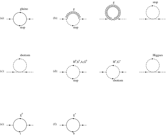
Figure 2: One-loop self-energy diagrams for the stops $(i,j=1,2)$: a) $i\Pi^{\tilde{g}}_{ij}$; b) $i\Pi^{\tilde{t}}_{ij}$; c) $i\Pi^{\tilde{b}}_{ij}$; d) $i\Pi^{H}_{ij}$; e) $i\Pi^{\tilde{\chi}^{0}}_{ij}$; f) $i\Pi^{\tilde{\chi}^{+}}_{ij}$.

The self-energies have been calculated both in the Feynman and in the Landau gauge, with the same results. As usual, in order to explicitly preserve supersymmetry, we have adopted the $\overline{DR}$ scheme [5]. The complete results for the one-loop self-energies of the top, the two stops and the gluino are reported in appendix A.

It can be seen by looking at the formulae that some new parameters must be introduced in order to calculate the full one-loop expressions. The independent parameters that must be added to the ones that appear in the tree-level relations are $\alpha_{s},m_{A}$ and $\tilde{m}_{B}$, where $m_{A}$ is the physical mass of the CP-odd neutral Higgs boson and $\tilde{m}_{B}$ is the soft mass term for the right sbottom squark. The masses of the other Higgs bosons ($H^{0},h^{0}$ and $H^{\pm}$) and the CP-even mixing angle $\alpha$ can be deduced with tree-level relations from $m_{A},m_{Z},m_{W}$ and $\tan\beta$. The masses of the sbottoms can be obtained from $\tilde{m}_{Q},\tilde{m}_{B},m_{Z},m_{W}$ and $\tan\beta$. All these tree-level relations can be found in the literature.

We have verified that the inclusion of terms proportional to $g$ and $g^{\prime}$ (namely, $m^{2}_{Z}$ and $m^{2}_{W}$) in the tree-level relations for the masses of the particles circulating in the loops does not significantly modify the results. For this reason, we have neglected them in the tree-level relations for the charginos and neutralinos mass matrices. This further approximation greatly simplifies the numerical implementation of the general formulae reported in appendix A. The charginos and neutralinos eigenvalues in this approximation are:

$$\tilde{m}_{\chi^{+}_{i}} = (M_{2},\mu)\ \qquad\qquad\qquad i=1,2,$$ (18)

$$\tilde{m}_{\chi^{0}_{j}} = (M_{1},M_{2},\mu,-\mu)\ \ \qquad j=1,4,$$ (19)

while the rotation matrices are:

$$V_{ij} = \left(\begin{array}[]{cc}1&0\\ 0&1\end{array}\right),$$ (22)

$$N_{ij} = \left(\begin{array}[]{cccc}1&0&0&0\\ 0&1&0&0\\ 0&0&\frac{1}{\sqrt{2}}&-\frac{1}{\sqrt{2}}\\ 0&0&\frac{1}{\sqrt{2}}&\frac{1}{\sqrt{2}}\end{array}\right).$$ (27)

In this approximation it can be seen, by looking at the formulae reported in appendix A, that the gaugino soft masses $M_{1},M_{2}$ do not appear explicitly. Therefore they have not been included in the input parameters set.

Figure 3: One-loop self-energy diagrams for the gluino: a) $i\Pi^{\tilde{g}}_{\tilde{g}}$; b) $i\Pi^{\tilde{t}}_{\tilde{g}}$; c) $i\Pi^{\tilde{b}}_{\tilde{g}}$.

In our approximation the electroweak gauge couplings $g$ and $g^{\prime}$ (equivalent to $\sin^{2}\theta_{W}$ and $\alpha_{em}$) do not evolve under the renormalization group equations. They have been fixed at the values $\sin^{2}\theta_{W}=0.23$ and $\alpha_{em}=\frac{1}{128}$. Another fixed input parameter is the $Z^{0}$ physical mass, $m_{Z}=91.18$ GeV. The other two couplings ($\alpha_{s},h_{t}$) have been chosen in order to give, at the electroweak scale, a value for the top pole mass that lies approximately in the experimental range. We stress that all the input parameters must be interpreted as MSSM parameters: e.g. $\alpha_{s}$ is the MSSM strong coupling constant, and not the SM one.

In order to compare our full one-loop calculations with the results obtained in the leading-log approximation via the renormalization group equations, we have used the explicit solution of the RGEs that can be found in their general form in [6]. In our approximation we must neglect terms proportional to dimensionless couplings other than $g_{s},h_{t}$ also in the RGEs, which therefore can be explicitly solved. The details of the RGEs solutions are reported in appendix B. It must be noted that in those formulae another two parameters (deducible from the already discussed set) appear, $v_{2}$ and $\tilde{m}_{H_{2}}$. For consistency, their expression in terms of the input parameters has been calculated at the one-loop level. To extract from the input parameters the one-loop VEV $v_{2}$, we have calculated the running $\overline{DR}$ mass $m^{2}_{Z}(Q)$ from the physical $Z^{0}$ mass $m_{Z}$ using the following relation:

$$m^{2}_{Z}(Q)=m^{2}_{Z}+\left.\Pi_{Z}(p^{2},Q)\right|_{p^{2}=m^{2}_{Z}}.$$ (28)

In the already obtained expression for the one-loop self-energy $\Pi_{Z}$ [7], we have kept only terms $O(g^{2})$ to implement our approximation. The Feynman graphs that contribute to the $Z^{0}$ self-energy in this approximation are reported in fig. 4. The decomposition of $\Pi_{Z}$ on the subsets of graphs is:

$$-ig^{\mu\nu}\Pi_{Z}(p^{2})=-ig^{\mu\nu}\left[\Pi^{f}_{Z}(p^{2})+\Pi^{\tilde{\chi}^{0}}_{Z}(p^{2})+\Pi^{\tilde{\chi}^{+}}_{Z}(p^{2})+\Pi^{H}_{Z}(p^{2})\right].$$ (29)

The one-loop expression is presented for completeness in appendix A, jointly with our new one-loop results. The one-loop VEV $v_{2}$ is then obtained from $m^{2}_{Z}(Q)$ and $\tan\beta$ with the tree-level relation (3). This procedure corresponds to the minimization of the one-loop effective potential: with this definition of the VEVs, the one-loop tadpole terms disappear (as the tree-level tadpoles disappear as a consequence of the tree-level scalar potential minimization). To extract from the input parameters the one-loop value for $\tilde{m}_{H_{2}}$, we have used the one-loop expressions that relate $\tilde{m}_{H_{1}},\tilde{m}_{H_{2}}$ and $m_{Z},m_{A}$ presented in eqs. (22),(23) and (24) of [8].

Figure 4: One-loop self-energy diagrams for the $Z^{0}$: a) $-ig^{\mu\nu}\Pi^{f}_{Z}$; b) $-ig^{\mu\nu}\Pi^{H}_{Z}$; c) $-ig^{\mu\nu}\Pi^{\tilde{\chi}^{0}}_{Z}$; d) $-ig^{\mu\nu}\Pi^{\tilde{\chi}^{+}}_{Z}$.

In the case of the stop squarks we have verified, as a check of the calculation, that the quadratic divergence of the sum of the full set of graphs is zero, as it should be in a softly broken supersymmetric theory. As a further check, we have verified analytically for all the studied masses that the implicit $Q$-dependence of the running mass cancels with the explicit $Q$-dependence of the one-loop self-energy. The logarithmic dependence on $Q$ for the renormalized gluino mass has also been checked by a comparison with the results in [9]. The one-loop correction to the top quark mass (including the finite part) in the $\overline{DR}$ scheme for the terms proportional to $g_{s}$ has been compared with [10]. As a consistency check, we have verified that if the off-diagonal contributions $O(\hbar^{2})$ in eq. (9) are kept the one-loop-corrected pole masses do not significantly change.

3 Numerical analysis

In this section we describe in some detail the numerical results obtained for the one-loop-corrected masses of the top, the two stops and the gluino.

In fig. 5 we report the scale-dependence of the $\overline{DR}$ running masses (dashed lines) and of the one-loop-corrected pole masses (solid lines). Our representative choice of parameters, assigned conventionally at the scale $Q_{0}=1000$ GeV, is: $\tilde{m}_{Q}=\tilde{m}_{T}=\tilde{m}_{B}=\tilde{m}_{g}=A_{t}=\mu=m_{A}=200$ GeV; $\tan\beta=2$; it can be seen that, in all four cases, the strong $Q$-dependence of the running mass $m(Q)$ is significantly reduced. This is an expected feature, due to the analytic cancellation of the logarithmic dependence in $Q$ between the running expression and the one-loop self-energy. It must be noted that the residual scale-dependence present in figs. 5b and 5c can be explained in the following way: using in the numerical calculations the neutralino and chargino masses reported in eqs. (18) and (19), we introduce a partial non-cancellation of the scale-dependence between $\tilde{m}^{2}_{t_{i}}(Q)$ and $\Pi_{ii}(\tilde{m}^{2}_{t_{i}},Q)$. Due to the improved scale-independence, one can check if the usual procedure adopted to choose the optimal scale to evaluate the running mass ($Q\simeq m$) can lead to a wrong calculation of the one-loop effects. This is actually the case, as can be seen for example for the gluino or the lightest stop mass.

Figure 5: Scale-dependence for the one-loop-corrected masses: a) $t$; b) $\tilde{t}_{1}$; c) $\tilde{t}_{2}$; d) $\tilde{g}$. The solid lines represent the complete one-loop results, while the dashed lines are the running $\overline{DR}$ masses.

Now we can start a detailed analysis of the complete results, comparing them with the running masses obtained at the “natural” scale $Q\simeq m$. We find that in many cases the largest corrections to the running masses come from the loops in which a gluino is circulating. Therefore we report, for all four masses under consideration, the dependence of the one-loop-corrected mass on the gluino mass. We present also the dependence on other parameters in various interesting cases.

1. In fig. 6 we report the one-loop-corrected mass for the top. We have verified that the top mass corrections are almost independent from $m_{A}$, which has then been kept fixed at $m_{A}=300$ GeV. The corrections have been calculated at the “natural” scale of $Q=170$ GeV. We have studied two main situations: the case in which the two stop states are almost degenerate and the case in which the lightest stop state is “very” light (between the experimental lower bounds of $\simeq 50$ GeV and 100 GeV). To obtain degenerate stop states, we have chosen universal soft mass terms ($\tilde{m}_{Q}=\tilde{m}_{T}=\tilde{m}_{B}=\tilde{m}_{U}$) for the squark and $A_{t}=\mu\cot\beta=250$ GeV. This case is illustrated in fig. 6a, for four representative values of $\tilde{m}_{U}$, ($\tilde{m}_{U}=100,200,400,600$ GeV). In the same situation, we have studied the dependence on $\tan\beta$. The results are reported in fig. 6b, with $\tilde{m}_{g}=300$ GeV, $\tan\beta=$1–50. To obtain a light stop state, we have still chosen universal soft mass terms ($\tilde{m}_{Q}=\tilde{m}_{T}=\tilde{m}_{B}=\tilde{m}_{U}$) for the squark, but $A_{t}=0$. The dependence of the top mass on $m_{A}$ in this situation is reported in fig. 6c, with $m_{A}=$200–600 GeV. In these last two figs. $\tilde{m}_{U}=200,400,600$ GeV. It can be seen that in all the cases presented, the corrections to the running top mass are quite stable and not very sensitive to the variation of the parameters. The results obtained for $\tilde{m}_{U}=150$ GeV are reported in fig. 6d. The corresponding lightest stop mass is approximately $\tilde{m}_{t_{2}}<100$ GeV. In this last figure, we have studied in detail the single contribution of the different classes of Feynman graphs to the complete result, in the case of a “very light” $\tilde{t}_{2}$. The corrections have been compared with the QCD correction (represented by the solid line that lies in the middle), which is the main SM contribution in the approximation $g=g^{\prime}=0$. The QCD correction to the running mass at $Q=170$ GeV is slightly less than 10 GeV. The dotted lines represent the different contributions added to the QCD corrections. Starting from the QCD line, we can see the charginos, neutralinos, Higgses and gluino contributions. It can be seen that the largest correction (to the QCD result) comes from the gluino loops. We stress that, in the different cases examined, the MSSM corrections can reach half (or more) of the QCD correction. Also, the complete one-loop results can significantly differ from the running ones.

   

   Figure 6: One-loop-corrected top mass (in GeV): a) as a function of the running gluino mass, for $\tilde{m}_{Q}=\tilde{m}_{T}=\tilde{m}_{B}=100,200,400,600$ GeV from the bottom; $A_{t}=250,\mu=500,m_{A}=300$ GeV; $\tan\beta=2$. b) as a function of $\tan\beta$, for $\tilde{m}_{Q}=\tilde{m}_{T}=\tilde{m}_{B}=200,400,600$ GeV from the bottom; $A_{t}=250,\mu=500,m_{A}=300$; $\tilde{m}_{g}=300$ GeV. c) as a function of $m_{A}$, for $\tilde{m}_{Q}=\tilde{m}_{T}=\tilde{m}_{B}=200,400,600$ GeV from the bottom; $A_{t}=0,\mu=500$, $\tilde{m}_{g}=300$ GeV; $\tan\beta=2$. d) as a function of the running gluino mass, for $\tilde{m}_{Q}=\tilde{m}_{T}=\tilde{m}_{B}=150$ GeV; $A_{t}=0,\mu=500,m_{A}=300$ GeV; $\tan\beta=2$. The solid lines are the complete result, the dashed ones represent the running mass. In (d), the lower solid line is the pure QCD correction; the dotted lines represent the contributions of (starting from the bottom) charginos, neutralinos, Higgses and gluino loops added to the pure QCD correction.

2. In fig. 7 we report the results for the “heaviest” stop state $\tilde{t}_{1}$. Also for this particle we have studied the two cases of almost degenerate stop states and of a “very light” $\tilde{t}_{2}$. In fig. 7a we consider the case of degenerate stop states at three different values of the universal soft mass term $\tilde{m}_{U}=100,200,400$ GeV. As usual the dashed lines represent the running masses. The three results have been obtained at the “natural” scales $Q=150,240,430$ GeV. In figs. 7b and 7d we have reported on the dependence on $m_{A}$ and $\mu$ in the case of a “very light” $\tilde{t}_{2}$ at the scale $Q=300$ GeV (with $\tilde{m}_{U}=170$ GeV, $A_{t}=0,\tilde{m}_{g}=300$ GeV). In particular, in 7b $\mu=500$ GeV and $m_{A}=$200–600 GeV while in 7d $m_{A}=500$ GeV and $\mu=$200–600 GeV. In fig. 7c, is reported on the dependence of $\tilde{m}_{t_{1}}$ on the gluino mass in the same situation, with $\tilde{m}_{U}=200$ GeV and $Q=320$ GeV. In this case, we have studied also the contributions coming from the different loops. The horizontal dotted lines are (from the bottom) the neutralinos, charginos, Higgses, sbottoms and stops contributions, while the dotted line that follows the complete result is the gluino contribution. It can be easily seen that also in this case the most important contribution comes from the gluino loops. Actually, in all the cases that we have observed, the corrections to the $\tilde{m}_{t_{1}}$ running mass are not very large. We have seen that for almost degenerate running states, the one-loop-corrected masses can be interchanged (namely, $\tilde{t}_{2}$ can become the heaviest stop state).

   

   Figure 7: One-loop-corrected $\tilde{t}_{1}$ mass (in GeV): a) as a function of the running gluino mass, for $\tilde{m}_{Q}=\tilde{m}_{T}=\tilde{m}_{B}=100,200,400$ GeV from the bottom; $A_{t}=250,\mu=500,m_{A}=300$ GeV; $\tan\beta=2$. b) as a function of $m_{A}$, for $\tilde{m}_{Q}=\tilde{m}_{T}=\tilde{m}_{B}=170$ GeV; $A_{t}=0,\mu=500$, $\tilde{m}_{g}=300$ GeV; $\tan\beta=2$. c) as a function of the running gluino mass, for $\tilde{m}_{Q}=\tilde{m}_{T}=\tilde{m}_{B}=200$ GeV; $A_{t}=0,\mu=500,m_{A}=500$ GeV; $\tan\beta=2$. d) as a function of $\mu$, for $\tilde{m}_{Q}=\tilde{m}_{T}=\tilde{m}_{B}=170$ GeV; $A_{t}=0,m_{A}=500$, $\tilde{m}_{g}=300$ GeV; $\tan\beta=2$. The solid lines are the complete result, the dashed ones represent the running mass. In fig. (c) the horizontal dotted lines represent the contributions of (starting from the bottom) Higgses, sbottoms, charginos, neutralinos and stops loops. The dotted line with the same shape as the complete result is the gluino contribution.

3. In fig. 8 we report the results for $\tilde{m}_{t_{2}}$ with the same choices of parameters as for $\tilde{m}_{t_{1}}$. In fig. 8a, it can be seen that $\tilde{t}_{2}$ has a behaviour quite similar to $\tilde{t}_{1}$: actually, the one-loop corrections can interchange the two states ($\tilde{t}_{2}$ can become the heaviest one). Also for $\tilde{t}_{2}$, the corrections to the running mass (evaluated at the same “natural” scales) are quite small. In figs. 8b, 8c and 8d we have studied the case of a “very light” $\tilde{t}_{2}$, at the “natural” scale $Q=100$ GeV. It can be seen in all three figures that the one-loop corrections significantly modify the renormalization-group-improved tree-level results. The most interesting situation is reported in fig. 8c. At the “natural” scale of $Q=100$ GeV, we have chosen a universal soft mass term $\tilde{m}_{U}=200$ GeV, in order to get a sufficiently heavy running mass, $\tilde{m}_{t_{2}}(Q)\simeq 150$ GeV. It can be seen from the figure that the one-loop-corrected mass is significantly different from the running mass, and that can easily fall below the experimental lower bound of $\simeq 50$ GeV also for a non-super-heavy gluino mass. This implies that in the case of a light stop state the running-mass result must be used (also at the “natural” scale) with great care. As usual, we have studied the different contributions to this case. Starting from the bottom, the horizontal dotted lines are the contributions coming from neutralinos, charginos, sbottoms, stops and Higgses loops. The dotted line with the same shape as the complete result represents the gluino contribution.

   

   Figure 8: One-loop-corrected $\tilde{t}_{2}$ mass (in GeV): a) as a function of the running gluino mass, for $\tilde{m}_{Q}=\tilde{m}_{T}=\tilde{m}_{B}=100,200,400$ GeV from the bottom; $A_{t}=250,\mu=500,m_{A}=300$ GeV; $\tan\beta=2$. b) as a function of $m_{A}$, for $\tilde{m}_{Q}=\tilde{m}_{T}=\tilde{m}_{B}=170$ GeV; $A_{t}=0,\mu=500$, $\tilde{m}_{g}=300$ GeV; $\tan\beta=2$. c) as a function of the running gluino mass, for $\tilde{m}_{Q}=\tilde{m}_{T}=\tilde{m}_{B}=200$ GeV; $A_{t}=0,\mu=500,m_{A}=500$ GeV; $\tan\beta=2$. d) as a function of $\mu$, for $\tilde{m}_{Q}=\tilde{m}_{T}=\tilde{m}_{B}=170$ GeV; $A_{t}=0,m_{A}=500$, $\tilde{m}_{g}=300$ GeV; $\tan\beta=2$. The solid lines are the complete result, the dashed ones represent the running mass. In fig. (c), the horizontal dotted lines represent the contributions of (starting from the bottom) neutralinos, charginos, sbottoms, stops and Higgses loops. The dotted line with the same shape as the complete result is the gluino contribution.

4. In fig. 9 we report the results for the one-loop-corrected gluino mass in two different cases: a heavy gluino and a massless gluino. Our results agree with the one-loop corrections calculated in [11], and contain as a particular case the results of [12] for a gluino massless at tree level. In 9a and 9b we have studied the dependence on $\mu$ and $\tan\beta$ of the corrections to a heavy gluino mass, for a running mass $\tilde{m}_{g}=300$ GeV at the “natural” scale $Q=300$ GeV. It has been found that the corrections increase with increasing scalar soft mass terms $\tilde{m}_{Q},\tilde{m}_{T},\tilde{m}_{B}$, and with decreasing $\tan\beta$. They can be of order 10–30% of the running mass, for stop masses not exceeding 1 TeV. In figs. 9c and 9d we report results for the massless case (for which we have used $\alpha_{s}=0.15$). Here the situation is reversed, and the corrections increase with decreasing scalar soft mass terms. It is well known that for a massless gluino the corrections at one loop are proportional to the mass differences between the squarks. This has been verified by giving non-universal soft mass terms, keeping the average scale $\tilde{m}_{U}$ at a small value. We have seen that, at the “natural” scale $Q=1$ GeV, the corrections to a zero mass gluino can reach 3 or 4 GeV. Comparing our results with those presented in [12], we note that we have explored a different region of the parameters space.

   

   
   

   Figure 9: One-loop-corrected gluino mass (in GeV): a) as a function of $\mu$, for $\tilde{m}_{Q}=\tilde{m}_{T}=\tilde{m}_{B}=200,300,400$ GeV from the bottom; $A_{t}=0,m_{A}=500$ GeV; $\tan\beta=2$. b) as a function of $\tan\beta$, for $\tilde{m}_{Q}=\tilde{m}_{T}=\tilde{m}_{B}=200,300,400$ GeV from the bottom; $A_{t}=0,m_{A}=500,\mu=500$ GeV. c) as a function of $\mu$, for $\tilde{m}_{Q}=\tilde{m}_{T}=\tilde{m}_{B}=300,200,150,100,50$ GeV from the bottom; $A_{t}=0,m_{A}=500$ GeV; $\tan\beta=2$. d) as a function of $\tan\beta$, for $\tilde{m}_{Q}=\tilde{m}_{T}=\tilde{m}_{B}=300,200,150,100$ GeV from the bottom; $A_{t}=0,m_{A}=500,\mu=500$ GeV. The solid lines are the complete result, the dashed ones represent the running mass.

Appendix A: One-loop results

In this appendix we report all the explicit results for the one-loop radiative corrections to the pole masses of the stops, of the gluino and of the top quark, obtained in the approximation where all the dimensionless couplings other than $g_{s}$ and $h_{t}$ are set to zero. The corresponding Feynman rules have been deduced from the rules reported in [2, 4]. It must be noticed that (in the last of [2]) a factor $\frac{1}{2}$ is missing in the vertices between two neutral Higgses and two squarks. This factor, due to a combinatorial factor of 2, cancels if the external legs are the two neutral Higgses giving the Feynman rule reported in the same reference. The same happens to the two-gluon/two-squark vertex. In the formulae we have made use of the following integrals:

$$F(1,2,3) = {\cal R}e\int^{1}_{0}dz\log\left(\frac{T(1,2,3)}{Q^{2}}\right)$$

$$H(1,2,3) = {\cal R}e\int^{1}_{0}dz[m^{2}_{1}(1-z)+m^{2}_{2}z]\log\left(\frac{T(1,2,3)}{Q^{2}}\right)$$

$$G(1,2,3) = {\cal R}e\int^{1}_{0}dz[m^{2}_{3}z(1-z)]\log\left(\frac{T(1,2,3)}{Q^{2}}\right)$$

$$K(1,2,3) = {\cal R}e\int^{1}_{0}dz[m^{2}_{3}z(1-z)-m^{2}_{1}(1-z)-m^{2}_{2}z]\log\left(\frac{T(1,2,3)}{Q^{2}}\right)$$

$$L(1,2,3) = {\cal R}e\int^{1}_{0}dz[m^{2}_{3}(z-2)^{2}]\log\left(\frac{T(1,2,3)}{Q^{2}}\right)$$

$$M(1,2,3) = {\cal R}e\int^{1}_{0}dz[m_{3}z]\log\left(\frac{T(1,2,3)}{Q^{2}}\right)$$

$$N(1,2,3) = {\cal R}e\int^{1}_{0}dz[m_{3}(1-z)]\log\left(\frac{T(1,2,3)}{Q^{2}}\right)$$

where $T(1,2,3)=m^{2}_{1}(1-z)+m^{2}_{2}z-m^{2}_{3}z(1-z)-i\epsilon^{\prime}$. The analytical expressions for these integrals can be found following [13]. They all depend on:

$$F(1,2,3)=-2+\log\left(\frac{m_{1}m_{2}}{Q^{2}}\right)+\frac{m^{2}_{1}-m^{2}_{2}}{m^{2}_{3}}log\left(\frac{m_{1}}{m_{2}}\right)$$

$$+\frac{1}{m^{2}_{3}}\sqrt{\mid(m_{1}+m_{2})^{2}-m^{2}_{3}\mid\mid(m_{1}+m_{2})^{2}-m^{2}_{3}\mid}f(1,2,3)$$

where

$$f(1,2,3)=\left\{\begin{array}[]{ll}\log\frac{\sqrt{(m_{1}+m_{2})^{2}-m^{2}_{3}}-\sqrt{(m_{1}-m_{2})^{2}-m^{2}_{3}}}{\sqrt{(m_{1}+m_{2})^{2}-m^{2}_{3}}+\sqrt{(m_{1}-m_{2})^{2}-m^{2}_{3}}}&{\rm if}\ \ m^{2}_{3}\leq(m_{1}-m_{2})^{2}\\ \\ 2\arctan\frac{m^{2}_{3}-(m_{1}-m_{2})^{2}}{(m_{1}+m_{2})^{2}-m^{2}_{3}}&{\rm if}\ \ (m_{1}-m_{2})^{2}<m^{2}_{3}<(m_{1}+m_{2})^{2}\\ \\ \log\frac{\sqrt{m^{2}_{3}-(m_{1}-m_{2})^{2}}+\sqrt{m^{2}_{3}-(m_{1}+m_{2})^{2}}}{\sqrt{m^{2}_{3}-(m_{1}-m_{2})^{2}}-\sqrt{m^{2}_{3}-(m_{1}+m_{2})^{2}}}&{\rm if}\ \ m^{2}_{3}\geq(m_{1}+m_{2})^{2}\end{array}\right.$$ (30)

The other integrals have the following analytical expressions:

$$H(1,2,3) = \frac{m^{2}_{1}-m^{2}_{2}}{m^{2}_{3}}\left[m^{2}_{1}\left(\log\frac{m^{2}_{1}}{Q^{2}}-1\right)-m^{2}_{2}\left(\log\frac{m^{2}_{2}}{Q^{2}}-1\right)\right]$$

$$+ \frac{1}{2}\left[m^{2}_{1}+m^{2}_{2}-\left(\frac{m^{2}_{1}-m^{2}_{2}}{m_{3}}\right)^{2}\right]F(1,2,3)$$

$$G(1,2,3) = \frac{m^{2}_{3}}{18}-\frac{1}{6}\left[m^{2}_{1}\log\frac{m^{2}_{1}}{Q^{2}}+m^{2}_{2}\log\frac{m^{2}_{2}}{Q^{2}}\right]+\frac{2}{3}H(1,2,3)$$

$$- \frac{1}{6}[m^{2}_{1}+m^{2}_{2}-m^{2}_{3}]F(1,2,3)$$

$$K(1,2,3) = G(1,2,3)-H(1,2,3)$$

$$L(1,2,3) = m^{2}_{3}\left(4-\frac{3m^{2}_{1}}{m^{2}_{1}-m^{2}_{2}}\right)F(1,2,3)+\frac{3m^{2}_{3}}{m^{2}_{1}-m^{2}_{2}}H(1,2,3)-G(1,2,3)$$

$$M(1,2,3) = \frac{m_{3}m^{2}_{1}}{m^{2}_{1}-m^{2}_{2}}F(1,2,3)-\frac{m_{3}}{m^{2}_{1}-m^{2}_{2}}H(1,2,3)$$

$$N(1,2,3) = m_{3}F(1,2,3)-M(1,2,3)$$

All these integrals are symmetric under the permutation $1\rightarrow 2$, made exception for $L$ and for $M(1,2,3)=N(2,1,3)$. It has been stressed [13] that if some entries of the integral $F$ are zero, the right expressions are not deducible by just taking the limit from these formulae. This happens because, if $T(1,2,3)$ has some zero entries, some of the poles in the logarithm may disappear. Here we report the main particular cases, for completeness:

$$F(1,2,0) = -1+\frac{1}{m^{2}_{1}-m^{2}_{2}}\left[m^{2}_{1}\log\frac{m^{2}_{1}}{Q^{2}}-m^{2}_{2}\log\frac{m^{2}_{2}}{Q^{2}}\right]$$

$$F(1,1,0) = \log\frac{m^{2}_{1}}{Q^{2}}.$$

The particular cases for the other integrals are deducible by taking the limit for the reported expressions and using the particular expressions for the $F$ integral. This is not true for the $L,M,N$ integrals in the case $m_{1}=m_{2}$: but also in the pathological case their decomposition over the main integrals $F,H,G$ is easy to obtain. Below are reported the expressions for the one-loop radiative corrections to the pole masses of the stops, the gluino and the top quark. In these expressions, $N$ is the number of colours ($N=3$), $(\alpha,\beta)=1,2,3$ and $(a,b)=1,\dots,8$. Moreover, $C_{2}(R)=\frac{N^{2}-1}{2N}$ and $C_{2}(G)=N$. We have used a subscript $c$ for the up-type quarks and squarks different from top and stop, and a subscript $b$ for all the down-type quarks and squarks. In the following, ($\sin\phi_{q},\cos\phi_{q}$) will be abbreviated as ($s_{q},c_{q}$).

1. Self-energy of the top quark (see fig. 1):

   $$i\Pi^{t}_{t}(\mbox{$\not\!\!p$}) =-\frac{i\delta^{\alpha\beta}}{16\pi^{2}}g^{2}_{s}C_{2}(R) \left[2N(0,t,p)-4m_{t}F(0,t,p)\right]$$

   $$i\Pi^{\tilde{g}}_{t}(\mbox{$\not\!\!p$}) =-\frac{i\delta^{\alpha\beta}}{16\pi^{2}}g^{2}_{s}C_{2}(R) \left[M(\tilde{g},\tilde{t}_{1},p)-2\tilde{m}_{g}s_{t}c_{t}F(\tilde{g},\tilde{t}_{1},p)\right.$$

   $$+\left.M(\tilde{g},\tilde{t}_{2},p)+2\tilde{m}_{g}s_{t}c_{t}F(\tilde{g},\tilde{t}_{2},p)\right]$$

   $$i\Pi^{H}_{t}(\mbox{$\not\!\!p$}) =-\frac{i\delta^{\alpha\beta}}{16\pi^{2}}h^{2}_{t} \left\{\frac{1}{2}\sin^{2}\alpha\left[N(H^{0},t,p)+m_{t}F(H^{0},t,p))\right]\right.$$

   $$+\frac{1}{2}\cos^{2}\alpha\left[N(h^{0},t,p)+m_{t}F(h^{0},t,p)\right]$$

   $$+\frac{1}{2}\cos^{2}\beta\left[N(A,t,p)-m_{t}F(A,t,p)\right]$$

   $$+\frac{1}{2}\sin^{2}\beta\left[N(0,t,p)-m_{t}F(0,t,p)\right]$$

   $$+\left.\frac{1}{2}\left[\cos^{2}\beta M(H^{\pm},b,p)+\sin^{2}\beta M(0,b,p)\right]\right\}$$

   $$i\Pi^{\tilde{\chi}^{0}}_{t}(\mbox{$\not\!\!p$}) =-\frac{i\delta^{\alpha\beta}}{16\pi^{2}}h^{2}_{t} \left\{\frac{1}{2}\sum_{j}\left[\mid N_{j4}\mid^{2}M(\tilde{\chi}^{0}_{j},\tilde{t}_{1},p)+\tilde{m}_{\chi^{0}_{j}}s_{t}c_{t}(N^{2}_{j4}+N^{\star^{2}}_{j4})F(\tilde{\chi}^{0}_{j},\tilde{t}_{1},p)\right]\right.$$

   $$+\left.\frac{1}{2}\sum_{j}\left[\mid N_{j4}\mid^{2}M(\tilde{\chi}^{0}_{j},\tilde{t}_{2},p)-\tilde{m}_{\chi^{0}_{j}}s_{t}c_{t}(N^{2}_{j4}+N^{\star^{2}}_{j4})F(\tilde{\chi}^{0}_{j},\tilde{t}_{2},p)\right]\right\}$$

   $$i\Pi^{\tilde{\chi}^{+}}_{t}(\mbox{$\not\!\!p$}) =-\frac{i\delta^{\alpha\beta}}{16\pi^{2}}h^{2}_{t} \left\{\frac{1}{2}\sum_{i}\left[c^{2}_{b}\mid V_{i2}\mid^{2}M(\tilde{\chi}^{+}_{i},\tilde{b}_{1},p)+s^{2}_{b}\mid V_{i2}\mid^{2}M(\tilde{\chi}^{+}_{i},\tilde{b}_{2},p)\right]\right\}$$

2. Self-energies of the stops (see fig. 2):

   1. $$i\Pi^{\tilde{g}}_{11} =\frac{i\delta^{\alpha\beta}}{16\pi^{2}} g^{2}_{s}C_{2}(R)\left[\frac{2}{3}p^{2}-2(m^{2}_{t}+m^{2}_{\tilde{g}})\right.$$

      $$-\left.8K(\tilde{g},t,p)-4G(\tilde{g},t,p)-8s_{t}c_{t}m_{t}\tilde{m}_{g}F(\tilde{g},t,p)\right]$$

      $$i\Pi^{\tilde{t}}_{11} =\frac{i\delta^{\alpha\beta}}{16\pi^{2}} \left\{g^{2}_{s}C_{2}(R)\left[\frac{1}{6}p^{2}+\frac{1}{2}\tilde{m}^{2}_{t_{1}}-4s^{2}_{t}c^{2}_{t}(\tilde{m}^{2}_{t_{1}}-\tilde{m}^{2}_{t_{2}})-2K(0,\tilde{t}_{1},p)\right.\right.$$

      $$+\left.L(0,\tilde{t}_{1},p)+(1-4s^{2}_{t}c^{2}_{t})K(\tilde{t}_{1},\tilde{t}_{1},0)+4s^{2}_{t}c^{2}_{t}K(\tilde{t}_{2},\tilde{t}_{2},0)\right]$$

      $$+h^{2}_{t}\left[2(N+1)s^{2}_{t}c^{2}_{t}(\tilde{m}^{2}_{t_{1}}-\tilde{m}^{2}_{t_{2}})+\tilde{m}^{2}_{t_{2}}\right.$$

      $$+\left.\left.2(N+1)s^{2}_{t}c^{2}_{t}K(\tilde{t}_{1},\tilde{t}_{1},0)+(c^{4}_{t}+s^{4}_{t}-2Ns^{2}_{t}c^{2}_{t})K(\tilde{t}_{2},\tilde{t}_{2},0)\right]\right\}$$

      $$i\Pi^{\tilde{b}}_{11} =\frac{i\delta^{\alpha\beta}}{16\pi^{2}} h^{2}_{t}\left\{s^{2}_{t}(c^{2}_{b}\tilde{m}^{2}_{b_{1}}+s^{2}_{b}\tilde{m}^{2}_{b_{2}})+s^{2}_{t}\left[c^{2}_{b}K(\tilde{b}_{1},\tilde{b}_{1},0)+s^{2}_{b}K(\tilde{b}_{2},\tilde{b}_{2},0)\right]\right\}$$

      $$i\Pi^{H}_{11} =\frac{i\delta^{\alpha\beta}}{16\pi^{2}} h^{2}_{t}\left[\frac{1}{2}m^{2}_{H^{0}}\sin^{2}\alpha+\frac{1}{2}m^{2}_{h^{0}}\cos^{2}\alpha+\frac{1}{2}m^{2}_{A}\cos^{2}\beta+s^{2}_{t}m^{2}_{H^{\pm}}\cos^{2}\beta\right.$$

      $$+\frac{1}{2}\sin^{2}\alpha K(H^{0},H^{0},0)+\frac{1}{2}\cos^{2}\alpha K(h^{0},h^{0},0)$$

      $$+\frac{1}{2}\cos^{2}\beta K(A,A,0)+s^{2}_{t}\cos^{2}\beta K(H^{\pm},H^{\pm},0)$$

      $$-2m^{2}_{t}(V^{H^{0}}_{11})^{2}F(H^{0},\tilde{t}_{1},p)-2m^{2}_{t}(V^{H^{0}}_{12})^{2}F(H^{0},\tilde{t}_{2},p)$$

      $$-2m^{2}_{t}(V^{h^{0}}_{11})^{2}F(h^{0},\tilde{t}_{1},p)-2m^{2}_{t}(V^{h^{0}}_{12})^{2}F(h^{0},\tilde{t}_{2},p)$$

      $$-\frac{1}{2}\sin^{2}\beta(V^{A}_{12})^{2}F(A,\tilde{t}_{2},p)-\frac{1}{2}\sin^{2}\beta(V^{G^{0}}_{12})^{2}F(0,\tilde{t}_{2},p)$$

      $$-\sin^{2}\beta(V^{H^{\pm}}_{11})^{2}F(H^{\pm},\tilde{b}_{1},p)-\sin^{2}\beta(V^{H^{\pm}}_{12})^{2}F(H^{\pm},\tilde{b}_{2},p)$$

      $$-\left.\sin^{2}\beta(V^{G^{\pm}}_{11})^{2}F(0,\tilde{b}_{1},p)-\sin^{2}\beta(V^{G^{\pm}}_{12})^{2}F(0,\tilde{b}_{2},p)\right]$$

      $$i\Pi^{\tilde{\chi}^{0}}_{11} =\frac{i\delta^{\alpha\beta}}{16\pi^{2}} h^{2}_{t}\left[\frac{1}{3}p^{2}-m^{2}_{t}-\sum_{j}\mid N_{j4}\mid^{2}\tilde{m}^{2}_{\chi^{0}_{j}}\right.$$

      $$-4\sum_{j}\mid N_{j4}\mid^{2}K(\tilde{\chi}^{0}_{j},t,p)-2\sum_{j}\mid N_{j4}\mid^{2}G(\tilde{\chi}^{0}_{j},t,p)$$

      $$+\left.2s_{t}c_{t}\sum_{j}(N^{2}_{j4}+N^{\star^{2}}_{j4})m_{t}\tilde{m}_{\chi^{0}_{j}}F(\tilde{\chi}^{0}_{j},t,p)\right]$$

      $$i\Pi^{\tilde{\chi}^{+}}_{11} =\frac{i\delta^{\alpha\beta}}{16\pi^{2}} h^{2}_{t}\left[\frac{1}{3}s^{2}_{t}p^{2}-s^{2}_{t}m^{2}_{b}-s^{2}_{t}\sum_{i}\mid V_{i2}\mid^{2}\tilde{m}^{2}_{\chi^{+}_{i}}\right.$$

      $$-\left.4s^{2}_{t}\sum_{i}\mid V_{i2}\mid^{2}K(\tilde{\chi}^{+}_{i},b,p)-2s^{2}_{t}\sum_{i}\mid V_{i2}\mid^{2}G(\tilde{\chi}^{+}_{i},b,p)\right]$$

   2. $$i\Pi^{\tilde{g}}_{22} =\frac{i\delta^{\alpha\beta}}{16\pi^{2}} g^{2}_{s}C_{2}(R)\left[\frac{2}{3}p^{2}-2(m^{2}_{t}+m^{2}_{\tilde{g}})\right.$$

      $$-\left.8K(\tilde{g},t,p)-4G(\tilde{g},t,p)+8s_{t}c_{t}m_{t}\tilde{m}_{g}F(\tilde{g},t,p)\right]$$

      $$i\Pi^{\tilde{t}}_{22} =\frac{i\delta^{\alpha\beta}}{16\pi^{2}} \left\{g^{2}_{s}C_{2}(R)\left[\frac{1}{6}p^{2}+\frac{1}{2}\tilde{m}^{2}_{t_{2}}+4s^{2}_{t}c^{2}_{t}(\tilde{m}^{2}_{t_{1}}-\tilde{m}^{2}_{t_{2}})-2K(0,\tilde{t}_{2},p)\right.\right.$$

      $$+\left.L(0,\tilde{t}_{2},p)+(1-4s^{2}_{t}c^{2}_{t})K(\tilde{t}_{2},\tilde{t}_{2},0)+4s^{2}_{t}c^{2}_{t}K(\tilde{t}_{1},\tilde{t}_{1},0)\right]$$

      $$+h^{2}_{t}\left[-2(N+1)s^{2}_{t}c^{2}_{t}(\tilde{m}^{2}_{t_{1}}-\tilde{m}^{2}_{t_{2}})+\tilde{m}^{2}_{t_{1}}\right.$$

      $$+\left.\left.2(N+1)s^{2}_{t}c^{2}_{t}K(\tilde{t}_{2},\tilde{t}_{2},0)+(c^{4}_{t}+s^{4}_{t}-2Ns^{2}_{t}c^{2}_{t})K(\tilde{t}_{1},\tilde{t}_{1},0)\right]\right\}$$

      $$i\Pi^{\tilde{b}}_{22} =\frac{i\delta^{\alpha\beta}}{16\pi^{2}} h^{2}_{t}\left\{c^{2}_{t}(c^{2}_{b}\tilde{m}^{2}_{b_{1}}+s^{2}_{b}\tilde{m}^{2}_{b_{2}})+c^{2}_{t}\left[c^{2}_{b}K(\tilde{b}_{1},\tilde{b}_{1},0)+s^{2}_{b}K(\tilde{b}_{2},\tilde{b}_{2},0)\right]\right\}$$

      $$i\Pi^{H}_{22} =\frac{i\delta^{\alpha\beta}}{16\pi^{2}} h^{2}_{t}\left[\frac{1}{2}m^{2}_{H^{0}}\sin^{2}\alpha+\frac{1}{2}m^{2}_{h^{0}}\cos^{2}\alpha+\frac{1}{2}m^{2}_{A}\cos^{2}\beta+c^{2}_{t}m^{2}_{H^{\pm}}\cos^{2}\beta\right.$$

      $$+\frac{1}{2}\sin^{2}\alpha K(H^{0},H^{0},0)+\frac{1}{2}\cos^{2}\alpha K(h^{0},h^{0},0)$$

      $$+\frac{1}{2}\cos^{2}\beta K(A,A,0)+c^{2}_{t}\cos^{2}\beta K(H^{\pm},H^{\pm},0)$$

      $$-2m^{2}_{t}(V^{H^{0}}_{21})^{2}F(H^{0},\tilde{t}_{1},p)-2m^{2}_{t}(V^{H^{0}}_{22})^{2}F(H^{0},\tilde{t}_{2},p)$$

      $$-2m^{2}_{t}(V^{h^{0}}_{21})^{2}F(h^{0},\tilde{t}_{1},p)-2m^{2}_{t}(V^{h^{0}}_{22})^{2}F(h^{0},\tilde{t}_{2},p)$$

      $$-\frac{1}{2}\sin^{2}\beta(V^{A}_{12})^{2}F(A,\tilde{t}_{1},p)-\frac{1}{2}\sin^{2}\beta(V^{G^{0}}_{12})^{2}F(0,\tilde{t}_{1},p)$$

      $$-\sin^{2}\beta(V^{H^{\pm}}_{21})^{2}F(H^{\pm},\tilde{b}_{1},p)-\sin^{2}\beta(V^{H^{\pm}}_{22})^{2}F(H^{\pm},\tilde{b}_{2},p)$$

      $$-\left.\sin^{2}\beta(V^{G^{\pm}}_{21})^{2}F(0,\tilde{b}_{1},p)-\sin^{2}\beta(V^{G^{\pm}}_{22})^{2}F(0,\tilde{b}_{2},p)\right]$$

      $$i\Pi^{\tilde{\chi}^{0}}_{22} =\frac{i\delta^{\alpha\beta}}{16\pi^{2}} h^{2}_{t}\left[\frac{1}{3}p^{2}-m^{2}_{t}-\sum_{j}\mid N_{j4}\mid^{2}\tilde{m}^{2}_{\chi^{0}_{j}}\right.$$

      $$-4\sum_{j}\mid N_{j4}\mid^{2}K(\tilde{\chi}^{0}_{j},t,p)-2\sum_{j}\mid N_{j4}\mid^{2}G(\tilde{\chi}^{0}_{j},t,p)$$

      $$-\left.2s_{t}c_{t}\sum_{j}(N^{2}_{j4}+N^{\star^{2}}_{j4})m_{t}\tilde{m}_{\chi^{0}_{j}}F(\tilde{\chi}^{0}_{j},t,p)\right]$$

      $$i\Pi^{\tilde{\chi}^{+}}_{22} =\frac{i\delta^{\alpha\beta}}{16\pi^{2}} h^{2}_{t}\left[\frac{1}{3}c^{2}_{t}p^{2}-c^{2}_{t}m^{2}_{b}-c^{2}_{t}\sum_{i}\mid V_{i2}\mid^{2}\tilde{m}^{2}_{\chi^{+}_{i}}\right.$$

      $$-\left.4c^{2}_{t}\sum_{i}\mid V_{i2}\mid^{2}K(\tilde{\chi}^{+}_{i},b,p)-2c^{2}_{t}\sum_{i}\mid V_{i2}\mid^{2}G(\tilde{\chi}^{+}_{i},b,p)\right]$$

   3. $$i\Pi^{\tilde{g}}_{12} =\frac{i\delta^{\alpha\beta}}{16\pi^{2}} g^{2}_{s}C_{2}(R)\cos 2\phi_{t}\left[-4m_{t}\tilde{m}_{g}F(\tilde{m}_{g},t,p)\right]$$

      $$i\Pi^{\tilde{t}}_{12} =\frac{i\delta^{\alpha\beta}}{16\pi^{2}} \left\{g^{2}_{s}C_{2}(R)\cos 2\phi_{t}\left[-s_{t}c_{t}(\tilde{m}^{2}_{t_{1}}-\tilde{m}^{2}_{t_{2}})\right.\right.$$

      $$-\left.2s_{t}c_{t}(K(\tilde{t}_{1},\tilde{t}_{1},0)-K(\tilde{t}_{2},\tilde{t}_{2},0))\right]$$

      $$+h^{2}_{t}\left[(N+1)s_{t}c_{t}\cos 2\phi_{t}(\tilde{m}^{2}_{t_{1}}-\tilde{m}^{2}_{t_{2}})\right.$$

      $$+\left.\left.(N+1)s_{t}c_{t}\cos 2\phi_{t}(K(\tilde{t}_{1},\tilde{t}_{1},0)-K(\tilde{t}_{2},\tilde{t}_{2},0))\right]\right\}$$

      $$i\Pi^{\tilde{b}}_{12} =\frac{i\delta^{\alpha\beta}}{16\pi^{2}} h^{2}_{t}\left\{s_{t}c_{t}(c^{2}_{b}\tilde{m}^{2}_{b_{1}}+s^{2}_{b}\tilde{m}^{2}_{b_{2}})\right.$$

      $$+\left.s_{t}c_{t}\left[c^{2}_{b}K(\tilde{b}_{1},\tilde{b}_{1},0)+s^{2}_{b}K(\tilde{b}_{2},\tilde{b}_{2},0)\right]\right\}$$

      $$i\Pi^{H}_{12} =\frac{i\delta^{\alpha\beta}}{16\pi^{2}} h^{2}_{t}\left[m^{2}_{H^{\pm}}\cos^{2}\beta s_{t}c_{t}+\cos^{2}\beta s_{t}c_{t}K(H^{\pm},H^{\pm},0)\right.$$

      $$-2m^{2}_{t}(V^{H^{0}}_{11}V^{H^{0}}_{12})F(H^{0},\tilde{t}_{1},p)-2m^{2}_{t}(V^{H^{0}}_{12}V^{H^{0}}_{22})F(H^{0},\tilde{t}_{2},p)$$

      $$-2m^{2}_{t}(V^{h^{0}}_{11}V^{h^{0}}_{12})F(h^{0},\tilde{t}_{1},p)-2m^{2}_{t}(V^{h^{0}}_{12}V^{h^{0}}_{22})F(h^{0},\tilde{t}_{2},p)$$

      $$-\sin^{2}\beta(V^{H^{\pm}}_{11}V^{H^{\pm}}_{12})F(H^{\pm},\tilde{b}_{1},p)-\sin^{2}\beta(V^{H^{\pm}}_{12}V^{H^{\pm}}_{22})F(H^{\pm},\tilde{b}_{2},p)$$

      $$-\left.\sin^{2}\beta(V^{G^{\pm}}_{11}V^{G^{\pm}}_{12})F(0,\tilde{b}_{1},p)-\sin^{2}\beta(V^{G^{\pm}}_{12}V^{G^{\pm}}_{22})F(0,\tilde{b}_{2},p)\right]$$

      $$i\Pi^{\tilde{\chi}^{0}}_{12} =\frac{i\delta^{\alpha\beta}}{16\pi^{2}} h^{2}_{t}\left[2\sum_{j}(c^{2}_{t}N^{\star^{2}}_{j4}-s^{2}_{t}N^{2}_{j4})m_{t}\tilde{m}_{\chi^{0}_{j}}F(\tilde{\chi}^{0}_{j},t,p)\right]$$

      $$i\Pi^{\tilde{\chi}^{+}}_{12} =\frac{i\delta^{\alpha\beta}}{16\pi^{2}} h^{2}_{t}\left[\frac{2}{3}s_{t}c_{t}p^{2}-2s_{t}c_{t}m^{2}_{b}-2s_{t}c_{t}\sum_{i}\mid V_{i2}\mid^{2}\tilde{m}^{2}_{\chi^{+}_{i}}\right.$$

      $$-\left.2s_{t}c_{t}\sum_{i}\mid V_{i2}\mid^{2}(K(\tilde{\chi}^{+}_{i},b,p)+G(\tilde{\chi}^{+}_{i},b,p))\right]$$

   In these expressions, we have used the following definitions for the Higgs–squark–squark vertices in the ($\tilde{t}_{1},\tilde{t}_{2}$) basis:

   $$V^{H^{0}}_{11} = \sin\alpha+\frac{1}{m_{t}}s_{t}c_{t}(A_{t}\sin\alpha-\mu\cos\alpha)$$

   $$V^{H^{0}}_{12} = V^{H^{0}}_{21}=\frac{1}{2m_{t}}\cos 2\phi_{t}(A_{t}\sin\alpha-\mu\cos\alpha)$$

   $$V^{H^{0}}_{22} = \sin\alpha-\frac{1}{m_{t}}s_{t}c_{t}(A_{t}\sin\alpha-\mu\cos\alpha)$$

   $$V^{A}_{12} = V^{A}_{21}=(A_{t}\cot\beta+\mu)$$

   $$V^{G^{0}}_{12} = V^{G^{0}}_{21}=(A_{t}-\mu\cot\beta)$$

   $$V^{H^{\pm}}_{11} = m_{t}c_{t}c_{b}\cot\beta+s_{t}c_{b}(A_{t}\cot\beta+\mu)$$

   $$V^{H^{\pm}}_{12} = -m_{t}c_{t}s_{b}\cot\beta-s_{t}s_{b}(A_{t}\cot\beta+\mu)$$

   $$V^{H^{\pm}}_{21} = -m_{t}s_{t}c_{b}\cot\beta+c_{t}c_{b}(A_{t}\cot\beta+\mu)$$

   $$V^{H^{\pm}}_{22} = m_{t}s_{t}s_{b}\cot\beta-c_{t}s_{b}(A_{t}\cot\beta+\mu)$$

   $$V^{G^{\pm}}_{11} = m_{t}c_{t}c_{b}+s_{t}c_{b}(A_{t}-\mu\cot\beta)$$

   $$V^{G^{\pm}}_{12} = -m_{t}c_{t}s_{b}-s_{t}s_{b}(A_{t}-\mu\cot\beta)$$

   $$V^{G^{\pm}}_{21} = -m_{t}s_{t}c_{b}+c_{t}c_{b}(A_{t}-\mu\cot\beta)$$

   $$V^{G^{\pm}}_{22} = m_{t}s_{t}s_{b}-c_{t}s_{b}(A_{t}-\mu\cot\beta)$$

   The vertices $V^{h^{0}}_{ij}$ can be obtained by $V^{H^{0}}_{ij}$, replacing $\sin\alpha\rightarrow\cos\alpha$ and $\cos\alpha\rightarrow-\sin\alpha$.

3. Self-energy of the gluino (see fig. 3):

   $$i\Pi^{\tilde{g}}_{\tilde{g}}(\mbox{$\not\!\!p$}) = -\frac{ig^{2}_{s}\delta^{ab}}{16\pi^{2}}\left[2C_{2}(G)N(0,\tilde{g},p)-4\tilde{m}_{g}C_{2}(G)F(0,\tilde{g},p)\right]$$

   $$i\Pi^{\tilde{t}}_{\tilde{g}}(\mbox{$\not\!\!p$}) = -\frac{ig^{2}_{s}\delta^{ab}}{16\pi^{2}}\sum^{3}_{i=1}\left[N(\tilde{t}_{1_{i}},t_{i},p)-2m_{t_{i}}s_{t_{i}}c_{t_{i}}F(\tilde{t}_{1_{i}},t_{i},p)+N(\tilde{t}_{2_{i}},t_{i},p)+2m_{t_{i}}s_{t_{i}}c_{t_{i}}F(\tilde{t}_{2_{i}},t_{i},p)\right]$$

   $$i\Pi^{\tilde{b}}_{\tilde{g}}(\mbox{$\not\!\!p$}) = -\frac{ig^{2}_{s}\delta^{ab}}{16\pi^{2}}\sum^{3}_{i=1}\left[N(\tilde{b}_{1_{i}},b_{i},p)-2m_{b_{i}}s_{b_{i}}c_{b_{i}}F(\tilde{b}_{1_{i}},b_{i},p)+N(\tilde{b}_{2_{i}},b_{i},p)+2m_{b_{i}}s_{b_{i}}c_{b_{i}}F(\tilde{b}_{2_{i}},b_{i},p)\right]$$

   In this expression, $i$ is the generation index, and $t,b$ stand for top-type and bottom-type.

4. Self-energy of the $Z^{0}$ vector boson (see fig. 4):

   $$\frac{\Pi^{f}_{Z}(p^{2})}{Km^{2}_{Z}} = \sum^{3}_{i=1}\left\{\frac{1}{2}m^{2}_{f_{i}}F(f_{i},f_{i},Z)+2(c^{2}_{f_{i}}c_{f_{i}L}-s^{2}_{f_{i}}c_{f_{i}R})^{2}\tilde{m}^{2}_{f_{i_{1}}}F(\tilde{f}_{i_{1}},\tilde{f}_{i_{1}},Z)\right.$$

   $$+2(s^{2}_{f_{i}}c_{f_{i}L}-c^{2}_{f_{i}}c_{f_{i}R})^{2}\tilde{m}^{2}_{f_{i_{2}}}F(\tilde{f}_{i_{2}},\tilde{f}_{i_{2}},Z)+4s^{2}_{f_{i}}c^{2}_{f_{i}}(c_{f_{i}L}+c_{f_{i}R})^{2}H(\tilde{f}_{i_{1}},\tilde{f}_{i_{2}},Z)$$

   $$-\left.2(c^{2}_{f_{i}}c^{2}_{f_{i}L}+s^{2}_{f_{i}}c^{2}_{f_{i}R})\tilde{m}^{2}_{f_{i_{1}}}F(\tilde{f}_{i_{1}},\tilde{f}_{i_{1}},0)-2(s^{2}_{f_{i}}c^{2}_{f_{i}L}+c^{2}_{f_{i}}c^{2}_{f_{i}R})\tilde{m}^{2}_{f_{i_{2}}}F(\tilde{f}_{i_{2}},\tilde{f}_{i_{2}},0)\right\}$$

   $$\frac{\Pi^{\tilde{\chi}^{0}}_{Z}(p^{2})}{Km^{2}_{Z}} \simeq 0$$

   $$\frac{\Pi^{\tilde{\chi}^{+}}_{Z}(p^{2})}{Km^{2}_{Z}} \simeq 0$$

   $$\frac{\Pi^{H}_{Z}(p^{2})}{Km^{2}_{Z}} = \frac{1}{3}\left[\frac{1}{2}H(H^{0},A,Z)+\frac{1}{2}\cos^{2}(2\theta_{W})H(H^{\pm},H^{\pm},Z)\right.$$

   $$-\left.\frac{1}{4}H(H^{0},H^{0},0)-\frac{1}{4}H(A,A,0)-\frac{1}{2}\cos^{2}(2\theta_{W})H(H^{\pm},H^{\pm},0)\right]$$

   In these expressions we have used:

   $$K = \frac{3}{16\pi^{2}}\frac{g^{2}}{m^{2}_{W}}$$

   $$c_{fL} = T_{3f}-e_{f}\sin^{2}\theta_{W}$$

   $$c_{fR} = e_{f}\sin^{2}\theta_{W}$$

   where $f$ represents top- and bottom-type quarks, neutrinos and charged leptons (with $e_{t}=\frac{2}{3},e_{b}=-\frac{1}{3},e_{\nu}=0,e_{l}=-1$ and $T_{3t}=T_{3\nu}=\frac{1}{2},T_{3b}=T_{3l}=-\frac{1}{2}$). This result has already been obtained [7]. We have reported it here for completeness, in the approximated form in which terms proportional to $O(m^{4}_{Z})$ are neglected.

Appendix B: Renormalization group evolution

In this appendix we report the explicit solutions of the one-loop renormalization group equations for the parameters relevant to our calculations, in the approximation where the only non-vanishing dimensionless couplings are $g_{s}$ and $h_{t}$. In the following, $t=\log(\frac{Q^{2}_{0}}{Q^{2}})$, where $Q_{0}$ is an arbitrary reference scale. The RGEs of interest can be extracted from the general formulae of [14]. It must be stressed that, in accordance with our sign and phase convention [3], the correct equations that must be solved correspond to the equations reported in the second paper of [14] with the substitution $A_{q}\rightarrow-A_{q}$. Following the notation of [6], we introduce a set of parameters:

$$Z_{3} = \left(1+\frac{b_{3}}{4\pi}\alpha_{s}(0)t\right)^{-1}$$ (31)

$$E = Z^{\frac{16}{9}}_{3}$$ (32)

$$F = \int^{t}_{0}dt^{\prime}E(t^{\prime})=-\frac{3}{7}\frac{4\pi}{\alpha_{s}(0)}\left(1-\frac{E}{Z_{3}}\right)$$ (33)

where $b_{3}=-3$. It can be seen that, in our approximation, the integral $F$ can be easily solved. Introducing the variable

$$x(t)=\frac{3}{2\pi}\frac{F}{E}\alpha_{t}(t)$$ (34)

the explicit solutions for a first set of equations are:

$$\alpha_{s}(t) = \alpha_{s}(0)Z_{3}$$ (35)

$$\alpha_{t}(t) = \frac{\alpha_{t}(0)E}{1+\frac{3}{2\pi}\alpha_{t}(0)F}$$ (36)

$$\mu^{2}(t) = \mu^{2}(0)\left(\frac{\alpha_{t}(t)}{\alpha_{t}(0)}\right)^{\frac{1}{2}}Z^{-\frac{8}{9}}_{3}$$ (37)

$$v^{2}_{2}(t) = v^{2}_{2}(0)\left(\frac{\alpha_{t}(t)}{\alpha_{t}(0)}\right)^{-\frac{1}{2}}Z^{\frac{8}{9}}_{3}$$ (38)

$$A_{t}(t) = A_{t}(0)(1-x)-\tilde{m}_{g}(0)\left[\frac{16}{3}\frac{\alpha_{s}(0)}{4\pi}tZ_{3}-\frac{1}{2}2(t\frac{E}{F}-1)x\right]$$ (39)

$$\tilde{m}_{g}(t) = \tilde{m}_{g}(0)Z_{3}\ .$$ (40)

The explicit solutions for the soft masses RGEs depend on the quantity:

$$\Delta m^{2}_{t} = \frac{1}{2}(\tilde{m}^{2}_{Q}(0)+\tilde{m}^{2}_{T}(0)+\tilde{m}^{2}_{H_{2}}(0))x$$ (41)

$$- \frac{1}{2}A_{t}(0)x(1-x)\left[2\left(t\frac{E}{F}-1\right)\tilde{m}_{g}(0)-A_{t}(0)\right]$$

$$+ \frac{1}{2}\tilde{m}^{2}_{g}(0)x\left[t\frac{E}{F}\frac{16}{3}\frac{\alpha_{s}(0)}{4\pi}tZ_{3}-\left(t\frac{E}{F}-1\right)^{2}x\right]\ .$$

Then, we obtain:

$$\tilde{m}^{2}_{Q}(t) = \tilde{m}^{2}_{Q}(0)-\frac{8}{9}(1-Z^{2}_{3})\tilde{m}^{2}_{g}(0)-\frac{1}{3}\Delta m^{2}_{t}$$ (42)

$$\tilde{m}^{2}_{T}(t) = \tilde{m}^{2}_{T}(0)-\frac{8}{9}(1-Z^{2}_{3})\tilde{m}^{2}_{g}(0)-\frac{2}{3}\Delta m^{2}_{t}$$ (43)

$$\tilde{m}^{2}_{B}(t) = \tilde{m}^{2}_{B}(0)-\frac{8}{9}(1-Z^{2}_{3})\tilde{m}^{2}_{g}(0)$$ (44)

$$\tilde{m}^{2}_{H_{2}}(t) = \tilde{m}^{2}_{H_{2}}(0)-\Delta m^{2}_{t}\ .$$ (45)

We recall that the soft mass terms for the squarks of other generations ($\tilde{m}_{Q_{i}},\tilde{m}_{T_{i}},\tilde{m}_{B_{i}}$, with $i=1,2$) and ($\tilde{m}_{L_{i}},\tilde{m}_{\nu_{i}},\tilde{m}_{E_{i}}$, with $i=1,2,3$) for the sleptons have been considered identical to $\tilde{m}_{Q},\tilde{m}_{T},\tilde{m}_{B}$, for simplicity.

References

- [1] Y. Okada, M. Yamaguchi and T. Yanagida, Prog. Theor. Phys. 85 (1991) 1; H. E. Haber and R. Hempfling, Phys. Rev. Lett. 66 (1991) 1815; J. Ellis, G. Ridolfi and F. Zwirner, Phys. Lett. B 257 (1991) 83 and B 262 (1991)477.
- [2] For reviews and references see, e.g.: H. P. Nilles, Phys. Rep. 110 (1984) 1; H. E. Haber and G. L. Kane, Phys. Rep. 117 (1984) 76; J. F. Gunion, H. E. Haber, G. L. Kane and S. Dawson, The Higgs Hunter’s Guide (Addison-Wesley, Reading, MA, 1990); Errata, hep-ph/9302272.
- [3] J. F. Gunion and H. E. Haber, Nucl. Phys. B 272 (1986) 1, B 278 (1986) 449 and B 307 (1988) 445; Errata, hep-ph/9301205.
- [4] J. Rosiek, Phys. Rev. D 41 (1990) 3464; Errata, hep-ph/9511250.
- [5] W. Siegel, Phys. Lett. B 84 (1979) 193; D. M. Capper, D. R. T. Jones and P. Van Nieuwenhuizen, Nucl. Phys. B 167 (1980) 479; G. Altarelli, G. Curci, G. Martinelli and S. Petrarca, Nucl. Phys. B 187 (1981) 461.
- [6] C. Kounnas, I. Pavel, G.Ridolfi and F. Zwirner, Nucl. Phys. B 354 (1995) 322; M. Carena and C. E. M. Wagner, Nucl. Phys. B 452 (1995) 45.
- [7] M. Drees, K. Hagiwara and A. Yamada, Phys. Rev. D 45 (1992) 1725;A. Brignole, Phys. Lett. B 281 (1992) 284.
- [8] A. Brignole, J. R. Espinosa, M. Quirós and F. Zwirner, Phys. Lett. B 324 (1994) 181.
- [9] Y. Yamada, Phys. Lett. B 316 (1993) 25; Phys. Rev. Lett. 72 (1994) 25.
- [10] J. Bagger, K. Matchev and D. Pierce, hep-ph/9501378.
- [11] S. P. Martin and M. T. Vaughn, Phys. Lett. 318 (1993) 331; D. Pierce and A. Papadopoulos, Nucl. Phys. 430 (1994) 278.
- [12] G. R. Farrar and A. Masiero, hep-ph/9410401.
- [13] G. ’t Hooft and M. Veltman, Nucl. Phys. B 153 (1979) 365;G. Passarino and M. Veltman, Nucl. Phys. B 160 (1979) 151.
- [14] R. Barbieri, S. Ferrara, L. Maiani, F. Palumbo and C. A. Savoy, Phys. Lett. B 115 (1982) 212; K. Inoue, A. Kakuto, H. Komatsu and S. Takeshita, Prog. Theor. Phys. 68 (1982) 927 and 71 (1984) 511;L. Alvarez-Gaume, J. Polchinski and M. B. Wise, Nucl. Phys. B 221 (1984) 495;L. E. Ibáñez and C. Lopez, Nucl. Phys. B 233 (1984) 511. J. P. Derendinger and C. A. Savoy, Nucl. Phys. B 237 (1984) 307;L. E. Ibáñez, C. Lopez and C. Muñoz, Nucl. Phys. B 256 (1985) 218.