Abstract

In minimal SUSY GUT models the $R$-parity breaking terms are severely constrained by SU(5) gauge invariance. We consider the particular case where the explicit $R$-parity breaking occurs only via dimension 2 terms of the superpotential. This model possesses only three R-parity breaking parameters. We have studied the predictions of this model for the neutrino masses and mixing angles at the one-loop level within the framework of a radiatively broken unified supergravity model. We find that this model naturally yields masses and mixing angles that can explain the solar and atmospheric neutrino problems. In addition, there are regions in parameter space where the solution to the solar neutrino puzzle is compatible with either the LSND result or the existence of significant hot dark matter neutrinos.

Chapter 1 Introduction

The standard model of elementary particle physics (SM) is in very good agreement with all presently available data. Nonetheless, it suffers from various theoretical shortcomings, the most severe of which is the hierarchy problem[1].

In supersymmetric models the cancellation of quadratic divergences is guaranteed and thus any mass scale is stable under radiative corrections. Supersymmetry (SUSY) implies that any fermion (boson) is accompanied by a bosonic (fermionic) superpartner with the same mass and transformation properties under the gauge symmetry[2]. The most economical candidate for a realistic model is the minimal supersymmetric extension of the SM (MSSM). In addition to the superpartners for all SM particles it contains two Higgs bosons (required to give mass to up and down-type fermions and to cancel the triangle anomalies arising form the fermionic partners of the Higgs bosons) but no other particle.

The most general superpotential invariant under the gauge symmetry can be written as

$$W = {\textstyle{1\over 2}}y^{L}_{IJk}\hat{L}_{I}\hat{L}_{J}\hat{E}^{c}_{k}+y^{D}_{Ijk}\hat{L}_{I}\hat{Q}_{j}\hat{D}^{c}_{k}-y^{U}_{jk}\hat{H}\hat{Q}_{j}\hat{U}^{c}_{k}-\mu_{I}\hat{L}_{I}\hat{H}+{\textstyle{1\over 2}}\bar{y}^{D}_{ijk}\hat{D}^{c}_{i}\hat{D}^{c}_{j}\hat{U}^{c}_{k}\,,$$ (1.1)

where the supermultiplets are denoted by a hat. The left-handed lepton supermultiplets are denoted by $\hat{L}_{i}$ ($i=1,2,3$) and the Higgs superfield coupling to the down-type quarks is denoted by $\hat{L}_{0}$. Throughout this paper, we use the notation $i,j,k=1,2,3$ and $I,J,K=0,1,2,3$ and we sum over twice occurring indices. Note that $L_{I}L_{J}\equiv\epsilon_{ab}L_{I}^{a}L_{J}^{b}=-L_{J}L_{I}$ ($a,b=1,2,3$ are the SU(2)_L indices) and thus $y_{IJk}^{L}=-y_{JIk}^{L}$,

Let us first determine the meaning of the various terms of eq. 1.1. Here, $y_{0jk}^{L}$, $y_{0jk}^{D}$ and $y_{jk}^{U}$ denote the lepton, down-type and up-type Yukawa couplings, respectively, and $\mu_{0}$ is the Higgs mass parameter. However, in contrast to the SM the MSSM allows for baryon [lepton] number violating interactions $\bar{y}_{ijk}^{D}$ [$y_{ijk}^{L}$ and $\mu_{i}$].

These couplings are constrained from above by experiment. The most model independent constraints can be obtained from collider experiments[3] or neutrino physics [[4],[5]]. It turns out that the individual lepton and baryon number violating couplings only have to be smaller than $O(10^{-3}\sim{\rm few}\times 10^{-1})$. Thus, the $R$-parity violating couplings need not be more suppressed than the lepton and baryon number preserving Yukawa couplings. The exception is the constraint on the coupling

$$\bar{y}_{121}^{D}\mathrel{\hbox to0.0pt{\lower 3.0pt\hbox{$\mathchar 536\relax$}\hss}\raise 2.0pt\hbox{$\mathchar 316\relax$}}10^{-7}$$ (1.2)

from heavy nuclei decay[6], but even this constraint becomes somewhat less impressive if compared to $y^{D}_{011}\simeq 3\times 10^{-5}$. Somewhat stronger constraints can be derived from cosmology[7].

Thus, it may be premature to conclude from our negative experimental search that $R$-parity is a good approximation or even exact symmetry of nature.

However, the experimental exclusion area can be strongly enhanced by imposing theoretical constraints. In the minimal SU(5) SUSY-GUT model, the right-handed leptons, the right-handed up-type quarks and the left-handed quarks are embedded in a ten dimensional representation, ${\bf 10}_{i}=E^{c}_{i}\oplus U^{c}_{i}\oplus Q_{i}$. The right-handed down-type quarks and the left-handed leptons are embedded in a five dimensional representation, ${\bf\overline{5}}_{i}=D_{i}\oplus L_{i}$. The two Higgs doublets are embedded together with two proton decay mediating colored triplets, $T$ and $D_{0}$, in five dimensional representations, ${\bf\overline{5}}_{0}=D_{0}\oplus L_{0}$ and ${\bf 5}=T\oplus H$. In this model, both the lepton and the baryon number violating interactions arise from the term

$$W_{\rm GUT}={\textstyle{1\over 2}}y_{ijk}{\bf\overline{5}}_{i}{\bf\overline{5}}_{j}{\bf 10}_{k}\,,$$ (1.3)

where the boundary conditions at $M_{\rm GUT}$ are given by $y^{L}_{ijk}=y^{D}_{ikj}=\bar{y}_{ijk}^{D}=y_{ijk}$. Thus, in general the baryon and lepton number violating couplings are correlated in SUSY GUT models. This leads to very strong constraints on any $y_{ijk}$ from proton stability which are much stronger then the constraint in eq. 1.2[8]. (Note, that it does not constraint the coefficients of dimension 2 terms, $\mu_{i}$.)

These much stronger constraints in the framework of SUSY GUT models are the reason why in the MSSM any lepton and baryon number violating interaction is eliminated by imposing a discrete, multiplicative symmetry called $R$-parity[9]

$$R_{p}=(-1)^{2S+3B+L}\,,$$ (1.4)

where $S$, $B$ and $L$ are the spin, baryon and lepton numbers, respectively. Aside from the long proton life-time, $R$-parity conserving models have the very attractive feature that the lightest supersymmetric particle (LSP) is stable and a good cold dark matter candidate[10]. However, while the existence of a dark matter candidate is a very desirable prediction, it does not prove $R$-parity conservation and one should keep an open mind for more general models.

In this paper, we will investigate the scenario where $R$-parity is broken explicitly via $\mu_{i}\neq 0$[11]. In particular, we compute the predictions for the neutrino masses and mixing angles in the frame-work of a SUSY-GUT model with radiative electroweak symmetry breaking.

Our paper is organized as follows: in section 2 we present the model at tree-level and our notation and conventions. In section 3 we present our numerical analysis of the one-loop radiatively corrected neutrino/neutralino mass and mixing matrix. Our conclusions are presented in section 4 and our results for the renormalization group equations (RGEs), the expressions for masses and vertices, and the formulae for our one-loop results are relegated to four appendices.

Chapter 2 The Model at Tree-Level

In the introduction we have argued that explicit $R$-parity breaking Yukawa couplings are strongly constrained by the long proton life-time if the model originates from a SUSY-GUT model. One alternative is to break $R$-parity spontaneously at the electro-weak scale. This possibility has been studied extensively [[5],[12],[13]]. The main feature of these models is the existence of a Goldstone-boson, the Majoron, associated with the spontaneous breaking of a continuous symmetry, Lepton number conservation. The simplest model where $R$-parity is broken spontaneously by a sneutrino VEV[12] is phenomenologically ruled out. This leads to the introduction of several SM singlets and new Yukawa-type couplings[13]. Another possibility is the explicit $R$-parity breaking via soft terms of the superpotential only. These terms are unconstrained by the proton life-time and can arise naturally in SUSY-GUTs.

Let us consider, for example, a SUSY GUT model based on SO(10). Here, the Higgs fields are embedded in a ${\bf 10}={\bf 5}\oplus\overline{\bf 5}_{0}$ while the down-type fermions are embedded together with all other fermions of one generation including the right-handed neutrino in a ${\bf 16}={\bf 10}\oplus\overline{\bf 5}\oplus{\bf 1}$. The only renormalizable Yukawa couplings in SO(10) can be written as $W_{GUT}=y_{ij}{\bf 10}\otimes{\bf 16}_{i}\otimes{\bf 16}_{j}$. This automatically implies the absence of the couplings $y_{ijk}^{L}$, $y_{ijk}^{D}$ and $\bar{y}_{ijk}^{D}$. The only non-zero components are from now on abbreviated by $y_{ij}^{L}\equiv y_{0ij}^{L}$ and $y_{ij}^{D}\equiv y_{0ij}^{D}$.

Furthermore, the Higgs/slepton mixing terms vanish ( i.e.  $\mu_{i}=0$). However, in general this term can be generated dynamically via $W_{mix}=y_{i}{\bf 10}\otimes{\bf 16}_{i}\otimes{\bf 16}_{H}$ if SO(10) is broken spontaneously to SU(5) by the right-handed neutrino-like component of the 16 dimensional Higgs field ${\langle{\bf 16}_{H}\rangle}\neq 0$. Why the resulting mass terms $\mu_{i}\equiv\lambda_{i}{\langle{\bf 16}_{H}\rangle}$ and $\mu_{0}$ are of the order of $m_{\rm z}$ rather than the scale of gauge unification, $M_{\rm GUT}\simeq 10^{16}~{}{\rm GeV}$ is not clear but possible mechanisms are known[14]. It is not implausible that the couplings $y_{i}$ arise from non-renormalizable terms and are $O(m_{3/2}/M_{\rm P})$ (here, $m_{3/2}\simeq$ few$\times 100~{}{\rm GeV}$ is the gravitino mass and $M_{\rm P}\simeq 10^{19}~{}{\rm GeV}$ is the Planck mass). Whatever the solution for the $\mu$ problem, it is expected to affect the $\mu_{i}$ in an analogous fashion. Thus we can expect naturally that $\mu_{i}=O(\mu_{0})$ with a possible suppression factor of ${\langle{\bf 16}_{H}\rangle}/M_{\rm P}\simeq 10^{-3}$. In this model, the analogous baryon number violating Higgs triplet/down-type quark mixing is suppressed automatically if $D_{0}$ (together with $T$) acquires a mass $O(M_{\rm GUT})$. Such a large mass for the Higgs triplets is required in any SUSY-GUT model with or without $R$-parity. It is a very severe problem[15] and has no completely satisfying solution to date. However, once this problem, common to all SUSY-GUT models, is solved there are no additional baryon number violating terms in the low energy theory even if we include non-zero values of $\mu_{i}$.

On the other hand, lepton number violation via Higgs/slepton mixing is potentially unsuppressed. This gives rise to neutrino masses and mixing angles and may provide an economical explanation for the solar neutrino deficiency[16] and to solve the atmospheric neutrino puzzle[17]. These possibilities are well within present constraints and deserve to be studied. Thus, we will focus our attention to the scenario where $y_{ijk}=0$ but $\mu_{i}\neq 0$.

2.1 The SUSY-GUT framework

In any realistic model SUSY has to be broken at the electro-weak scale given by the mass of the $Z$ boson, $m_{\rm z}=91.187$[18] in order to explain why no superpartner has been detected to date. Here, this is done by including explicit soft SUSY breaking terms in the potential

$$V_{\rm soft} = \left[A^{L}_{ij}\widetilde{L}_{0}\widetilde{L}_{i}\widetilde{E}^{c}_{j}+A^{D}_{ij}\widetilde{L}_{0}\widetilde{Q}_{i}\widetilde{D}^{c}_{j}-A^{U}_{ij}H\widetilde{Q}_{i}\widetilde{U}^{c}_{j}-B^{\mu}_{I}\widetilde{L}_{I}H+{\rm H.c.}\right]$$ (2.1)

$$+\sum_{m,n}M_{\phi_{mn}}^{2}\phi_{m}^{\dagger}\phi_{n}+\sum_{a}M_{a}\lambda_{a}\lambda_{a}+\rm H.c.\,,$$

where $\phi_{n}=\widetilde{L}_{I},\widetilde{E}_{i},\widetilde{Q}_{i},\widetilde{U}_{i},\widetilde{D}_{i},H$ stands for all the sfermion fields and the Higgs doublets. The gauginos are denoted by $\lambda_{a}$ [the indices $a,b=1,2,3$ refer to the U(1), SU(2)_L and SU(3)_c gauge symmetries, respectively; the gauge indices are suppressed].

The large number of free soft SUSY breaking parameters can be reduced significantly by making certain assumptions about their origin. In minimal $N=1$ supergravity (SUGRA) models the breaking of SUSY is thought to occur in a “hidden” sector i.e.  a sector of the theory that couples to the standard model particles only via gravity. The soft SUSY breaking terms arising from gravitational coupling to the “hidden sector” are assumed to be universal at the Planck scale $M_{\rm P}\simeq 10^{19}~{}{\rm GeV}$. As a result, there are only four independent parameters. These are the $A_{0}$ ($B_{0}$) parameter multiplying the tri-linear (bilinear) part of $W$, the universal scalar mass $m_{0}$ and the universal gaugino mass parameter $m_{1/2}$, i.e.

$$A^{L}_{IJk} = A_{0}y^{L}_{IJk}\,,\qquad A^{D}_{Ijk}=A_{0}y^{D}_{Ijk}\,,\qquad A^{U}_{ij}=A_{0}y^{U}_{ij}\,,$$

$$B^{\mu}_{I} \equiv B_{IJ}\mu_{J}=B_{0}\mu_{I}\,,$$

$$M^{2}_{\phi_{mn}} = m_{0}^{2}\delta_{mn}\,,$$

$$M_{a} = m_{1/2}\,.$$ (2.2)

By assuming universal soft SUSY breaking parameters at $M_{\rm P}$ we have drastically reduced the number of free SUSY breaking parameters of the theory. This universality of the soft SUSY breaking parameters is broken at the electro-weak scale due to a renormalization group evolution of the individual parameters (the $\beta$ functions for the general model with $R$-parity breaking are listed in appendix A). It is one of the great successes of this scenario that the low energy value of $m_{H}^{2}$ obtained from renormalization group evolution is indeed negative, giving rise to spontaneous electroweak symmetry breaking while all other scalar mass parameters remain positive over a large region of parameter space[20].

2.2 Minimizing the Higgs Potential

Before we can investigate any other sector of the model we first have to minimize the Higgs potential. The fundamental difference of our model to the MSSM with conserved $R$-parity is the fact that the Higgs fields mix with slepton fields. Thus, we effectively have to minimize a five Higgs doublet model. In particular, all the mass eigenstates and the vacuum expectation values will be a linear combination of Higgs fields and slepton fields. The tree-level potential can be written as

$$V = (\mu^{2}+m_{H}^{2})H^{\dagger}H+(\mu_{I}\mu_{J}+m_{L_{IJ}}^{2})\widetilde{L}_{I}^{\dagger}\widetilde{L}_{J}-B_{I}^{\mu}\left(\widetilde{L}_{I}H+\rm H.c.\right)$$ (2.3)

$$+{g^{2}+g^{\prime 2}\over 8}\left(H^{\dagger}H-\widetilde{L}^{\dagger}_{I}\widetilde{L}_{I}\right)^{2}+{g^{2}\over 2}\left|H^{\dagger}\widetilde{L}_{I}\right|^{2}\,.$$

The soft SUSY breaking parameters are obtained by numerically solving the renormalization group equations (RGE) given in Appendix A with universal boundary conditions [eq. 2.2]. For a qualitative understanding we present the result for $\tan\beta=20$ and $m_{t}=175~{}{\rm GeV}$.

$$B_{IJ} = \left(B_{0}+0.25m_{1/2}-0.35A_{0}\right)\delta_{IJ}+\Delta B_{IJ}\,,$$

$$m_{L_{IJ}}^{2} = \left(m_{0}^{2}+0.5m_{1/2}^{2}\right)\delta_{IJ}+\Delta m_{L_{IJ}}^{2}\,,$$ (2.4)

The non-universal terms are generated through the down-type Yukawa couplings. For a qualitative understanding it is convenient to neglect these terms[21]. They are to a good approximation independent of $m_{t}$ assuming the top Yukawa coupling is not too close to the Landau pole and have a trivial $\tan\beta$ dependence

$$\Delta B_{00} \simeq {10^{-4}\over\cos^{2}\beta}\left(2.2m_{1/2}-1.2A_{0}\right)\,,$$

$$\Delta B_{ij} \simeq y^{L*}_{ik}y^{L}_{jk}\left(0.12m_{1/2}-0.3A_{0}\right)\,,$$

$$\Delta m_{L_{00}}^{2} \simeq -{10^{-4}\over\cos^{2}\beta}\left(3.7m_{0}^{2}+11.8m_{1/2}^{2}+1.0A^{2}_{0}-3.6A_{0}m_{1/2}\right)\,,$$

$$\Delta m_{L_{ij}}^{2} \simeq -y^{L*}_{ik}y^{L}_{jk}\left(0.9m_{0}^{2}+0.25m_{1/2}^{2}+0.28A^{2}_{0}-0.21A_{0}m_{1/2}\right)\,,$$ (2.5)

with all other off-diagonal elements vanishing. We introduce the following notation for the individual components

$$H=\left(\matrix{H^{+}\cr(H^{0}+iA^{0})/\sqrt{2}}\right)\,,\qquad\widetilde{L}_{I}=\left(\matrix{(\widetilde{L}^{0}_{I}-i\widetilde{B}^{0}_{I})/\sqrt{2}\cr-\widetilde{L}^{-}_{I}}\right)\,,$$ (2.6)

The values of $\bar{v}$ and $v_{I}$ are obtained by minimizing the potential in eq. 2.3 numerically. For small $R$-parity violating parameters we can also obtain very reliable analytic expressions in the basis where $y^{L}_{ij}$ is diagonal by expanding in powers of $\mu_{i}/\mu_{0}$

$$\sin 2\beta = {2B_{00}\mu_{0}\over m_{L_{00}}^{2}+m_{H}^{2}+2\mu_{0}^{2}}\,,$$ (2.7)

$$\tan^{2}\beta = {m_{L_{00}}^{2}+\mu_{0}^{2}+{\textstyle{1\over 2}}m_{\rm z}^{2}\over m_{H}^{2}+\mu_{0}^{2}+{\textstyle{1\over 2}}m_{\rm z}^{2}}\,,$$ (2.8)

$${v_{i}\over v_{0}} = \mu_{i}{B_{(ii)}\tan\beta-\mu_{0}\over m_{L_{(ii)}}^{2}+{\textstyle{1\over 2}}m_{\rm z}^{2}\cos 2\beta}\,,$$ (2.9)

with the convention that indices in braces are not summed over. In order to stay as close to the notation of the MSSM as possible we define

$$\overline{v}\equiv{{\langle H^{0}\rangle}\over\sqrt{2}}\,,~{}v_{I}\equiv{{\langle\widetilde{L}^{0}_{I}\rangle}\over\sqrt{2}}\,,~{}v\equiv\sqrt{v_{I}v_{I}}\,,\hbox{and}~{}\tan\beta\equiv\overline{v}/v\,,$$ (2.10)

and we parameterize the VEVs in terms of spherical coordinates

$$\tan\theta_{3}^{\prime}={v_{3}\over v_{2}}\,,\qquad\tan\theta_{2}^{\prime}={v_{2}\over v_{1}\cos\theta_{3}}\,,\qquad\tan\theta_{1}^{\prime}={v_{1}\over v_{0}\cos\theta_{2}}\,.$$ (2.11)

Analogously, it is convenient to parameterize the $R$-parity breaking mass parameters in terms of three mixing angles

$$\tan\theta_{3}={\mu_{3}\over\mu_{2}}\,,\qquad\tan\theta_{2}={\mu_{2}\over\mu_{1}\cos\theta_{3}}\,,\qquad\tan\theta_{1}={\mu_{1}\over\mu_{0}\cos\theta_{2}}\,.$$ (2.12)

and $\mu\equiv\sqrt{\mu_{I}\mu_{I}}$. The potential in eq. 2.3 is minimized by an iterative procedure using the analytic solution for $\tan\theta_{1}=0$ as our initial values. This procedure also works surprisingly well for $\tan\theta_{1}>1$. However, in order to obtain qualitative understanding of the results it is instructive to investigate the potential analytically. Let us for the moment neglect the effects of the down-type Yukawa couplings on the running of the soft SUSY breaking parameters. Then the conditions $m_{L_{IJ}}^{2}\propto\delta_{IJ}$ and $B^{\mu}_{I}\propto\mu_{I}$ would continue hold even after renormalization group evolution down to the electro-weak scale. Let us make a rotation on the Higgs/lepton superfields $\hat{L}_{I}\rightarrow{\cal U}_{IJ}^{\dagger}\hat{L}_{J}$ with the unitary SU(4) matrix defined by:

$$\mu_{I}{\cal U}_{IJ}=\sqrt{\mu^{2}}(1,0,0,0)\,.$$ (2.13)

In this basis there is no $R$-parity violation in the Higgs potential of the model. Instead there are $R$-parity violating Yukawa couplings. For a qualitative understanding this basis is much more convenient[11]. In particular, we find that universal soft SUSY breaking parameter at $m_{z}$ lead to alignment of $v_{I}$ and $\mu_{I}$ which means $\theta_{i}=\theta_{i}^{\prime}$. It is clear that by solving the RGEs including the bottom Yukawa coupling, $y_{b}\propto m_{b}\tan\beta$, we have

$${\theta_{1}-\theta_{1}^{\prime}\over\theta_{1}}\propto{3y_{b}^{2}\over 16\pi^{2}}\ln{M_{GUT}\over m_{Z}}\,.$$ (2.14)

This result shows no explicit $\tan\beta$ dependence (for fixed Yukawa couplings). However, eq. 2.14 is too naive as we will see by considering the limit of large $\tan\beta$. In this case $B_{00}$ vanishes [eq. 2.7] but $B_{(ii)}$ does not. This leads to an enhancement of the ratio $v_{i}/v_{0}$ [eq. 2.9]. In general, we find that eq. 2.7–2.9 become unreliable if $\Delta B_{IJ}\mathrel{\hbox to0.0pt{\lower 3.0pt\hbox{$\mathchar 536\relax$}\hss}\raise 2.0pt\hbox{$\mathchar 318\relax$}}B_{00}$. In this case $v_{I}$ and $\mu_{I}$ are completely misaligned and our numerical minimization procedure must be applied.

Let us now turn to the complete particle spectrum of the Higgs sector. There are five CP-even neutral scalars, five CP-odd neutral scalars and eight charged scalars

$$H_{x}^{0} = {\cal U}^{H^{0}}_{xy}(H^{0},\widetilde{L}^{0}_{I})_{y}\qquad(x,y=1,..,5),$$

$$A_{x}^{0} = {\cal U}^{A^{0}}_{xy}(A^{0},\widetilde{B}^{0}_{I})_{y}\qquad(x,y=1,..,5),$$

$$H_{a}^{\pm} = {\cal U}^{H^{\pm}}_{ab}(H^{\pm},\widetilde{L}_{I}^{\pm},\widetilde{E}_{i})_{b}\qquad(a,b=1,..,8)\,.$$ (2.15)

This fields are mixed states of Higgs bosons and sleptons. The unitary matrices ${\cal U}^{\phi}$ ($\phi=H^{0},A^{0},H^{\pm}$) are obtained by diagonalizing the corresponding mass matrices given in Appendix B. We define the unitary matrices such that $m_{\phi_{i}}\leq m_{\phi_{j}}$ for $i<j$. Note, that the CP-odd neutral fields and the charged fields contain an unphysical mass-less goldstone-bosons, $A^{0}_{1}$ and $H^{\pm}_{1}$, which are absorbed via the Higgs mechanism. These fields cannot occur as external fields but they do contribute in loops.

Chapter 3 Neutrino/Neutralino Sector

The $R$-parity violating parameters $\mu_{i}$ are expected to have the most noticeable effect on the neutrino/neutralino sector. In models with broken $R$-parity the neutrinos and neutralinos mix via the mass matrix in eq. B.2. However, only one of the neutrinos, presumable $\nu_{\tau}$, acquires a mass at tree-level contrary to the Majoron models where also $m_{\nu_{\mu}}$ is generated at tree-level[5]. Furthermore, the neutrino/neutralino mixing turns out to be rather small in the phenomenologically allowed region. Thus, it is natural to keep the conventional MSSM terminology and to refer to the three lightest (four heaviest) mass eigenstates as the neutrinos (neutralinos).

In order to obtain the leading contribution to the masses of the two lightest neutrinos we have to compute one-loop radiative corrections to the mass matrix.

Figure 3.1: The Lorentz invariant decomposition of the neutrino/neutralino self energy.

The complete radiative corrections to the neutralino mass matrix in the MSSM with unbroken $R$-parity has been presented in ref. [22] and the leading order term for the neutrino masses has already been derived in ref. [11]. The one-loop corrected neutrino/neutralino mass matrix is given by

$${\cal M}_{\chi^{0}_{mn}}^{\rm pole}={\cal M}_{\chi^{0}_{mn}}^{\overline{\rm DR}}(\mu_{R})+\left[\Pi^{V}_{mn}(\overline{m}^{2})-m_{\chi^{0}_{n}}\Sigma^{V}_{mn}(\overline{m}^{2})\right]_{\Delta=0}\,.$$ (3.1)

Here, the divergences are regularized by dimensional reduction[23] where $\mu_{R}$ is the renormalization scale and $d$ is the number of space-time dimensions. The superscript $\overline{\rm DR}$ denotes the renormalized mass matrix in a minimal subtraction scheme obtained by setting $\Delta\equiv 2/(4-d)-\gamma_{E}+\ln(4\pi)=0$ where $\gamma_{\rm E}$ is the Euler constant. The Lorentz invariant amplitudes are defined in fig. 3.1 and the result for the one-loop self energies are presented in Appendix D

For the mass eigenvalues it is usually sufficient to consider only the radiative corrections to the diagonal matrix elements of the propagator ( i.e.  $n=m$). However, in the case of mass-degenerate states at tree-level such as the two lightest neutrinos one finds the mass eigenvalues by rediagonalizing the one-loop corrected neutralino mass matrix. In addition, we are interested in neutrino oscillations determined by the mixing angles. Since we are only interested in the leading effects it would be sufficient to consider only the one-loop corrections to the $\nu_{e}$–$\nu_{\mu}$ mixing which is undetermined at tree-level. However, for a systematic treatment we evaluate the one-loop corrections to all matrix elements and rediagonalize the full $7\times 7$ mass matrix.

We define the one-loop mixing matrix, $\Delta Z$ such that the matrix $m_{\chi^{0}}=({\bf 1}+\Delta Z){\cal M}_{\chi^{0}}^{\rm pole}({\bf 1}+\Delta Z^{\dagger})$ is diagonal with the the one-loop radiatively corrected neutrino/neutralino masses $m_{\chi_{n}^{0}}$ as the diagonal elements. The choice for the momentum at which the off-diagonal elements have to be evaluated is ambiguous. However, the effects of this ambiguity is of higher order since the off-diagonal elements are only important if $m_{\chi_{n}^{0}}-m_{\chi_{m}^{0}}\mathrel{\hbox to0.0pt{\lower 3.0pt\hbox{$\mathchar 536\relax$}\hss}\raise 2.0pt\hbox{$\mathchar 316\relax$}}O(\alpha/4\pi)$ and we simply choose $p^{2}=\overline{m}^{2}\equiv(m_{\chi_{n}^{0}}^{2}+m_{\chi_{m}^{0}}^{2})/2$

In a complete physical scheme any explicit dependence on gauge parameter or renormalization scale should cancel. A complete analysis would require the renormalization of the parameters $v,g,g^{\prime},\tan\beta,\mu,M$ and $M^{\prime}$ at one-loop. However, we are only interested in the leading contributions to the neutrino masses and mixings. Thus, the one-loop corrections are only relevant for the two lightest neutrino masses. We have checked that the radiatively generated masses of the lightest two neutrinos are indeed gauge independent and renormalization scale independent. For the third neutrino (which acquires mass at tree-level) the scheme-dependence is of higher order and can be neglected.

3.1 The neutrino mass spectrum: A general Scan

In order to see what a typical neutrino mass spectrum looks like we first perform a general scan over the entire parameter space. We impose the standard assumption that all the soft SUSY breaking parameters are universal at $M_{\rm GUT}$. The spectrum then depends on four SUSY parameters, $\tan\beta$, $A_{0}$, $m_{1/2}$ and $\mu$ (here, the value of $m_{0}$ is determined by imposing radiative electro-weak symmetry breaking and $B$ is replaced in favor of $\tan\beta$) and in addition on three $R$-parity violating angles $\tan\theta_{i}$ ($i=1,2,3)$.

From our Appendix C we see that the lepton current coupling to the $W^{-}$ can be written as

$$J_{\mu}^{+}={\sqrt{2}\over g}{\overline{\chi}}^{0}_{n}\gamma_{\mu}\left(LO^{L}_{nx}+RO^{R}_{nx}\right)\chi_{x}^{+}\,.$$ (3.2)

Here, $\sqrt{2}O_{nx}^{R}/g$ is the analog to the CKM matrix of the quark sector. Note that in our notation the conjugate left-handed lepton doublets form the right-handed component of the charginos and vice versa. This unconventional arrangement was neccessary in order to have a unified notation for neutrinos and neutralinos and for charged leptons and charginos.

The one-loop radiatively corrected interaction marices $O^{L}$ and $O^{R}$ are obtained from eq. C.14 by replacing $Z\rightarrow({\bf 1}+\Delta Z)Z$. The analogous one-loop corrections to the charged lepton mixing matrix is suppressed by the inverse power of the lepton masses and can savely be neglected.

There are two fundamental difference to the quark sector: (i) the existence of a left-handed and a right-handed current and (ii) the matrices $\sqrt{2}O_{nx}^{P}/g$ ($P=L,R$) are not unitary. However, it turns out that only the case $\tan\theta_{1}\ll 1$ is phenomenologically interesting. In this case, the $3\times 3$ submatrix $O_{ij}^{L}\ll 1$ ($i,j=1,2,3$) can be neglected. The $3\times 3$ submatrix $O_{ij}^{R}$ is to a very good approximation unitary and equivalent to the leptonic CKM matrix. Furthermore, in order to adopt a more standard notation we define

$$\sin\theta_{\ell_{i}\nu_{j}}\equiv{\sqrt{2}\over g}\left|O_{ij}^{R}\right|\,,\qquad i\neq j\,.$$ (3.3)

Strictly speaking, this is only correct in the case of two generation mixing or for small mixing angles, but the accuracy is still better than the experimental uncertainties and will be sufficient for our purposes.

It is somewhat problematic to present the result of different diagrams given in eq. D.2 and D.1 because the mass eigenvalues of a sum of two matrices is not equal to sum of mass eigenvalues of two matrices. Thus we will only consider the full result obtained by summing over all one-loop diagrams. However, we would like to emphasize that the only significant diagrams are the ones envolving the down-type quarks/squarks and the charginos/charged Higgs bosons. It turns out that for small values of $\tan\beta$ the down-type quark/squark loops dominate due to the large Yukawa couplings and a color enhancement. For large $\tan\beta$ there are large sneutrino VEVs even in the basis where $\mu_{I}\propto(1,0,0,0)$. Here the dominant effects arise from the chargino/charged Higgs loop with sneutrino VEV insertions rather than from $R$-parity violating Yukawa couplings.

Figure 3.2: The one-loop radiatively corrected neutrino masses as a function of (a) $\tan\theta_{1}$, (b) $\tan\theta_{2}$, (c) $\tan\theta_{3}$ and (d) $\tan\beta$. Our master set of parameters is $\mu=200~{}{\rm GeV}$, $A_{0}=0$, $m_{1/2}=100~{}{\rm GeV}$ and we chose $\tan^{2}\theta_{1}=3$, $\tan^{2}\theta_{2}=2$, $\tan^{2}\theta_{3}=1$, $\tan\beta=20$ and $m_{t}=175~{}{\rm GeV}$ whenever these variables are not varied.

Figure 3.3: The one-loop radiatively corrected neutrino masses as a function of (a) $m_{1/2}$, (b) $A_{0}$, (c) $\mu<0$ and (d) $\mu>0$. Our master set of parameters is as in fig. 3.2.

In fig. 3.2 and 3.3 we show the dependence of the three neutrino masses and the $e$–$\mu$ and $\mu$–$\tau$ mixing angles as a function of all seven parameters. Our master set of parameters is: $A_{0}=0$, $m_{1/2}=100~{}{\rm GeV}$, $\mu=200~{}{\rm GeV}$, $\tan\beta=20$ and we assume maximum mixing, i.e.  $\mu_{I}={\textstyle{1\over 2}}\mu(1,1,1,1)_{I}$ or $\tan\theta_{1}=\sqrt{3}$, $\tan\theta_{2}=\sqrt{2}$, $\tan\theta_{3}=1$. Furthermore, we set $m_{t}=175~{}{\rm GeV}$ in all plots.

In fig. 3.2 (a)–(c) we see that

$$m_{\nu_{\ell}}\propto\tan^{2}\theta_{i}\,,\qquad\hbox{where}\cases{i=1,2,3&for $\ell=e\,,$\cr i=1,2&for $\ell=\mu\,,$\cr i=1&for $\ell=\tau\,,$}$$ (3.4)

and

$$\sin^{2}2\theta_{e\nu_{\mu}}\propto\tan^{2}\theta_{3}\,,$$

$$\sin^{2}2\theta_{\mu\nu_{\tau}}\propto\tan^{2}\theta_{2}\,.$$ (3.5)

as long as $\tan\theta_{i}\ll 1$. The dependence on $\tan\beta$ is more complicated. We see that there is a sharp rise in $m_{\nu_{\tau}}$ if the top Yukawa coupling is near a Landau pole ( i.e.  $\tan\beta\simeq 2$). On the other hand, there is also an increase of all three neutrino masses with $\tan\beta$. Note that the explicit $\cos^{2}\beta$ suppression of $m_{\nu_{\tau}}$ in eq. B.3 is overcompensated by the $\tan^{4}\beta$ dependence of $\sin^{2}(\theta_{1}-\theta_{1}^{\prime})$.

Figure 3.4: The one-loop radiatively corrected neutrino masses as a function of (a) the top quark mass and (b) the SUSY breaking scale parameterized by $m_{1/2}$. We have set $A=0$ and $\mu=2m_{1/2}$.

In fig. 3.2(d) no obvious proportionality can be established. We can see that a destructive interference of various one-loop diagrams can result in a vanishing $m_{\nu_{\mu}}$ for a particular (large) value of $\tan\beta$. The same can happen to $m_{\nu_{e}}$ for some values of the SUSY parameters.

We find that over most of the parameter space there is a hierarchy among the three neutrino masses. However, there are regions where the heaviest one-loop generated mass can dominate over the tree-level mass. E.g. in fig. 3.3(c) we see that $m_{\nu_{\mu}}$ and $m_{\nu_{\tau}}$ intersect for $\mu\simeq-300$ and $-200~{}{\rm GeV}$. On the other hand, we find that the mass of the lightest neutrino $m_{\nu_{e}}\ll m_{\nu_{\mu}},m_{\nu_{\tau}}$ over the entire parameter space.

In fig. 3.4 we present the masses and mixing angles as a function of the SUSY breaking scale parameterized by $m_{1/2}$ for $A_{0}=0$ and $\mu=2m_{1/2}$. We find that all the masses are inversely proportional to the SUSY breaking scale (aside from singularities in the lightest mass eigenvalue due to some accidental cancellation among different diagrams). This decoupling is due to the fact that our model reduces to the SM in the limit of large SUSY breaking scales.

Finally, in fig. 3.5 we present scatter plots of $6\times 10^{4}$ different sets of parameters. Again we assume maximum mixing and we have scanned over all SUSY breaking parameters in the range $2<\tan\beta<40$, $|A/m_{1/2}|<3$, $50~{}{\rm GeV}\leq m_{1/2},\left|\mu\right|\leq 500~{}{\rm GeV}$ and $1<|\mu/m_{1/2}|<5$. Typically, we find $m_{\nu_{\mu}}/m_{\nu_{\tau}}\mathrel{\hbox to0.0pt{\lower 3.0pt\hbox{$\mathchar 536\relax$}\hss}\raise 2.0pt\hbox{$\mathchar 318\relax$}}10^{-4}$ and $m_{\nu_{e}}/m_{\nu_{\tau}}\mathrel{\hbox to0.0pt{\lower 3.0pt\hbox{$\mathchar 536\relax$}\hss}\raise 2.0pt\hbox{$\mathchar 316\relax$}}10^{-7}$. The fact that the heavier one-loop radiatively generated mass and the tree-level mass are relatively close in magnitude can be understood from eqs. 2.14 and B.3:

$${m_{\nu_{\mu}}\over m_{\nu_{\tau}}}={\theta_{1}\over\theta_{1}-\theta_{1}^{\prime}}\times O\left({\alpha_{em}\over 4\pi}\right)\,.$$ (3.6)

We see that the one-loop suppression is compensated by the smallness of $\theta_{1}-\theta_{1}^{\prime}$. Furthermore, we see that even in the case of maximum $R$-parity violation the neutrino masses are below their experimental bounds[25] over most of the parameter space. The reasons for this suppression was discussed in detail in ref. [21]

A neutrino mass spectrum for different mixing angles can be obtained to a very good approximation by using the proportionality relations of eq. 3.4 and 3.5.

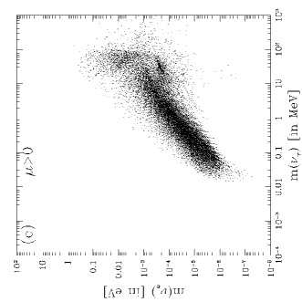
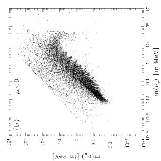
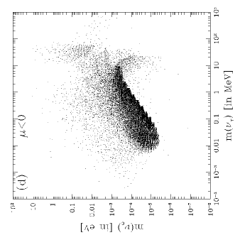
Figure 3.5: Scatter-plot of $6\times 10^{4}$ models with maximal mixing in the (a) the $m_{\nu_{\tau}}$–$m_{\nu_{\mu}}$ plane and (b) the $m_{\nu_{\tau}}$–$m_{\nu_{e}}$ plane.

3.2 Solar and atmospheric Neutrino puzzles

So far we have only considered the theoretically predicted neutrino spectrum. We have focused on the case of maximum mixing, from which the general case can be derived by rescaling the masses by appropriate powers of $\tan\theta_{i}$ ($i=1,2,3$).

Before discussing any virtue of a given model we should assure that it satisfies all experimental bounds. There are various constraints on the SUSY spectrum. In particular, from LEP-1 we know that no superpartner (except a gaugino-like neutrino) can exist with mass below $m_{\rm z}/2$[18]. Stronger constraints on strongly interacting sparticle masses are obtained from experiments at FERMILAB[18]. All of these bounds can be evaded by scaling up the soft SUSY mass parameters just like in the models with unbroken $R$-parity. Typically any model with $m_{0},m_{1/2}\mathrel{\hbox to0.0pt{\lower 3.0pt\hbox{$\mathchar 536\relax$}\hss}\raise 2.0pt\hbox{$\mathchar 318\relax$}}100~{}{\rm GeV}$ provides a sufficiently heavy sparticle spectrum. One can try to derive stronger constrains from virtual effects in processes as $b\rightarrow s\gamma$, but it requires very strong assumptions on the squark mass matrices and possible cancellations among different contributions makes it hard to derive firm bounds that are much higher than those coming from direct particle searches[26].

In order to impose the experimental constraints on the Yukawa couplings on our model we have to rewrite the Lagrangian in a basis where the Higgs fields are the only ones with non-zero VEV. In this basis, there exist $R$-parity violating Yukawa couplings proportional to the lepton masses $y_{ijk}^{F}\simeq y_{jk}^{F}v_{i}/v_{0}$ ($F=L,D$). However, they are below the experimental bounds even in the case of maximal mixing.

In principle we could now proceed to impose bounds on neutrino masses[25]

$$m_{\nu_{e}} \mathrel{\hbox to0.0pt{\lower 3.0pt\hbox{$\mathchar 536\relax$}\hss}\raise 2.0pt\hbox{$\mathchar 316\relax$}} 4.35~{}{\rm eV}\,,$$

$$m_{\nu_{\mu}} \mathrel{\hbox to0.0pt{\lower 3.0pt\hbox{$\mathchar 536\relax$}\hss}\raise 2.0pt\hbox{$\mathchar 316\relax$}} 160~{}{\rm keV}\,,$$

$$m_{\nu_{\tau}} \mathrel{\hbox to0.0pt{\lower 3.0pt\hbox{$\mathchar 536\relax$}\hss}\raise 2.0pt\hbox{$\mathchar 316\relax$}} 23~{}{\rm MeV}\,.$$ (3.7)

and lepton mixings from the partial $Z$ width[18]

$$\Gamma(Z\rightarrow e^{\pm}\mu^{\mp}) < 0.6\times 10^{-5}\,,$$

$$\Gamma(Z\rightarrow e^{\pm}\tau^{\mp}) < 1.3\times 10^{-6}\,,$$

$$\Gamma(Z\rightarrow\mu^{\pm}\tau^{\mp}) < 1.9\times 10^{-6}\,,$$ (3.8)

in order to obtain constraints on the $R$-parity breaking parameters. This route has been taken by various other authors in models with spontaneous $R$-parity breaking or in models with $R$-parity breaking Yukawa couplings[4] and very recently also in the model under investigation here[28].

However, our goal is slightly more ambitious. Rather that trying to rule out a certain region of the seven dimensional parameter space we are more interested to see whether our predictive model with only three $R$-parity violating parameters can provide the solution to actual problems. In particular, we want to find out whether the pattern of neutrino masses can provide a natural framework for a solution of the solar[16] and atmospheric[17] neutrino puzzles. The masses and mixing angles needed to solve the atmospheric neutrino puzzle are[17]

$$m_{\nu_{\tau}}^{2}-m_{\nu_{\mu}}^{2}\simeq 10^{-2}~{}{\rm eV}^{2} \,, \qquad\sin^{2}2\theta_{\mu\nu_{\tau}}\simeq 1\,.$$ (3.9)

For the solar neutrino puzzle there are three possible regions in parameter space[16],[29]

$$m_{\nu_{\mu}}^{2}-m_{\nu_{e}}^{2}\simeq 5\times 10^{-6}~{}{\rm eV}^{2} \,, \qquad\sin^{2}2\theta_{e\nu_{\mu}}\simeq 0.008$$

$$m_{\nu_{\mu}}^{2}-m_{\nu_{e}}^{2}\simeq 5\times 10^{-6}~{}{\rm eV}^{2} \,, \qquad\sin^{2}2\theta_{e\nu_{\mu}}\simeq 1$$

$$m_{\nu_{\mu}}^{2}-m_{\nu_{e}}^{2}\simeq 10^{-10}~{}{\rm eV}^{2} \,, \qquad\sin^{2}2\theta_{e\nu_{\mu}}\simeq 1\,.$$ (3.10)

The first two regions correspond to an MSW solution[30] and the third one corresponds to long-wavelength oscillations (LWO)[29]. Our analysis is similar to the one performed in ref. [5] and [13] in models with spontaneous $R$-parity breaking and in ref. [31] for models with $R$-parity breaking Yukawa couplings. The model under consideration here distinguishes itself from the later models by permitting only three $R$-parity violating parameters in addition to the usual minimal SUGRA parameters and is thus considerably more constrained. On the other hand, it does not predict any new particles below the $Z$ mass and cannot easily be tested in present[28] or future collider experiments.

The desired values of $m_{\nu_{\tau}}^{2}-m_{\nu_{\mu}}^{2}$, $\sin^{2}2\theta_{\mu\nu_{\tau}}$ and $\sin^{2}2\theta_{e\nu_{\mu}}$ can be obtained by adjusting $\tan\theta_{1}$, $\tan\theta_{2}$ and $\tan\theta_{3}$, respectively. Clearly, the desired value of $m_{\nu_{\tau}}$ [eq. 3.9] is some four to ten orders of magnitude smaller than the ones obtained for maximum $R$-parity violation [fig. 3.5] implying that $\tan\theta_{1}$ has to be rescaled by some two to five orders of magnitude. Similarly we can fix $\sin^{2}2\theta_{\mu\nu_{\tau}}$ and $\sin^{2}2\theta_{e\nu_{\mu}}$ by tuning $\tan\theta_{2}$ and $\tan\theta_{3}$. The value of $m_{\nu_{\mu}}^{2}-m_{\nu_{e}}^{2}$ is then predicted as a function of the SUSY parameters. Note that the source of the lepton number violations and lepton flavor violations are soft mixing terms that are uncorrelated with the Yukawa couplings. Thus, there is no relation between the neutrino mixing angles and the CKM-matrix of the quark sector such as in SO(10) SUSY-GUT models and we should forget any prejudice towards small mixing angles.

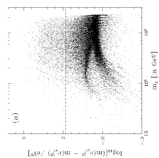
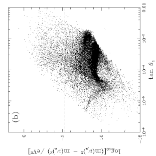
Figure 3.6: Scatter-plot of $6\times 10^{4}$ models with maximal mixing vs. (a) log${}_{10}(m_{0}/{\rm GeV})$ and (b) $\tan\theta_{1}$ for $\sin^{2}2\theta_{e\nu_{\mu}}=0.008$

We begin our numerical analysis for the case of small mixing ( i.e.  $\sin^{2}2\theta_{e\nu_{\mu}}=0.008$). In fig. 3.6 we present the prediction of $m_{\nu_{\mu}}^{2}-m_{\nu_{e}}^{2}$ obtained by scanning over the entire SUSY parameter space. The dashed line indicates the value required to solve the solar neutrino puzzle. The SUSY parameters are chosen as described in the last section. We present the prediction of $m_{\nu_{\mu}}^{2}-m_{\nu_{e}}^{2}$ as a function of (a) $m_{0}$ and (b) $\tan\theta_{1}$. The value corresponding to a MSW solution of the solar neutrino problem is indicated by a dashed line. We see that the value of $m_{\nu_{\mu}}^{2}-m_{\nu_{e}}^{2}$ is uncorrelated with $m_{0}$ and grows with $\tan\theta_{1}$. By requiring $m_{\nu_{\mu}}^{2}-m_{\nu_{e}}^{2}=5\times 10^{-6}~{}{\rm eV}^{2}$ we find that $2\times 10^{-5}\mathrel{\hbox to0.0pt{\lower 3.0pt\hbox{$\mathchar 536\relax$}\hss}\raise 2.0pt\hbox{$\mathchar 316\relax$}}\tan\theta_{1}\mathrel{\hbox to0.0pt{\lower 3.0pt\hbox{$\mathchar 536\relax$}\hss}\raise 2.0pt\hbox{$\mathchar 316\relax$}}5\times 10^{-3}$.

In fig. 3.7 we present a histogram of the number of models $N$ that yield a particular prediction for $m_{\nu_{\mu}}^{2}-m_{\nu_{e}}^{2}$. We have used the same set of models as in fig. 3.6. The dashed (dotted) line indicates the value required to solve the solar neutrino puzzle via the MSW-effect (LWO). We see that the predicted value of $m_{\nu_{\mu}}$ in most models is about one order of magnitude below the value needed to solve the solar neutrino problem (the value of $m_{\nu_{e}}$ is negligible in all models). However, the number of models that predict the right value is still so large that no particular fine-tuning is needed.

Figure 3.7: Histogram of the number of models that yield a particular prediction for $m_{\nu_{\mu}}^{2}-m_{\nu_{e}}^{2}$ and a scatter plot of all the model in the $\tan\beta$–$\tan\theta_{1}$ plane. We use the same models as in fig 3.6. The solid curve in (b) shows the upper limit on the $R$-parity violating parameter from cosmology

In fig. 3.7(b) we have singled out all the models with $3\times 10^{-6}~{}{\rm eV}^{2}<m_{\nu_{\mu}}^{2}-m_{\nu_{e}}^{2}<7\times 10^{-6}~{}{\rm eV}^{2}$. We find a clear correlation between $\tan\beta$ and $\tan\theta_{1}$ that allows to predict $\tan\theta_{1}$ to within a factor of three for a give value of $\tan\beta$ independent of the SUSY spectrum. Let us now compare the obtained value for $\tan\theta_{1}$ with experimental constraints. The most solid constraints come from collider experiments. However, they are very weak[28] and do not constrain the region in parameter space we are interested in. Stronger constraints can be obtained by requiring that the baryon asymmetry not be washed out at the electro-weak phase transition[7]. It means that at least one of the three lepton has to stay out of chemical equilibrium, ie. the lepton number violating Yukawa couplings for the electron have to satisfy

$$y^{L}_{121}={gm_{\mu}\over\sqrt{2}m_{\rm w}}{\mu_{3}\over\mu_{0}}=6\,10^{-4}{\tan\theta_{1}\sin\theta_{2}\sin\theta_{3}\over\cos\beta}\mathrel{\hbox to0.0pt{\lower 3.0pt\hbox{$\mathchar 536\relax$}\hss}\raise 2.0pt\hbox{$\mathchar 316\relax$}}10^{-7}\,,$$ (3.11)

Note that eq. 3.11 only constraints the product $\tan\theta_{1}\sin\theta_{2}\propto m_{\nu_{\tau}}\sin\theta_{2}\propto m_{\nu_{\mu}}$. In fig. 3.7(b) we see that the small mixing solution to the solar neutrino problem is compatible with eq. 3.11 (soid curve) in particular in the region of large $\tan\beta$.

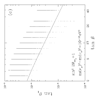
Figure 3.8: Same as in fig 3.5 except $\sin^{2}2\theta_{e\nu_{\mu}}\simeq 1$ and (b) $m_{\nu_{\mu}}^{2}-m_{\nu_{e}}^{2}=510^{-5}~{}{\rm eV}^{2}$ and (c) $m_{\nu_{\mu}}^{2}-m_{\nu_{e}}^{2}=10^{-10}~{}{\rm eV}^{2}$. Note that maximum $\nu_{e}$–$\nu_{\mu}$ mixing leads to much stronger constraints on $\tan\theta_{1}$

We will now investigate the region of large $\nu_{e}$–$\nu_{\mu}$ mixing i.e. we adjust $\tan\theta_{3}$ such that $\sin^{2}2\theta_{e\nu_{\mu}}\simeq 1$. This case yields a spectrum of squared mass differences very similar to the previous case. The result is summarized in fig. 3.8. We see that the value of $m_{\nu_{\mu}}^{2}-m_{\nu_{e}}^{2}$ needed for an LWO explanation of the solar neutrino puzzle lies very close to the maximum. It is obtained by roughly ten times as many models as the value needed for an MSW explanation. Of course it is impossible to draw any rigorous conclusion from such a scan since we have no objective way of weighing the probability for a particular set of parameters. However, in fig. 3.7(b) we see that the large mixing MSW solution is incompatible with cosmological constraints eq. 3.11 (soid curve) while for some sets of parameters the large mixing LWO solution is allowed.

3.3 LSND and hot dark matter

In the last section we answered the question whether the solar and atmospheric neutrino problems could be solved simultaneously within the frame-work of our model. However, there are several other experimental hints that indicat the existence of neutrino oscillations. Maybe the most significant result arises from $\mu$ decay at rest which requires $m_{\nu_{\mu}}^{2}-m_{\nu_{e}}^{2}\mathrel{\hbox to0.0pt{\lower 3.0pt\hbox{$\mathchar 536\relax$}\hss}\raise 2.0pt\hbox{$\mathchar 318\relax$}}0.3~{}{\rm eV}^{2}$ and $\sin^{2}2\theta_{e\nu_{\mu}}\simeq 0.004$[32]. We perform a similar scan over the parameter space as in fig. 3.7 and fig. 3.8. Note that here the solar neutrino deficiency can be explaine by $\nu_{e}$–$\nu_{\tau}$ oscillation. Thus, we fix $\tan\theta_{1}$ by tuning $m_{\nu_{\tau}}^{2}-m_{\nu_{e}}^{2}=5\times 10^{-6}~{}{\rm eV}^{2}$ $\tan\theta_{2}$ by tuning $\sin^{2}2\theta_{e\nu_{\mu}}\simeq 0.004$ and and $\tan\theta_{3}$ by tuning $\sin^{2}2\theta_{e\nu_{\tau}}\simeq 0.008$.

Figure 3.9: Histogram of the number of models that yield a particular prediction for $m_{\nu_{\mu}}^{2}-m_{\nu_{e}}^{2}$. We use the same set of parameters as in fig 3.5 except that we only consider $\tan\beta=2$ and $\tan\beta=40$. We fix $\tan\theta_{2}$ by tuning $\sin^{2}2\theta_{e\nu_{\mu}}\simeq 0.004$ and $\tan\theta_{3}$ by tuning $\sin^{2}2\theta_{e\nu_{\tau}}\simeq 0.008$

Our result is summarized in fig. 3.9. The dotted curve shows the lower limit on $m_{\nu_{\mu}}^{2}-m_{\nu_{e}}^{2}$ compatible with the LSND result. The short dashed curve shows the upper limit on $m_{\nu_{\mu}}$ from collider experiments[18] while the long dashed curve shows the upper limit on the heavies neutrino mass from requiring that the neutrino relic density does not overclose the universe[27]. We see that for large values of $\tan\beta$ there are a few sets of parameters that can simultaneously explain the solar neutrino deficiency and the LSND result. However, since in this scenario $m_{\nu_{\mu}}$ is quite large in comparison with $m_{\nu_{\tau}}$ in the case of the atmospheric neutrino puzzle it is clear that the $R$-parity violating parameter is larger than its cosmological upper limit [7].

One of the disadvantages of models with broken $R$-parity is the instability of the lightest supersymmetric particle which cannot serve as a cold dark matter candidate. One the other hand, it has been suggested that the existence of hot dark matter (HDM) consisting of massive neutrinos with a sum of all the masses of about $7$ eV would be desirable[33]. Clearly, this condition is only compatible with both a solution to solar and atmospheric neutrino puzzle if all three neutrinos are almost mass-degenerate. This is incompatible with the hierarchical spectrum of our model (ie. $m_{\nu_{e}}\ll m_{\nu_{\mu}},m_{\nu_{\tau}}$). However, it is clearly possible to solve the solar neutrino puzzle via $\nu_{e}$–$\nu_{\mu}$ oscillation while fixing $m_{\nu_{\tau}}=7~{}{\rm eV}$. E.g, take all the models from fig. 3.7(b) and fig. 3.8(b)-(c) and replace $\tan\theta_{1}\rightarrow(7~{}{\rm eV}/0.1~{}{\rm eV})^{1/2}\tan\theta_{1}$ and $\tan\theta_{2}\rightarrow(7~{}{\rm eV}/0.1~{}{\rm eV})^{-1/2}\tan\theta_{2}$. This rescaling only changes the value of $m_{\nu_{\tau}}$ while the values of $m_{\nu_{\mu}}$, $m_{\nu_{e}}$ and the $R$-parity violating coupling constrained by eq. 3.11 remain the same.

Chapter 4 Conclusions

We have investigated the spectrum of neutrino masses and mixing angles in the MSSM with broken $R$-parity. We have focused on the model where $R$-parity breaking arises explicitly from dimension 2 terms in the superpotential. This model is characterized by only three additional parameters and can be embedded in SUSY GUT model without any constraints from the proton life-time. In this model, the $R$-parity breaking is characterized by $\tan\theta_{1}$, the $\mu$–$\tau$ mixing by $\tan\theta_{2}$, and the $e$–$\mu$ mixing by $\tan\theta_{3}$. By adjusting these parameters we can solve the solar and atmospheric neutrino puzzles without fine-tuning. In particular, we have shown that a large hierarchy $m_{\nu_{\tau}}\gg m_{\nu_{\mu}}\gg m_{\nu_{e}}$ is quite natural even in the case of maximum mixing and may favor a LWO explanation of the solar neutrino puzzle. To obtain the correct neutrino masses we need $\tan\theta_{1}\simeq 10^{-x}$ ($x=2\sim 5$; this ratio may be explained as the ratio of $M_{\rm GUT}/M_{\rm P}$) but no additional particles and no new intermediate scale. Requiring that the baryon asymmetry not be washed out at the electro-weak phase transition rules out the large mixing MSW solution, while some regions of the LWO solution and small mixing MSW solution are allowed.

Finally, we demonstrate that there are regions in parameter space where the solution to the solar neutrino puzzle is compatible with either the LSND result or the existence of a $7~{}{\rm eV}$ HDM neutrino.

Acknowledgement: I would like to thank D. Pierce for comparison of the numerical results, S. Davidson, G. Raffelt and N. Polonsky for many useful and pleasant conversations and the ITP in Santa Barbara where this work was completed for their kind hospitality.

This work was supported in parts by the National Science Foundation Grant No. PHY94-07194.

Appendix A The RGEs for the $R$-parity violating terms

Here we present the RGEs for the $R$ symmetry breaking terms. They can easily be derived from ref. [34] In our model without $R$-parity violating Yukawa couplings and with diagonal lepton Yukawa couplings the RGEs for $\mu_{I}$ reduce to

$$32\pi^{2}{{\rm d}\mu_{0}\over{\rm d}t} = \mu_{0}\left({\rm tr\,}y^{L2}+N_{c}{\rm tr\,}y^{D2}+N_{c}{\rm tr\,}y^{U2}-3g^{2}-g^{\prime 2}\right)\,,$$

$$32\pi^{2}{{\rm d}\mu_{i}\over{\rm d}t} = \mu_{i}\left(y^{L}_{(ii)}y^{L}_{(ii)}+N_{c}{\rm tr\,}y^{U2}-3g^{2}-g^{\prime 2}\right)\,,$$ (A.1)

where we do not sum over indices in brackets. Furthermore, for our purposes it is more convenient to write $B_{I}^{\mu}=B_{IJ}\mu_{J}$ with

$$16\pi^{2}{{\rm d}B_{00}\over{\rm d}t} = {\rm tr\,}A^{L}y^{L}+N_{c}{\rm tr\,}A^{D}y^{D}+N_{c}{\rm tr\,}A^{U}y^{U}+3Mg^{2}+M^{\prime}g^{\prime 2}\,,$$

$$16\pi^{2}{{\rm d}B_{(ii)}\over{\rm d}t} = A^{L}_{(ii)}y^{L}_{(ii)}+N_{c}{\rm tr\,}A^{U}y^{U}+3Mg^{2}+M^{\prime}g^{\prime 2}\,,$$ (A.2)

Appendix B The mass at tree-level

In our model the electro-weak symmetry is broken via a the vacuum expectation value (VEV) of the neutral CP-even Higgs boson fields and the sneutrino fields, $\bar{v}\equiv{\langle H\rangle}$ and $v_{I}\equiv{\langle L_{I}\rangle}$. We find it convenient to present all the masses and interactions in the basis where the interactions are $R$-parity conserving and $R$-parity breaking is only parameterized by the mass parameters $\mu_{i}$, $B^{\mu}_{i}$, and after electroweak symmetry breaking also by $v_{i}$. Furthermore, it is convenient to define the unit vector $u_{I}\equiv v_{I}/v$.

$$\begin{array}[]{|c||c|c|c|c|c|c|}\hline\cr\Phi&Q&U&D&L&E&H\\ \hline\cr\hline\cr Y_{\Phi}&{1\over 3}&{4\over 3}&-{2\over 3}&-1&-2&1\\ \hline\cr\end{array}$$

Table B.1: The hypercharges of the Higgs fields and the matter fields. Note that $Y_{\Phi^{c}}=-Y_{\Phi}$ for $\Phi=U,D,E$

In our notation we use calligraphic letters to denote the mass matrices and interaction matrices in the electro-weak basis and roman letters for the mass matrices and interaction matrices in the basis of the mass eigenstates. The hypercharges are listed in table B.1.

In models with broken $R$-parity the neutrinos mix with the neutralinos. We can write the potential as

$$V={\textstyle{1\over 2}}\left(\matrix{\psi^{0}}\right){\cal M}_{\chi^{0}}\left(\matrix{\psi^{0}}\right)^{T}+{\rm H.c.}\,,$$ (B.1)

where $\psi^{0}_{n}=\left(-i\lambda^{\prime},-i\lambda^{3},\psi_{H}^{2},\psi_{L_{I}}^{1}\right)$ and the $7\times 7$ neutrino/neutralino mass matrix

$${\cal M}_{\chi^{0}}=\left(\matrix{M^{\prime}&0&m_{\rm z}s_{\rm w}s_{\beta}&-m_{\rm z}s_{\rm w}c_{\beta}u_{I}\cr{}&M&-m_{\rm z}c_{\rm w}s_{\beta}&m_{\rm z}c_{\rm w}c_{\beta}u_{I}\cr{}&{}&0&-\mu_{I}\cr{}&{\rm symmetric}&{}&0\cr}\right)\,.$$ (B.2)

where we have defined $c_{\rm w}\equiv\cos\theta_{\rm w}\equiv m_{\rm w}/m_{\rm z}$ and $\tan\beta\equiv\bar{v}/v$, $s_{\beta}\equiv\sin\beta$, etc. We now define the unitary matrix $Z$ such that the matrix $m_{\chi^{0}}=Z^{*}{\cal M}_{\chi^{0}}Z^{-1}$ is diagonal and the value of the diagonal elements is ordered by magnitude.

The mass matrix in eq. B.2 still has two massless eigenstates corresponding to two neutrinos. However, one neutrino acquires a mass

$$m_{\nu_{3}}\simeq{c_{\beta}^{2}\left(Ms_{\rm w}^{2}+M^{\prime}c_{\rm w}^{2}\right)m_{\rm z}^{2}\mu^{2}\sin^{2}(\theta_{1}-\theta_{1}^{\prime})\over M^{\prime}M\mu_{0}^{2}-2s_{\beta}c_{\beta}\left(Ms_{\rm w}^{2}+M^{\prime}c_{\rm w}^{2}\right)m_{\rm z}^{2}\mu_{0}}\,,$$ (B.3)

at tree-level. Furthermore, the charged leptons mix with the charginos. In complete analogy to the MSSM we can write

$$\psi^{+} = \left(-i\lambda^{+},\psi_{H}^{1},\psi_{E^{c}_{i}}\right)$$

$$\psi^{-} = \left(-i\lambda^{-},\psi_{L_{I}}^{2}\right)$$ (B.4)

The potential is given by

$$V=\psi^{-}{\cal M}_{\chi^{\pm}}\psi^{+}+\rm H.c.$$ (B.5)

The $5\times 5$ mass matrix is given by

$${\cal M}_{\chi^{\pm}}=\left(\matrix{M&\sqrt{2}m_{\rm w}\sin\beta&0\cr\sqrt{2}m_{\rm w}\cos\beta u_{0}&\mu_{0}&-y^{L}_{ij}v_{i}\cr\sqrt{2}m_{\rm w}\cos\beta u_{i}&\mu_{i}&y^{L}_{ij}v_{0}\cr}\right)\,,$$ (B.6)

We now define the unitary matrices $U^{R}$, $U^{L}$ such that $m_{\chi^{\pm}}\equiv U^{R*}{\cal M}_{\chi^{\pm}}(U^{L})^{-1}$ is diagonal (in the MSSM $U^{R}=U$ and $U^{L}=V$). Then we can write the chargino mass eigenstates as four component spinors

$$\chi^{+}=\left(\matrix{U^{L}\psi^{+}\cr U^{R}\overline{\psi}^{-}}\right)\,,$$ (B.7)

Let us consider the Higgs sector. In the case of explicitly broken $R$-parity (i.e. $\mu_{i}\neq 0$) we find that the Higgs multiplets mix with the lepton multiplets. In particular, the sneutrinos acquire a non-zero VEV. The system of five equation corresponding to the minimum conditions of these fields can be solved most easily numerically by iteration. The tree-level mass matrix of the neutral, CP-even Higgs/slepton mass matrix is given by

$${\cal M}_{H^{0}}=\left(\matrix{\mu_{I}^{2}+m_{H}^{2}+{\textstyle{1\over 2}}m_{\rm z}^{2}(3s_{\beta}^{2}-c_{\beta}^{2})&-B_{J}^{\mu}-m_{\rm z}^{2}s_{\beta}c_{\beta}u_{J}\cr-B_{I}^{\mu}-m_{\rm z}^{2}s_{\beta}c_{\beta}u_{I}&\mu_{I}\mu_{J}+m_{L_{IJ}}^{2}+{\textstyle{1\over 2}}m_{\rm z}^{2}[c_{\beta}^{2}(2u_{I}u_{J}+\delta_{IJ})-s_{\beta}^{2}\delta_{IJ}]}\right)\,,$$ (B.8)

and tree-level mass matrix of the neutral, CP-odd Higgs/slepton mass matrix is given by

$${\cal M}_{A^{0}} = \left(\matrix{\mu_{I}^{2}+m_{H}^{2}+{\textstyle{1\over 2}}m_{\rm z}^{2}(s_{\beta}^{2}-c_{\beta}^{2})&-B_{J}^{\mu}\cr-B_{I}^{\mu}&\mu_{I}\mu_{J}+m_{L_{IJ}}^{2}+{\textstyle{1\over 2}}m_{\rm z}^{2}(c_{\beta}^{2}-s_{\beta}^{2})\delta_{IJ}}\right)$$ (B.9)

$$+\xi_{\rm z}m_{\rm z}^{2}\left(\matrix{\sin^{2}\beta&\sin\beta\cos\beta u_{J}\cr\sin\beta\cos\beta u_{I}&\cos^{2}\beta u_{I}u_{J}}\right)\,,$$

Finally, the two charged Higgs bosons mix with the charged sleptons. The mass matrix in the electro-weak eigenbasis $H_{a}^{+}=(H^{+},\widetilde{E}^{L+}_{I},\widetilde{E}^{R+}_{i})$ with $a=1,...,8$ becomes

$${\cal M}_{H^{\pm}}^{2}=\left(\matrix{{\cal M}_{LL}^{2}&{\cal M}_{LR}^{2}\cr{\cal M}_{RL}^{2}&{\cal M}_{RR}^{2}}\right)\,,$$ (B.10)

where $\widetilde{E}^{L+}=(\widetilde{L}^{-})^{*}$, $\widetilde{E}^{R+}=\widetilde{E}^{c}$ where the submatrices are given by

$${\cal M}_{LL}^{2} = \left(\matrix{M_{H}^{2}+\mu^{2}&-B^{\mu}_{J}\cr-B^{\mu}_{I}&M_{L_{IJ}}^{2}+\mu_{I}\mu_{J}+M_{IJ}^{y2}}\right)-{\textstyle{1\over 2}}m_{\rm z}^{2}s_{\rm w}^{2}\cos 2\beta\left(\matrix{Y_{H}&0\cr 0&Y_{L}\delta_{IJ}}\right)$$ (B.11)

$$+{\textstyle{1\over 2}}m_{\rm w}^{2}\left(\matrix{1&-\sin 2\beta u_{J}\cr-\sin 2\beta u_{I}&2\cos^{2}\beta u_{I}u_{J}-\cos 2\beta\delta_{IJ}}\right)$$

$$+\xi_{\rm w}m_{\rm w}^{2}\left(\matrix{\sin^{2}\beta&\sin\beta\cos\beta u_{J}\cr\sin\beta\cos\beta u_{I}&\cos^{2}\beta u_{I}u_{J}}\right)$$

with $M_{IJ}^{y2}$ given by

$$M_{00}^{y2} = M_{0j}^{y2}=M_{i0}^{y2}=0\,,$$

$$M_{ij}^{y2} = y^{L}_{ik}y^{L}_{jk}v_{0}^{2}+y^{L}_{ik}y^{L}_{jl}v_{k}v_{l}\,,$$ (B.12)

and

$${\cal M}_{LR}^{2}=\left(\matrix{y_{ij}^{L}(v_{0}\mu_{i}-v_{i}\mu_{0})\cr A_{ij}^{L}v_{i}-\mu_{i}y_{ij}^{L}\overline{v}\cr-A_{ij}^{L}v_{0}+\mu_{0}y_{ij}^{L}\overline{v}}\right)$$ (B.13)

$${\cal M}_{RR}^{2}=M_{E_{ij}}^{2}-{\textstyle{1\over 2}}Y_{E^{c}}m_{\rm z}^{2}s_{\rm w}^{2}\cos 2\beta+y^{L}_{ki}y^{L}_{kj}v_{0}^{2}+y^{L}_{ki}y^{L}_{lj}v_{k}v_{l}$$ (B.14)

Note that the gauge dependent pieces arise from the gauge fixing terms in the $R_{\xi}$ gauge. They give masses to the goldstone-bosons $m_{A^{0}_{1}}^{2}=\xi_{\rm z}m_{\rm z}^{2}$ and $m_{H^{\pm}_{1}}^{2}=\xi_{\rm w}m_{\rm w}^{2}$, respectively, Inside our one-loop calculation of Appendix D these unphysical fields are treaded just like the physical fields.

Appendix C Vertices

In the following appendix we summarize a set of vertices in a notation that is convenient for SUSY theories with broken $R$ parity[[28],[21]]. Note, that due to the minus signs in eq. 2.6 the fields $\psi_{x}^{-}$ defined in eq. B.4 are minus the fermionic partners of $H_{x}^{-}$ ($x=2,3,4,5$) defined above eq. B.10.

The Feynman rules are given by $i\gamma_{\mu}(V^{L}L+V^{R}R)$, $-i(V^{L}L+V^{R}R)$, $-(V^{L}L+V^{R}R)$, for couplings of a fermion pair to a gauge boson, a complex or CP-even scalar, and a CP-odd scalar, respectively (here, $V^{L}$ and $V^{R}$ is the generic notation for all the vertices listed below. Note that we have included the gauge coupling constant in the definitions of $V^{L/R}$).

The $W^{-}\chi^{0}_{n}\chi^{+}_{x}$ vertices are given by ($n=1,..,7$ and $x=1,..,5$)

$${\cal O}^{L}_{nx} = g\left(\delta_{n2}\delta_{x1}-{1\over\sqrt{2}}\delta_{n3}\delta_{x2}\right)\,,$$

$${\cal O}^{R}_{nx} = g\left(\delta_{n2}\delta_{x1}+{1\over\sqrt{2}}\sum_{\alpha=2}^{5}\delta_{n\alpha+2}\delta_{x\alpha}\right)\,.$$ (C.1)

The $Z\chi^{-}_{x}\chi^{+}_{y}$ vertices are given by

$${\cal O}^{\prime L} = {g\over 2c_{\rm w}}\rm diag\left(2s_{\rm w}^{2}-2,2s_{\rm w}^{2}-1,2s_{\rm w}^{2}\delta_{(ii)}\right)\,,$$

$${\cal O}^{\prime R} = {g\over 2c_{\rm w}}\rm diag\left(2s_{\rm w}^{2}-2,(2s_{\rm w}^{2}-1)\delta_{(II)}\right)\,,$$ (C.2)

no summation over indices in parenthesis. The $Z\chi^{0}_{m}\chi^{0}_{n}$ vertices are given by

$${\cal O}^{\prime\prime L} = {g\over 2c_{\rm w}}\rm diag\left(0,0,1,-\delta_{(II)}\right)\,,$$

$${\cal O}^{\prime\prime R} = -{\cal O}^{\prime\prime L}$$ (C.3)

The $H^{0}_{x}\chi^{-}_{y}\chi^{+}_{z}$ vertices are given by

$${\cal Q}^{L}_{xyz}={1\over\sqrt{2}}\times\cases{g\delta_{1y}\delta_{z2}&for $x=1$\cr g\delta_{2y}\delta_{z1}+y^{E}_{y-2z-2}&for $x=2$\cr g\delta_{xy}\delta_{z1}-y^{E}_{x-2z-2}\delta_{y2}&for $x=3,4,5,$}$$ (C.4)

and ${\cal Q}^{R}_{xyz}={\cal Q}^{L}_{xzy}$. The $A^{0}_{x}\chi^{-}_{y}\chi^{+}_{z}$ vertices are given by

$${\cal S}^{L}_{xyz}=\cases{{\cal Q}^{L}_{xyz}&for $x=1$\cr-{\cal Q}^{L}_{xyz}&for $x=2,3,4,5,$}$$ (C.5)

and ${\cal S}^{R}_{xyz}=-{\cal S}^{L}_{xzy}$. The $H^{0}_{x}\chi^{0}_{m}\chi^{0}_{n}$ vertices are given by

$${\cal Q}^{\prime\prime P}_{xmn}=\cases{-{g\over 2}\left[\delta_{mx+2}\left(\delta_{n2}-\tan\theta_{\rm w}\delta_{n1}\right)+\delta_{nx+2}\left(\delta_{m2}-\tan\theta_{\rm w}\delta_{m1}\right)\right]&for $x=1$\cr{g\over 2}\left[\delta_{mx+2}\left(\delta_{n2}-\tan\theta_{\rm w}\delta_{n1}\right)+\delta_{nx+2}\left(\delta_{m2}-\tan\theta_{\rm w}\delta_{m1}\right)\right]&for $x=2,3,4,5$}$$ (C.6)

where $P=L,R$. The $A^{0}_{x}\chi^{0}_{m}\chi^{0}_{n}$ vertices are given by

$${\cal S}^{\prime\prime L}_{xmn}=-{\cal S}^{\prime\prime R}_{xmn}={g\over 2}\left[\delta_{mx+2}\left(\delta_{n2}-\tan\theta_{\rm w}\delta_{n1}\right)+\delta_{nx+2}\left(\delta_{m2}-\tan\theta_{\rm w}\delta_{m1}\right)\right]\,,$$ (C.7)

The $H^{-}_{a}\chi^{0}_{n}\chi^{+}_{x}$ vertices are given by

$${\cal Q}^{\prime L}_{anx}=\cases{Y_{H}{g^{\prime}\over\sqrt{2}}\delta_{n1}\delta_{x2}+{g\over\sqrt{2}}\delta_{n2}\delta_{x2}+g\delta_{n3}\delta_{x1}&for $a=1$\cr y_{n-4x-2}^{L}&for $a=2$\cr-y_{a-2x-2}^{L}\delta_{n4}&for $a=3,4,5$\cr Y_{E}{g^{\prime}\over\sqrt{2}}\delta_{n1}\delta_{xa-3}&for $a=6,7,8$}$$ (C.8)

$${\cal Q}^{\prime R}_{anx} = \cases{0&for $a=1$\cr-Y_{L}{g^{\prime}\over\sqrt{2}}\delta_{n1}\delta_{xa}+{g\over\sqrt{2}}\delta_{n2}\delta_{xa}-g\delta_{na+2}\delta_{x1}&for $a=2,..,5$\cr-y_{n-4a-5}^{L}\delta_{x2}+y_{x-2a-5}^{L}\delta_{n4}&for $a=6,7,8$}$$ (C.9)

The $\tilde{u}_{\alpha}\bar{u}_{b}\chi_{n}^{0}$ vertex is

$${\cal V}_{\alpha bn}^{uL} = y^{U}_{\alpha b}\delta_{n3}-{1\over\sqrt{2}}Y_{U}g^{\prime}\delta_{\alpha-3b}\delta_{n1}$$

$${\cal V}_{\alpha bn}^{uR} = y^{U}_{b\alpha-3}\delta_{n3}+{1\over\sqrt{2}}g\delta_{\alpha b}\delta_{n2}+{1\over\sqrt{2}}Y_{Q}g^{\prime}\delta_{\alpha b}\delta_{n1}$$ (C.10)

The $\tilde{d}_{\alpha}\bar{d}_{b}\chi_{n}^{0}$ vertex is

$${\cal V}_{\alpha bn}^{dL} = y^{D}_{\alpha b}\delta_{n4}-{1\over\sqrt{2}}Y_{D}g^{\prime}\delta_{\alpha-3b}\delta_{n1}$$

$${\cal V}_{\alpha bn}^{dR} = y^{D}_{b\alpha-3}\delta_{n4}-{1\over\sqrt{2}}g\delta_{\alpha b}\delta_{n2}+{1\over\sqrt{2}}Y_{Q}g^{\prime}\delta_{\alpha b}\delta_{n1}$$ (C.11)

The $\tilde{u}_{\alpha}\bar{d}_{b}\chi_{x}^{-}$ vertex is

$${\cal V}_{\alpha bx}^{\tilde{u}L}C = -y^{D}_{\alpha b}\delta_{x2}C$$

$${\cal V}_{\alpha bx}^{\tilde{u}R}C = \left(g\delta_{\alpha b}\delta_{x1}-y^{U}_{b\alpha-3}\delta_{x2}\right)C$$ (C.12)

The $\tilde{d}_{\alpha}\bar{u}_{b}\chi_{x}^{+}$ vertex is

$${\cal V}_{\alpha bx}^{\tilde{d}L} = -y^{U}_{\alpha b}\delta_{x2}$$

$${\cal V}_{\alpha bx}^{\tilde{d}R} = g\delta_{\alpha b}\delta_{x1}-y^{D}_{b\alpha-3}\delta_{x2}$$ (C.13)

Definition and more details on the charge conjugation operator $C$ can be found in ref. [36].

The vertices in the mass eigenbasis are given by

$$O_{nx}^{P} = Z_{n\tilde{n}}U^{P}_{x\tilde{x}}{\cal O}_{\tilde{n}\tilde{x}}^{P}$$

$$O_{xy}^{\prime P} = U^{P}_{x\tilde{x}}U^{P}_{y\tilde{y}}{\cal O}_{\tilde{x}\tilde{y}}^{\prime P}$$

$$O_{mn}^{\prime\prime P} = Z_{m\tilde{m}}Z_{n\tilde{n}}{\cal O}_{\tilde{m}\tilde{n}}^{\prime\prime P}$$

$$S_{xyz}^{L} = U^{A^{0}}_{x\tilde{x}}U^{R}_{y\tilde{y}}U^{L}_{z\tilde{z}}{\cal S}_{\tilde{x}\tilde{y}\tilde{z}}^{L}$$

$$S_{xyz}^{R} = U^{A^{0}}_{x\tilde{x}}U^{L}_{y\tilde{y}}U^{R}_{z\tilde{z}}{\cal S}_{\tilde{x}\tilde{y}\tilde{z}}^{R}$$

$$Q_{xyz}^{L} = U^{H^{0}}_{x\tilde{x}}U^{R}_{y\tilde{y}}U^{L}_{z\tilde{z}}{\cal Q}_{\tilde{x}\tilde{y}\tilde{z}}^{L}$$

$$Q_{xyz}^{R} = U^{H^{0}}_{x\tilde{x}}U^{L}_{y\tilde{y}}U^{R}_{z\tilde{z}}{\cal Q}_{\tilde{x}\tilde{y}\tilde{z}}^{R}$$

$$Q_{\alpha nx}^{\prime P} = U^{H^{\pm}}_{\alpha\tilde{\alpha}}Z_{n\tilde{n}}U^{P}_{x\tilde{x}}{\cal Q}_{\tilde{\alpha}\tilde{n}\tilde{x}}^{\prime P}$$

$$Q_{xmn}^{\prime\prime P} = U^{H^{0}}_{x\tilde{x}}Z_{m\tilde{m}}Z_{n\tilde{n}}{\cal Q}_{\tilde{x}\tilde{m}\tilde{n}}^{\prime\prime P}$$

$$S_{xmn}^{\prime\prime P} = U^{A^{0}}_{x\tilde{x}}Z_{m\tilde{m}}Z_{n\tilde{n}}{\cal S}_{\tilde{x}\tilde{m}\tilde{n}}^{\prime\prime P}$$

$$V_{\alpha ax}^{\tilde{d}P} = U^{\tilde{d}}_{\alpha\tilde{\alpha}}U_{x\tilde{x}}^{P}{\cal V}_{\tilde{\alpha}a\tilde{x}}^{\tilde{d}P}$$

$$V_{\alpha ax}^{\tilde{u}L/R} = U^{\tilde{u}}_{\alpha\tilde{\alpha}}U_{x\tilde{x}}^{R/L}{\cal V}_{\tilde{\alpha}a\tilde{x}}^{\tilde{u}L/R}$$

$$V_{\alpha am}^{qP} = U^{\tilde{q}}_{\alpha\tilde{\alpha}}Z_{m\tilde{m}}{\cal V}_{\tilde{\alpha}a\tilde{m}}^{qP}\qquad(q=u,d)\,,$$ (C.14)

for $P=L,R$ (here $U^{L}\equiv V$, and $U^{R}\equiv U$). Furthermore, we have assumed that the Yukawa matrices $y^{U/D/L}$ are diagonal. The unitary matrices $U^{\tilde{q}}$ diagonalizing the squark mass matrices are defined analogous to eq. 2.15.

Appendix D The One-Loop Corrected Neutrino/Neutralino
Mass Matrix

In this appendix we present the complete one-loop radiative corrections to the full neutrino/neutralino mass matrix. Note that for the radiative generation of the neutrino masses only the diagrams involving Higgs fields are relevant. We have regularized the divergences by dimensional reduction[23]. The calculation has been done in the t’Hooft–Feynman gauge ($\xi=1$). Note that the self-energy diagrams and as a consequence also the running $\overline{\rm DR}$ masses as defined in eq. 3.1 are gauge-dependent. There are seven types of diagrams contributing to the self-energy of the Neutrino/Neutralino: charged Higgs/chargino, CP-even Higgs/neutralino, CP-odd Higgs/neutralino, up quark/squark, down quark/squark, $W^{\pm}$/chargino, $Z$/neutralino. Their results are

$$\Sigma^{V}_{nm} = {\textstyle{1\over 2}}\left(\Sigma^{R}_{nm}+\Sigma^{L}_{nm}\right)$$ (D.1)

$$= -{1\over 16\pi^{2}}\left[\sum_{a,x}\left(Q^{\prime L}_{anx}Q^{\prime L}_{amx}+Q^{\prime R}_{anx}Q^{\prime R}_{amx}\right)B_{1}(p^{2},m_{\chi^{\pm}_{x}}^{2},m_{H^{\pm}_{a}}^{2})\right.$$

$$+{\textstyle{1\over 2}}\sum_{x,k}\left(Q^{\prime\prime L}_{xnk}Q^{\prime\prime L}_{xmk}+Q^{\prime\prime R}_{xnk}Q^{\prime\prime R}_{xmk}\right)B_{1}(p^{2},m_{\chi^{0}_{k}}^{2},m_{H^{0}_{x}}^{2})$$

$$+{\textstyle{1\over 2}}\sum_{x,k}\left(S^{\prime\prime L}_{xnk}S^{\prime\prime L}_{xmk}+S^{\prime\prime R}_{xnk}S^{\prime\prime R}_{xmk}\right)B_{1}(p^{2},m_{\chi^{0}_{k}}^{2},m_{A^{0}_{x}}^{2})$$

$$+3\sum_{\alpha,b}\left(V^{uL}_{\alpha bn}V^{uL}_{\alpha bm}+V^{uR}_{\alpha bn}V^{uR}_{\alpha bm}\right)B_{1}(p^{2},m_{u_{b}}^{2},m_{\tilde{u}_{\alpha}}^{2})$$

$$+3\sum_{\alpha,b}\left(V^{dL}_{\alpha bn}V^{dL}_{\alpha bm}+V^{dR}_{\alpha bn}V^{dR}_{\alpha bm}\right)B_{1}(p^{2},m_{d_{b}}^{2},m_{\tilde{d}_{\alpha}}^{2})$$

$$+2\sum_{x}\left(O^{L}_{nx}O^{L}_{mx}+O^{R}_{nx}O^{R}_{mx}\right)B_{1}(p^{2},m_{\chi^{\pm}_{x}}^{2},m_{\rm w}^{2})$$

$$\left.+\sum_{k}\left(O^{\prime\prime L}_{nk}O^{\prime\prime L}_{mk}+O^{\prime\prime R}_{nk}O^{\prime\prime R}_{mk}\right)B_{1}(p^{2},m_{\chi^{0}_{k}}^{2},m_{\rm z}^{2})\right]\,,$$

$$\Pi^{V}_{nm} = {\textstyle{1\over 2}}\left(\Pi_{nm}^{R}+\Pi^{L}_{nm}\right)$$ (D.2)

$$= -{1\over 16\pi^{2}}\left[\sum_{a,x}m_{\chi^{\pm}_{x}}\left(Q^{\prime L}_{anx}Q^{\prime R}_{amx}+Q^{\prime R}_{anx}Q^{\prime L}_{amx}\right)B_{0}(p^{2},m_{\chi^{\pm}_{x}}^{2},m_{H^{\pm}_{a}}^{2})\right.$$

$$+{\textstyle{1\over 2}}\sum_{x,k}m_{\chi^{0}_{k}}\left(Q^{\prime\prime L}_{xnk}Q^{\prime\prime R}_{xmk}+Q^{\prime\prime R}_{xnk}Q^{\prime\prime L}_{xmk}\right)B_{0}(p^{2},m_{\chi^{0}_{k}}^{2},m_{H^{0}_{x}}^{2})$$

$$+{\textstyle{1\over 2}}\sum_{x,k}m_{\chi^{0}_{k}}\left(S^{\prime\prime L}_{xnk}S^{\prime\prime R}_{xmk}+S^{\prime\prime R}_{xnk}S^{\prime\prime L}_{xmk}\right)B_{0}(p^{2},m_{\chi^{0}_{k}}^{2},m_{A^{0}_{x}}^{2})$$

$$+3\sum_{\alpha,b}m_{u_{b}}\left(V^{uL}_{\alpha bn}V^{uR}_{\alpha bm}+V^{uR}_{\alpha bn}V^{uL}_{\alpha bm}\right)B_{0}(p^{2},m_{u_{b}}^{2},m_{\tilde{u}_{\alpha}}^{2})$$

$$+3\sum_{\alpha,b}m_{d_{b}}\left(V^{dL}_{\alpha bn}V^{dR}_{\alpha bm}+V^{dR}_{\alpha bn}V^{dL}_{\alpha bm}\right)B_{0}(p^{2},m_{d_{b}}^{2},m_{\tilde{d}_{\alpha}}^{2})$$

$$-4\sum_{x}m_{\chi^{\pm}_{x}}\left(O^{L}_{nx}O^{R}_{mx}+O^{R}_{nx}O^{L}_{mx}\right)B_{0}(p^{2},m_{\chi^{\pm}_{x}}^{2},m_{\rm w}^{2})$$

$$\left.-2\sum_{k}m_{\chi^{0}_{k}}\left(O^{\prime\prime L}_{nk}O^{\prime\prime R}_{mk}+O^{\prime\prime R}_{nk}O^{\prime\prime L}_{mk}\right)B_{0}(p^{2},m_{\chi^{0}_{k}}^{2},m_{\rm z}^{2})\right]\,.$$

The $B_{0}$ and $B_{1}$ functions are defined by

$$[B_{0}(q^{2},m_{1}^{2},m_{2}^{2}),q_{\mu}B_{1}(q^{2},m_{1}^{2},m_{2}^{2})]=-16\,i\pi^{2}\int{{\rm d}^{n}k\over(2\pi)^{n}}{[1,k_{\mu}]\over D}\,,$$ (D.3)

where $D\equiv(k^{2}-m_{1}^{2}+i\delta)[(k+q)^{2}-m_{2}^{2}+i\delta]$.

Bibliography

[1] See, for example, L. Susskind,
Phys. Rep.104, 1881 (1984).
[2]
for a review, see, e.g. , H.P. Nilles, Phys. Rep.110, 1 (1984);
H.E. Haber and G.L. Kane, Phys. Rep.117, 75 (1985);
R. Barbieri, Riv. Nuovo Cimento 11, 1 (1988).
[3]
H. Dreiner and G.G. Ross, Nucl. Phys.B365, 597 (1991);
H. Dreiner and R.J.N. Phillips, Nucl. Phys.B367, 591 (1991);
J. Butterworth and H. Dreiner, Nucl. Phys.B397, 3 (1993);
C.E. Carlson, P. Roy and M. Sher, Phys. Lett.B357, 99 (1995);
G. Bhattacharyya, D. Choudhury and K. Sridhar, Phys. Lett.B355, 193 (1995).
[4]
K. Enqvist, A. Masiero and A. Riotto, Nucl. Phys.B373, 95 (1992).
[5]
J.C. Romao and J.W.F. Valle, Nucl. Phys.B381, 87 (1992)
I. Umemura and K. Yamamoto, Nucl. Phys.B423, 405 (1994).
[6]
C.E. Carlson, P. Roy and M. Sher, Phys. Lett.B357, 99 (1995).
[7]
B.A. Campbell, S. Davidson,
J. Ellis and K.A. Olive, Phys. Lett.B256, 457 (1991);
H. Dreiner and G.G. Ross, Nucl. Phys.B410, 88 (1993).
[8] A.Yu Smirnov and F. Vissani, Nucl. Phys.B460, 37 (1996).
[9]
N. Sakai and T. Yanagida, Nucl. Phys.B197, 533 (1982).
[10] J. Ellis, J.S. Hagelin, D.V. Dimopoulos, K.A. Olive and
M. Srednicki, Nucl. Phys.B238, 453 (1984).
[11] L.J. Hall and M. Suzuki, Nucl. Phys.B231, 419 (1984).
[12]
A. Santamaria and J.W.F. Valle, Phys. Lett.B195, 423 (1987);
Phys. Rev. Lett.60, 397 (1988); Phys. Rev.D39, 1780 (1989).
[13]
A. Masiero and J.W.F. Valle, Phys. Lett.B251, 142 (1990);
V. Berezinsky, A. Masiero and J.W.F. Valle, Phys. Lett.B266, 382 (1991).
[14]
J.E. Kim and H.P. Nilles, Phys. Lett.B138, 150 (1984);
G.F. Giudice and A. Masiero, Phys. Lett.B206, 480 (1988)
E.J. Chun, J.E. Kim and H.P. Nilles, Nucl. Phys.B370, 105 (1992);
J.A. Casas and C. Muñoz, Phys. Lett.B306, 288 (1993);
R. Hempfling, Phys. Lett.B329, 222 (1994).
[15] S. Dimopoulos and H. Georgi,
Nucl. Phys. B193, 150 (1981).
[16]
R. Davis et al., Phys. Rev. Lett.20, 1205 (1968);
K.S. Hirata et al., Phys. Rev. Lett.65, 1297 (1990);
S.A. Bludman, N. Hata, C.D. Kennedy and P.G. Langacker,
Phys. Rev.D47, 2220 (1993);
P. Anselmann et al., Phys. Lett.B327, 234 (1994).
[17]
K.S. Hirata et al., Phys. Lett.B280, 146 (1992).
R. Becker-Szendy et al., Phys. Rev. Lett.69, 1010 (1992);Phys. Rev.D46, 1992 (3720).
Y. Fukunda et al., Phys. Lett.B335, 237 (1994).
[18] Particle Data Group,
L. Montanet et al., Phys. Rev.D50, 1173 (1994).
[19]
N. Polonsky and A. Pomerol, Phys. Rev. Lett.73, 2292 (1994).
[20] J. Ellis,
J.S. Hagelin, D.V. Nanopoulos and K. Tamvakis,
Phys. Lett.B125, 275 (1983);
G.F. Giudice and G. Ridolfi, Z. Phys.C41, 447 (1988).
[21]
T. Banks, Y. Grossman, E. Nardi and Y. Nir, Phys. Rev.D52, 5319 (1996).
[22] D. Pierce and A. Papadopoulos, Phys. Rev.D50, 565 (1994);
Nucl. Phys.B430, 278 (1994).
[23]
W. Siegel, Phys. Lett.B84, 193 (1979);
D.M. Capper, D.R.T. Jones and P. van Nieuwenhuizen,
Nucl. Phys.B167, 479 (1980).
[24] R. Hempfling and B.A. Kniehl, Phys. Rev.D51, 1386 (1995).
[25]
I.A. Belesev et al., Phys. Lett.B350, 263 (1995);
K. Assamagan et al., Phys. Lett.B335, 231 (1994);
D. Buskulic et al., Phys. Lett.B349, 585 (1995).
[26]
F.M. Borzumati, Z. Phys.C63, 291 (1994).
[27]
for a review, see, e.g.
E.W. Kolb and M.S. Turner, The Early Universe,
(Addison-Wesley, Redwood City, CA, 1990).
[28]
M. Nowakowski and A. Pilaftsis, Nucl. Phys.B461, 19 (1996).
[29]
V. Gribov and B. Pontecorvo, Phys. Lett.B28, 493 (1969);
S.M. Bilenky and B. Pontecorvo, Phys. Rep.41, 225 (1978);
V. Barger, R.J.N. Phillips and K. Whisnant, Phys. Rev.D24, 538 (1981);
Phys. Rev. Lett.69, 3135 (1992).
[30] L. Wolfenstein, Phys. Rev.D17, 2369 (1978);
ibid.20, 2634 (1979);
S.P. Mickheyev and A. Yu Smirnov, Yad. Fiz.42, 1441 (1985) [Sov. J. Nucl. Phys.42, 913 (1986)].
[31]
A. Masiero, Preceedings of the 2nd Int. Workshop
on Theoretical and Phenomenological Aspects of
Underground Physics (TAUP 91), Toledo, Spain (September 1991);
[32]
C. Athanassopoulos et al., Phys. Rev.D75, 2650 (1995); LA-UR-96-1326.
[33]
E.L. Wright et al., Astr. J.396, L13 (1992);
R.K. Schafer and Q. Shafi, Nature359, 199 (1992);
J.A. Holzman and J.R. Primack, Astr. J.405, 428 (1993).
[34]
J.P. Derendinger and C.A. Savoy, Nucl. Phys.B253, 285 (1985);
N.K. Falck, Z. Phys.C30, 247 (1986).
[35]
H. Dreiner and H. Pois, Report No. ETH-TH/95-30 and NSF-ITP-95-155.
[36] H.E. Haber and G.L. Kane, Phys. Rep.117, 75 (1985).