A formalism for the relativistic description of hadron decays within the constituent quark model is presented. First, hadron amplitudes of the light–cone constituent quark model, in particular the weak transition form factors at spacelike momentum transfers, $q^{2}\leq 0$, are represented in the form of the dispersion integrals over the hadron mass. Second, the form factors at $q^{2}>0$ are obtained by performing the analytic continuation from the region $q^{2}<0$. As a result, the transition form factors both in the scattering and the decay regions are expressed through light–cone wave functions of the initial and final hadrons. The technique is applied to the description of the semileptonic decays of pseudoscalar mesons and direct calculation of the transition form factors at $q^{2}>0$.

1 Introduction

Weak decays of hadrons provide an important source of information on the parameters of the standard model of electroweak interactions, the structure of weak currents, and internal structure of hadrons. Hadron decay rates involve both the Cabibbo–Kobayashi–Maskawa matrix elements and hadron form factors, therefore the extraction of the standard model parameters from the experiments on hadron decays requires reliable information on hadron structure.

The problem of theory is to describe hadron form factors which involve both perturbative and nonperturbative contributions. Higher order corrections to weak currents are calculable perturbatively and can be predicted to high accuracy. The calculation of hadronic matrix elements of the weak currents inevitably encounters the problem of describing the hadron structure and requires the nonperturbative consideration. This gives the main uncertainty to the theoretical predictions for the hadron transition amplitudes.

In the case of the semileptonic $K_{l3}$ decay, the $K\to\pi$ weak transition form factor deviates from unity only at the second order in comparatively small $SU(3)$–symmetry breaking and can be calculated to high accuracy [1], that provides the most accurate value of the $V_{us}$. For extracting the $V_{cd}$, $V_{cs}$, $V_{ub}$, and $V_{cb}$ from the decay rates and lepton spectra in $D_{l3}$ and $B_{l3}$ decays, a reliable calculation of hadron transition form factors at timelike momentum transfers is necessary.

In last decade an increasing amount of publications have been devoted both to the perturbative calculation of higher order corrections to weak currents and to the description of weak matrix elements of hadrons. We shall concentrate on the latter problem, closely related to the investigation of the nonperturbative aspect of hadron structure.

Various theoretical approaches have been applied to the calculation of the nonperturbative contribution to hadron form factors. The most popular amond them are the quark model [2]–[9], QCD sum rules [10]–[15], and lattice QCD calculations [16]–[18]. A critical comparison of these approaches can be found, e.g. in [20].

Systems containing heavy and light quarks are usually considered within the Heavy Quark Effective Theory (HQET) [21], an effective theory based on QCD in the limit of infinitely large quark masses. The $B\to D,D^{*}$ decays associated with the heavy-to-heavy $(b\to c)$ quark transition are described in terms of a single universal Isgur–Wise (IW) function [22] which can be estimated with any of the mentioned nonperturbative approaches. The $O(1/m^{N}_{Q})$ corrections to this picture can be consistently calculated within the HQET (for a detailed review see [23]).

For the decays caused by the heavy-to-light quark transitions $(D\to K,K^{*};D\to\pi,\rho;$ and $B\to\pi,\rho)$ the situation turns out to be less definite. The HQET does not work properly in this case, and theory faces at least two practical problems, namely: (i) The existing theoretical considerations fail to describe the experimental results for the $B\to K^{*}\psi$ decay [20]; (ii) In the absense of experimental information on $B\to\pi,\rho$ decay modes, the uncertainty of the theoretical predictions for relevant form factors is too large to make any definite conclusion on their values (see Table 1).

This stimulates further investigation of hadron transition form factors.

Our special interest lies in the quark model which reflects at the phenomenological level intuitive ideas on hadron structure. Various versions of this model have been used for calculating hadronic matrix elements of weak currents.

Recently, it has become clear that for a consistent and successful application of quark models to electroweak decays, a relativistic treatment of quark spins is necessary [20], [23]. However, in the first models by Grinstein, Isgur, Scora and Wise (ISGW) [4], and Wirbel, Stech, and Bauer (WSB) [2] quark spins were not treated relativistically. A nonrelativistic approach by GISW is based on a successful potential model for meson spectrum [3]. For the calculation of the electroweak form factors, rescaling of the parameter in the form factor $q^{2}$–dependence is used. Such an alteration has no strong theoretical deduction. In addition, an extrapolation from the truly nonrelativistic region $q^{2}\approx q^{2}_{max}$, where the model is rigorously valid, to a highly relativistic point $q^{2}=0$ is performed. The first step to the relativistic treatment of meson decays was done in the WSB approach. The quark model calculations are performed only at one point $q^{2}=0$ using the Infinite Momentum Frame. For the form factor $q^{2}$–dependence the authors postulate a monopole behavior determined by the nearest vector meson state. Although the model considers the quark motion relativistically, the quark spins are again treated in a nonrelativistic manner. The WSB approach, as well as the GISW model and its modifications [5],[6], have both the theoretical and experimantal objections, namely: the models do not reproduce the IW scaling of the form factors in the heavy quark limit, and fail to describe the data on the widths and polarizations in the semileptonic $D\to(K,K^{*})l\nu$ decays (Table 2). The answer to these difficulties lies in the correct relativistic consideration of the spins. The exact solution to this complicated dynamical problem is not known, but a simplified self–consistent relativistic treatment of the quark spins can be performed within the light–front formalism [26]. A description of electroweak properties of pseudoscalar mesons [7]–[9] and transition form factors at $q^{2}\leq 0$ [7] was performed in the framework of this formalism. The only difficulty with this approach, is that the applicability of the model is restricted by the condition $q^{2}\leq 0$, while the physical region for hadron decays is $0\leq q^{2}\leq(M_{1}-M_{2})^{2}$, $M_{1,2}$ being the initial and final hadron mass, respectively. So, for obtaining the form factors in the physical region and decay widths and lepton distributions, assumptions on the form factor behavior were necessary. A procedure to remedy this difficulty is proposed here.

We present a formalism for the relativistic description of the form factors of hadron decays within the constituent quark model. For a direct calculation of the transition form factors at timelike momentum transfers we use a dispersion formulation of the light–cone constituent quark model [26]. Namely, the amplitudes of hadron interactions considered within the framework of the light–cone formalism are represented as dispersion integrals over the hadron mass. After that, the form factors at $q^{2}>0$ are derived by performing the analytic continuation from the region $q^{2}\leq 0$. As a result, the form factors in the whole kinematic region $q^{2}\leq(M_{1}-M_{2})^{2}$ are expressed through the light–cone wave function of a hadron. The developed formalism is applied to the analysis of the electroweak properties of pseudoscalar mesons.

In the next section we demonstrate the equivalence of the light–cone constituent quark model and the dispersion relation approach [28], [29]. We present all technical details of the description of a pseudoscalar meson within the dispersion relation approach (leptonic weak decay, two–photon decay, elastic electromagnetic form factor) and show the results to be equal to those of the light–cone quark model.

Section 3 considers the transition form factors. Firstly, at spacelike momentum transfers the light–cone expression is reformulated as a double dispersion integral representation. Secondly, the analytic continuation to the region of timelike momentum transfers is performed. Along with the normal Landau singularities, the anomalous non–Landau singularities contribute to the transition form factors in this region.

In Section 4 the electroweak properties of pseudoscalar mesons are considered. The following issues are addressed:
1. The dependence of the axial–vector decay constant $f_{P}$ and the heavy–meson elastic form factor on the heavy quark mass $m_{Q}$ is analyzed, using a parameterization of the meson wave function based on the heavy quark symmetry. The corrections to the leading $1/m_{Q}$–behavior are estimated to be at the level of $10\div 20$% in the region of $b$– and $c$–quark masses.
2. The form factors of pseudoscalar meson decays are calculated. Our results are in agreement with the QCD sum rules and the experimental data. The form factors can be approximated to a high accuracy by the dipole formula in the physical region, but do not contradict to the vector meson dominance as well.
3. The correlation between the values of $f_{D}$ and $f_{B}$ and the slope of the Isgur–Wise function $\rho^{2}$ is studied. The parameter $\rho^{2}$ is found to be in the range $0.7\leq\rho^{2}\leq 0.9$ for reasonable values of heavy–meson decay constants. We also discuss possible reasons of the deviation from unity of the Isgur–Wise function at zero recoil.

The results are summarized in the Conclusion. The appendix provides relevant technical details of the dispersion approach.

2 Quark structure of pseudoscalar mesons

An approach to a composite system description based on dispersion relations [28] allows constructing relativistic and gauge invariant amplitude of the interaction of a composite system with an external vector field starting with low-energy constituent scattering amplitude (see the Appendix A). Two-particle $s$-channel interactions are consistently taken into account both in the constituent scattering amplitude and the amplitude of interaction with an external field. In the case of a bound state, its form factor and structure function are expressed through form factor and structure function of mass-shell constituents and the vertex $G$ of constituent–bound state transition. This vertex is defined by the two–particle irreducible block of the constituent scattering amplitude. On the one hand, the dispersion integral representation turns out to be equivalent to the Bethe–Salpeter treatment with a separable kernel of a special form, the vertex $G$ being connected with the amputated Bethe-Salpeter wave function of the bound state [29]. On the other hand, this approach is equivalent to the light–cone description of a bound state with the special form of spin transformation (the Melosh rotation). The vertex $G$ determines the light–cone wave function of the bound state. Because of the relativistic invariance, the dispersion integral formulation of the light–cone approach approach does not face the problem of choosing appropriate component of the current for calculating the amplitudes of the bound state interaction.

2.1 The quark–meson vertex

We discuss the case of a pseudoscalar meson, but the same procedure can be applied to other hadrons as well. The pseudoscalar meson $P$ with the mass $M$ is considered to be a bound state of the constituent quark with the mass $m_{1}$ and the antiquark with the mass $m_{2}$. To derive the expressions for the soft amplitudes of the meson interactions like $<\mu\nu|P>$,$<\gamma\gamma|P_{0}>$, and $<P^{\prime}|J_{\mu}|P>$, we start with the corresponding amplitudes of the constituent quark interactions $<\mu\nu|Q\bar{Q}>$, $<\gamma\gamma|Q\bar{Q}>$, and $<Q\bar{Q}|J_{\mu}|Q\bar{Q}>$ and single out the poles corresponding to the meson. The amplitude of the $Q\bar{Q}$ interaction turns out to be the basic quantity describing constituent–quark structure of the bound state. Near a bound state with the $J^{P}=0^{-}$, the amplitude is dominated by the $S$-wave partial amplitude which can be expressed in the two–particle approximation through the dispersion loop graph $B_{ps}$ with the vertex

$$\frac{\bar{Q}^{a}(k_{1},m_{1})i\gamma_{5}Q^{a}(-k_{2},m_{2})}{\sqrt{N_{c}}}G(P^{2})$$ (1)

with $a$ a color index, $N_{c}=3$ the number of quark colors, $k_{1}^{2}=m_{1}^{2}$, $k_{2}^{2}=m_{2}^{2}$, and $P=k_{1}+k_{2}$, $P^{2}\equiv s\neq M^{2}$. For on–shell constituents, the expression (1) is the only independent spinorial structure.

The dispersion loop graph Fig.1, which is connected with the meson vertex normalization, reads

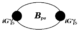
Figure 1: Meson dispersion loop graph $B_{ps}(P^{2})$.

$$B_{ps}(P^{2})=\int\limits^{\infty}_{(m_{1}+m_{2})^{2}}\frac{ds\;G^{2}(s)}{\pi(s-P^{2})}\rho_{ps}(s),\quad B_{ps}(M^{2})=1$$ (2)

with $\rho_{ps}(s)$ the spectral density of the Feynman loop graph

$$\rho_{ps}(s,m_{1},m_{2})=-\frac{1}{8\pi^{2}}\int dk_{1}dk_{2}\delta(k^{2}_{1}-m_{1}^{2})\delta(k^{2}_{2}-m_{2}^{2})\delta(P-k_{1}-k_{2})\;Sp\left({(\hat{k}_{1}+m_{1})i\gamma_{5}(m_{2}-\hat{k}_{2})i\gamma_{5}}\right)$$ (3)

$$=\frac{\lambda^{1/2}(s,m_{1}^{2},m_{2}^{2})}{8\pi s}(s-(m_{1}-m_{2})^{2})\;\theta(s-(m_{1}+m_{2})^{2}),$$

where

$$\lambda(s,m_{1}^{2},m_{2}^{2})\equiv(s+m^{2}_{1}-m^{2}_{2})^{2}-4sm_{1}^{2}.$$

Taking into account constituent–quark rescatterings leads to the renormalization of $G$ (see the Appendix A), and the soft constituent–quark structure of the pion is given by the vertex

$$\frac{\bar{Q}^{a}(k_{1},m_{1})i\gamma_{5}Q^{a}(-k_{2},m_{2})}{\sqrt{N_{c}}}G_{v}(P^{2})$$ (4)

where $G_{v}(s)=G(s)/B^{\prime}(M^{2})$,

$$\int\frac{G^{2}_{v}(s)\rho_{ps}(s,m_{1},m_{2})ds}{\pi(s-M^{2})^{2}}=1$$ (5)

Once the soft vertex (4) is fixed, we can proceed with calculating meson interaction amplitudes.

2.2 Weak decay of a pseudoscalar meson

Let us consider the decay $P\to\mu\nu$. The corresponding amplitude reads

$$<P|A^{aa}_{\mu}(0)|0>=iP_{\mu}\;f_{P},$$ (6)

$f_{P}$ is the meson axial–vector decay constant. To obtain the expression for this matrix element we must first consider the quantity

$$<Q\bar{Q}|A^{aa}_{\mu}(0)|0>$$ (7)

with $Q$ a constituent quark, while the axial current $A_{\mu}(0)=\bar{q}(0)\gamma_{\mu}\gamma_{5}q(0)$ is defined through current quarks. Next, we must single out the pole corresponding to the pion.

The $bare$ matrix element has the structure

$$<Q(k_{1})\bar{Q}(k_{2})|A^{aa}_{\mu}(0)|0>_{bare}=\bar{Q}(k_{1})\left[{\gamma_{\mu}\gamma_{5}g^{0}_{A}(P^{2})+P_{\mu}\gamma_{5}h^{0}_{+}(P^{2})+(k_{1}-k_{2})_{\mu}\gamma_{5}h^{0}_{-}(P^{2})}\right]Q(-k_{2})$$ (8)

If current quarks were identical to constituent ones we would have had

$$g_{A}^{0}(P^{2})\equiv 1,\quad h_{+}^{0}(P^{2})\equiv 0,\quad h_{-}^{0}(P^{2})\equiv 0.$$ (9)

It is reasonable to assume that at least at $P^{2}=(m_{1}-m_{2})^{2}$ the form factors $g$ and $h$ are not far from these values.

The rescatterings of the constituent quarks lead to the series of the dispersion graphs of Fig.2.

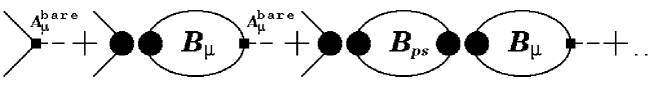
Figure 2: The series of dispersion graphs for $<Q\bar{Q}|A_{\mu}(0)|0>$.

The $bare$ matrix element enters into a single loop graph $B_{\mu}$ whose spectral density is the product of $G(s)$ and the corresponding Feynman graph spectral density which reads

$$-\frac{\sqrt{N_{c}}}{8\pi^{2}}\int dk_{1}dk_{2}\delta(k^{2}_{1}-m_{1}^{2})\delta(k^{2}_{2}-m_{2}^{2})\delta(P-k_{1}-k_{2})\;$$ (10)

$$\times Sp\left({[\gamma_{\mu}\gamma_{5}g_{A}^{0}(P^{2})+P_{\mu}\gamma_{5}h_{+}^{0}(P^{2})+(k_{1}-k_{2})_{\mu}\gamma_{5}h_{-}^{0}(P^{2})](\hat{k}_{1}+m_{1})\;i\gamma_{5}(m_{2}-\hat{k}_{2})}\right)$$

The trace is equal to

$$-4i(k_{1\mu}m_{2}+k_{2\mu}m_{1})g^{0}_{A}(P^{2})+4iP_{\mu}(k_{1}k_{2}+m_{1}m_{2})h^{0}_{+}(P^{2})+4i(k_{1}-k_{2})_{\mu}(k_{1}k_{2}+m_{1}m_{2})h^{0}_{-}(P^{2})$$ (11)

So the expression for the loop graph $B_{\mu}$ takes the form

$$B_{\mu}=4iP_{\mu}\sqrt{N_{c}}\int\limits_{(m_{1}+m_{2})^{2}}^{\infty}\frac{ds\;G(s)}{\pi(s-M^{2})}\frac{\lambda^{1/2}(s,m_{1}^{2},m_{2}^{2})}{16\pi s}\frac{s-(m_{1}-m_{2})^{2}}{2s}$$ (12)

$$\times[(m_{1}+m_{2})g_{A}^{0}(P^{2})-s\;h^{0}_{+}(P^{2})-(m_{1}^{2}-m_{2}^{2})h^{0}_{-}(P^{2})]$$

The amplitude with the quark rescatterings taken into account has the same spinorial structure as the $bare$ amplitude

$$<Q(k_{1})\bar{Q}(k_{2})|A^{aa}_{\mu}(0)|0>=\bar{Q}(k_{1})\left[{\gamma_{\mu}\gamma_{5}g_{A}(P^{2})+P_{\mu}\gamma_{5}h_{+}(P^{2})+(k_{1}-k_{2})_{\mu}\gamma_{5}h_{-}(P^{2})}\right]Q(-k_{2})$$ (13)

with

$$g_{A}(P^{2})=g_{A}^{0}(P^{2})$$

$$h_{-}(P^{2})=h_{-}^{0}(P^{2})$$

$$h_{+}(P^{2})=h_{+}^{0}(P^{2})-\frac{G(P^{2})}{1-B_{ps}(P^{2})}$$

$$\times\int\frac{ds\;G(s)}{\pi(s-M^{2})}\frac{\lambda^{1/2}(s,m_{1}^{2},m_{2}^{2})}{16\pi s}\frac{s-(m_{1}-m_{2})^{2}}{2s}4[(m_{1}+m_{2})g_{A}^{0}(P^{2})-s\;h^{0}_{+}(P^{2})-(m_{1}^{2}-m_{2}^{2})h^{0}_{-}(P^{2})]$$

The form factor $h_{+}$ develops a pole at $P^{2}=M^{2}$ as $B_{ps}(M^{2})=1$. Near $P^{2}=M^{2}$ the pole dominates the amplitude

$$<\bar{Q}Q|A_{\mu}|0>=<\bar{Q}Q|P>\frac{1}{M^{2}-P^{2}}<P|A_{\mu}|0>+{\rm regular\;terms}.$$ (14)

Comparing the pole terms in (13) and (14) and using the relation

$$<P|Q\bar{Q}>=\frac{\bar{Q}i\gamma_{5}Q}{\sqrt{N_{c}}}G_{v}$$

one finds

$$<P|A^{aa}_{\mu}(0)|0>=iP_{\mu}f_{P}$$ (15)

with

$$f_{P}=4\sqrt{N_{c}}\int\frac{ds\;G_{v}(s)}{\pi(s-M^{2})}\frac{\lambda^{1/2}(s,m_{1}^{2},m_{2}^{2})}{16\pi s}\frac{s-(m_{1}-m_{2})^{2}}{2s}$$ (16)

$$\times[(m_{1}+m_{2})g_{A}^{0}(P^{2})-s\;h^{0}_{+}(P^{2})-(m_{1}^{2}-m_{2}^{2})h^{0}_{-}(P^{2})]$$

Assuming that in reality the values of $g_{A}^{0}$ and $h^{0}$ are not far from the limit (9), we neglect the terms involving $h^{0}$ and come to the relation

$$f_{P}=4\sqrt{N_{c}}(m_{1}+m_{2})g_{A}^{0}(M^{2})\int\limits_{(m_{1}+m_{2})^{2}}^{\infty}\frac{ds\;G_{v}(s)}{\pi(s-M^{2})}\frac{\lambda^{1/2}(s,m_{1}^{2},m_{2}^{2})}{16\pi s}\frac{(s-(m_{1}-m_{2})^{2})}{2s}$$ (17)

2.3 The two-photon decay of the neutral pseudoscalar meson

We consider the decay of the neutral pseudoscalar meson $P_{0}$ whose constituent quark structure is described by the vertex

$$\frac{\bar{Q}i\gamma_{5}Q}{\sqrt{N_{c}}}G_{v}(P^{2})$$ (18)

The rate of the decay $P_{0}\to 2\gamma$ can be written as

$$\Gamma=\frac{\pi}{4}\alpha^{2}M^{3}g^{2}_{P\gamma\gamma},\quad g_{P\gamma\gamma}=G_{P\gamma\gamma}(M^{2},0,0),$$ (19)

where the form factor $G_{P\gamma\gamma}$ is connected with the amplitude

$$<0|J^{em}_{\alpha_{2}}(q_{2})J^{em}_{\alpha_{3}}(q_{3})|P>=2\epsilon_{\alpha_{2}\alpha_{3}\beta_{2}\beta_{3}}q_{2}^{\beta_{2}}q_{3}^{\beta_{3}}G_{P\gamma\gamma}(M^{2},q^{2}_{2},q^{2}_{3}).$$ (20)

The electromagnetic current $J^{em}_{\mu}(0)=\bar{q}(0)\gamma_{\mu}q(0)$ is defined through current quarks, whereas the meson structure is described in terms of the constituent quarks. So, for calculating the meson amplitude the constituent quark amplitude of the electromagnetic current is necessary. The latter is assumed to have the following structure

$$<Q(k^{\prime})|\bar{q}(0)\gamma_{\mu}q(0)|Q(k)>=\bar{Q}(k^{\prime})\gamma_{\mu}Q(k)f_{c}(q^{2}),\quad q=k^{\prime}-k.$$ (21)

The constituent charge form factor $f_{c}(q^{2})$ is normalized such that $f_{c}(0)=e_{c}$, the constituent charge. The anomalous magnetic moment of the constituent quark is neglected in the expression (21), but it can be included into consideration straightforwardly.

The single dispersion representation for the form factor $G_{P\gamma\gamma}$ reads

$$G_{P\gamma\gamma}(M^{2},s_{2},s_{3})=f_{c}(s_{2})f_{c}(s_{3})\int\frac{ds_{1}G_{v}(s_{1})}{\pi(s_{1}-M^{2})}\Delta_{P\gamma\gamma}(s_{1},s_{2},s_{3}),\quad s_{2}=q^{2}_{2},s_{3}=q^{2}_{3}$$ (22)

where $\Delta_{P\gamma\gamma}$ is determined by the spectral density of the Feynman graph of Fig.3

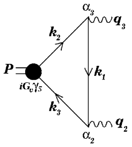
Figure 3: The graph describing the decay $P^{0}\to\gamma\gamma$.

$$-\frac{\sqrt{N_{c}}}{8\pi^{2}}\int dk_{1}dk_{2}dk_{3}\delta(P-k_{2}-k_{3})\delta(k_{2}-k_{1}-q_{3})\frac{\delta(k^{2}_{2}-m^{2})\delta(k^{3}_{2}-m^{2})}{m^{2}-k_{1}^{2}}$$

$$\times Sp\left({i\gamma_{5}(m-\hat{k}_{3})\gamma_{\alpha_{2}}(m+\hat{k}_{1})\gamma_{\alpha_{3}}(m+\hat{k}_{2})}\right)=-\epsilon_{\alpha_{2}\alpha_{3}\beta_{2}\beta_{3}}q_{2}^{\beta_{2}}q_{3}^{\beta_{3}}\Delta_{P\gamma\gamma}(s_{1},s_{2},s_{3})$$ (23)

The trace reads

$$Sp\left({i\gamma_{5}(m-\hat{k}_{3})\gamma_{\alpha_{2}}(m+\hat{k}_{1})\gamma_{\alpha_{3}}(m+\hat{k}_{2})}\right)=4m\epsilon_{\alpha_{2}\alpha_{3}\beta_{2}\beta_{3}}q_{2}^{\beta_{2}}q_{3}^{\beta_{3}},$$ (24)

and we find

$$\Delta_{P\gamma\gamma}(s_{1},s_{2},s_{3})=\frac{m\sqrt{N_{c}}}{4\pi}\frac{\theta(s_{1}-4m^{2})}{\lambda^{1/2}(s_{1},s_{2},s_{3})}\log\left({\frac{s_{1}-s_{2}-s_{3}+\lambda^{1/2}(s_{1},s_{2},s_{3})\sqrt{1-4m^{2}/s}}{s_{1}-s_{2}-s_{3}-\lambda^{1/2}(s_{1},s_{2},s_{3})\sqrt{1-4m^{2}/s}}}\right)$$ (25)

Substituting (25) into (22), one obtains the expression which defines the quantity $G_{P\gamma\gamma}$ for off-shell photons. For real photons one finds

$$g_{P\gamma\gamma}=\frac{m\sqrt{N_{c}}}{4\pi}e_{c}^{2}\int\limits_{4m^{2}}^{\infty}\frac{dsG_{v}(s)}{\pi(s-M^{2})}\frac{1}{s}\log\left({\frac{1+\sqrt{1-4m^{2}/s}}{1-\sqrt{1-4m^{2}/s}}}\right)$$ (26)

2.4 The elastic electromagnetic form factor

The elastic electromagnetic form factor of a pseudoscalar meson is given by the following matrix element

$$<P^{\prime}_{M}|J^{em}_{\mu}(0)|P_{M}>=(P^{\prime}_{M}+P_{M})_{\mu}\;F^{el}(q^{2})$$ (27)

$$P_{M}^{2}=P^{\prime 2}_{M}=M^{2},\;P_{M}-P^{\prime}_{M}=q,\;q^{2}<0.$$

Assuming the following structure for the constituent–quark matrix element of the electromagnetic current $J^{em}_{\mu}(0)=\bar{q}(0)\gamma_{\mu}q(0)$,

$$<Q(k^{\prime}_{1})|\bar{q}(0)\gamma_{\mu}q(0)|Q(k_{1})>=\bar{Q}(k^{\prime}_{1})\gamma_{\mu}Q(k_{1})\;f_{c}(q^{2}),$$ (28)

the elastic charge form factor of the meson can be written in the form

$$F^{el}(q^{2})=f_{1}(q^{2})H(q^{2},m_{1}^{2},m_{2}^{2})+f_{2}(q^{2})H(q^{2},m_{2}^{2},m_{1}^{2})$$ (29)

in terms of the form factors $H$. The quantity $H(q^{2},m_{1}^{2},m_{2}^{2})$ describes the subprocess when the constituent $1$ interacts with the photon, while the constituent $2$ remains spectator.

The double dispersion representation for the form factor $H(q^{2},m_{1}^{2},m_{2}^{2})$ (Fig.4) reads

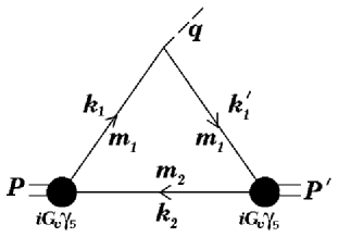
Figure 4: The contribution $H(q^{2},m_{1}^{2},m_{2}^{2})$ to the elastic form factor.

$$H(q^{2},m_{1}^{2},m_{2}^{2})=\int\frac{ds\;G_{v}(s)}{\pi(s-M^{2})}\frac{ds^{\prime}G_{v}(s^{\prime})}{\pi(s^{\prime}-M^{2})}\Delta(s^{\prime},s,q^{2}|m_{1},m_{1},m_{2}).$$ (30)

Here $\Delta$ is the double spectral density over $P^{2}$ and $P^{\prime 2}$ of the corresponding triangle Feynman graph

$$-\frac{1}{8\pi}\int dk_{1}dk^{\prime}_{1}dk_{2}\delta(k^{2}_{1}-m_{1}^{2})\delta(k^{\prime 2}_{1}-m_{1}^{2})\delta(k^{2}_{2}-m_{2}^{2})\delta(P-k_{1}-k_{2})\delta(P^{\prime}-k^{\prime}_{1}-k_{2})$$

$$\times Sp\left({(\hat{k}^{\prime}_{1}+m_{1})\gamma_{\mu}(\hat{k}_{1}+m_{1})i\gamma_{5}(m_{2}-\hat{k}_{2})i\gamma_{5}}\right)=2P_{\mu}(q)\Delta(s^{\prime},s,q^{2}|m_{1},m_{1},m_{2})$$ (31)

with

$$P_{\mu}(q)=(P-\frac{qP}{q^{2}}\,q)_{\mu},\;P^{2}=s,\;P^{\prime 2}=s^{\prime},\;(P^{\prime}-P)^{2}=q^{2}.$$

The trace reads

$$\frac{1}{4}Sp\left({(\hat{k}^{\prime}_{1}+m_{1})\gamma_{\mu}(\hat{k}_{1}+m_{1})\gamma_{5}(m_{2}-\hat{k}_{2})\gamma_{5}}\right)=2k^{\prime}_{1\mu}(s-(m_{1}-m_{2})^{2})+2k_{1\mu}(s^{\prime}-(m_{1}-m_{2})^{2})+2k_{2\mu}q^{2}$$ (32)

Multiplying both sides of (31) by $P_{\mu}$ and using (32) one obtains at $q^{2}<0$

$$\Delta(s^{\prime},s,q^{2}|m_{1},m_{1},m_{2})=\frac{-q^{2}}{4\lambda^{3/2}(s^{\prime},s,q^{2})}\left({s^{\prime}s+(s^{\prime}+s-q^{2})m_{2}(m_{1}-m_{2})-(m_{1}+m_{2})(m_{1}-m_{2})^{3}}\right)$$ (33)

$$\theta(s-(m_{1}+m_{2})^{2})\theta(s^{\prime}-(m_{1}+m_{2})^{2})\theta\left({-q^{2}(s^{\prime}+s-q^{2}+2(m_{1}^{2}-m_{2}^{2}))^{2}+\lambda(s^{\prime},s,q^{2})(q^{2}-4m_{1}^{2})}\right),\quad q^{2}<0$$

with $\lambda(s^{\prime},s,q^{2})=(s^{\prime}+s-q^{2})^{2}-4s^{\prime}s$.

At $q^{2}=0$ one finds

$$\Delta(s^{\prime},s,q^{2}=0|m_{1},m_{1},m_{2})=\pi\rho_{ps}(s,m_{1},m_{2})\;\delta(s^{\prime}-s),$$ (34)

and

$$F^{el}(0)=(e_{1}+e_{2})\int\limits_{(m_{1}+m_{2})^{2}}^{\infty}\frac{ds\;G_{v}^{2}(s)}{\pi(s-M^{2})^{2}}\rho_{ps}(s,m_{1},m_{2})=e_{1}+e_{2}$$ (35)

As we have pointed out in the Appendix A, this is just the Ward identity consequence.

To reveal the relationship between the dispersion integral (30) and the light–cone technique, we introduce the light–cone variables

$$k_{-}=\frac{1}{\sqrt{2}}(k_{0}-k_{z});\quad k_{+}=\frac{1}{\sqrt{2}}(k_{0}+k_{z});\quad k^{2}=2k_{+}k_{-}-k^{2}_{\perp};$$ (36)

into the integral representation for the form factor spectral density (31). We choose the reference frame in which

$$P_{\perp}=0,\quad q_{+}=0,\quad q^{2}_{\perp}=-q^{2}$$

that is possible at $q^{2}<0$. Performing $k_{-}$ integration and setting $(\mu=+)$ in both sides of (32) one finds

$$\Delta(s^{\prime},s,q^{2}|m_{1},m_{1},m_{2})=\frac{1}{16\pi}\int\frac{dxd^{2}k_{\perp}}{x(1-x)}\delta\left({s-\frac{m_{1}^{2}}{1-x}-\frac{m_{2}^{2}}{x}-\frac{k^{2}_{\perp}}{x(1-x)}}\right)$$ (37)

$$\times\delta\left({s^{\prime}-\frac{m_{1}^{2}}{1-x}-\frac{m_{2}^{2}}{x}-\frac{(k_{\perp}+xq_{\perp})^{2}}{x(1-x)}}\right)(s^{\prime}+s-2(m_{1}-m_{2})^{2}-\frac{x}{1-x}q^{2})$$

Here we denoted $x=k_{2+}/P_{+}$ and $k_{\perp}=k_{2\perp}$.

Substituting (37) into (30) and performing $s$ and $s^{\prime}$ integrations, one derives

$$H(q^{2}_{\perp},m_{1},m_{2})=\int dxd^{2}k_{\perp}\psi(x,k_{\perp})\psi(x,k_{\perp}+xq_{\perp})\beta(x,k_{\perp},q_{\perp})$$ (38)

where the radial light-cone wave function of a pseudoscalar meson is introduced

$$\psi(x,k_{\perp})=\frac{G_{v}(s)\sqrt{s-(m_{1}-m_{2})^{2}}}{\pi^{3/2}\sqrt{8}(s-M^{2})\sqrt{x(1-x)}},\qquad s=\frac{m_{1}^{2}}{1-x}+\frac{m_{2}^{2}}{x}+\frac{k^{2}_{\perp}}{x(1-x)}$$ (39)

$$\beta=\frac{s-(m_{1}-m_{2})^{2}+k_{\perp}q_{\perp}/(1-x)}{\sqrt{s-(m_{1}-m_{2})^{2}}\sqrt{s^{\prime}-(m_{1}-m_{2})^{2}}},\qquad\beta(q_{\perp}=0)=1$$

The quantity $\beta$ accounts for the contribution of spins. It is different from unity at $q_{\perp}\neq 0$ because both the spin-nonflip and spin-flip amplitudes of the interacting quark contribute. The eq.(35) is the normalization condition for the soft radial wave function

$$\int dx\;d^{2}k_{\perp}\;|\psi(x,k_{\perp})|^{2}=1.$$ (40)

In terms of this wave function, the pseudoscalar meson axial–vector decay constant $f_{P}$ is represented as

$$f_{P}=g_{A}\frac{\sqrt{N_{c}}}{\sqrt{2}\pi^{3/2}}\int{dx\;d^{2}k_{\perp}}\;\psi(x,k_{\perp})\frac{m_{2}(1-x)+m_{1}x}{\sqrt{s-(m_{1}-m_{2})^{2}}}$$ (41)

This expression can be easily deduced by introducing the light–cone variables into the dispersion representation (10), making use of (11) and examining the $\mu=+$ component of the axial current.

Similarly, introducing the light–cone variables into (23) yields the following expression for $g_{P\gamma\gamma}$

$$g_{P\gamma\gamma}=\frac{m\sqrt{N_{c}}}{\sqrt{2}\pi^{3/2}}\int\frac{dxd^{2}k_{\perp}}{\sqrt{x(1-x)}}\psi(x,k_{\perp})\frac{x}{(m^{2}+k^{2}_{\perp})\sqrt{s}}$$ (42)

The same expressions for the form factor, pseudoscalar meson electroweak constant, and the two–photon decay constant as (38)–(42) were derived within the light–cone approach in refs [7]–[9].

3 Form factors of meson transitions

In this section we examine the electroweak transitions of pseudoscalar mesons. First, we derive the dispersion representations for transition form factors at $q^{2}<0$ and demonstrate them to be equal to those obtained within the light–cone calculations. Second, these dispersion representations allow us to perform the analytic continuation and derive the form factors of semileptonic decays of pseudoscalar mesons at $q^{2}>0$ where the direct application of the light–cone technique is hampered by the contribution of pair–creation subprocesses.

3.1 The pseudoscalar meson transition form factor at $q^{2}<0$

The amplitude of the weak transition of pseudoscalar mesons $M_{1}\to M_{2}$ (Fig.5) is determined by the two form factors $F_{+}$ and $F_{-}$

$$<P_{M_{2}},M_{2}|V^{aa}_{\mu}|P_{M_{1}},M_{1}> = (P_{M_{1}}+P_{M_{2}})F_{+}(s_{3})+(P_{M_{1}}-P_{M_{2}})F_{-}(s_{3})$$ (43)

$$<P_{M_{2}},M_{2}|A^{aa}_{\mu}|P_{M_{1}},M_{1}> = 0,$$

$$P_{M_{2}}^{2}=M_{2}^{2},P_{M_{1}}^{2}=M_{1}^{2},P_{M_{1}}-P_{M_{2}}=P_{M_{3}},P_{M_{3}}^{2}=s_{3}$$

The weak currents are defined through current quarks

$$V^{aa}_{\mu}=\bar{q}_{1}(0)\gamma_{\mu}q_{2}(0),\quad A^{aa}_{\mu}=\bar{q}_{2}(0)\gamma_{\mu}\gamma_{5}q_{1}(0).$$ (44)

The structure of the mesons is described in terms of the constituent quarks by the vertices

$$M_{1}:\;\frac{\bar{Q}_{2}(k_{2})i\gamma_{5}Q_{3}(-k_{3})}{\sqrt{N_{c}}}G_{v1}(P_{1}^{2}),\quad M_{2}:\;\frac{\bar{Q}_{1}(k_{1})i\gamma_{5}Q_{3}(-k_{3})}{\sqrt{N_{c}}}G_{v2}(P_{2}^{2})$$ (45)

For calculating the tranition amplitude (43) we again need the constituent quark matrix element of the weak current which is taken in the form

$$<Q_{1}(k_{1})|\bar{q}_{1}(0)\gamma_{\mu}q_{2}(0)|Q_{2}(k_{2})>=\bar{Q}_{1}(k_{1})\gamma_{\mu}Q_{2}(k_{2})f_{21}(s_{3})$$ (46)

The dispersion representation for the form factors reads

$$F_{\pm}(s_{3})=f_{21}(s_{3})\int\frac{ds_{1}G_{v1}(s_{1})}{\pi(s_{1}-M_{1}^{2})}\frac{ds_{2}G_{v2}(s_{2})}{\pi(s_{2}-M_{2}^{2})}\Delta_{\pm}(s_{1},s_{2},s_{3}|m_{1},m_{2},m_{3})$$ (47)

Here $\Delta_{\pm}$ are the double spectral densities of the Feynman graph corresponding to Fig.5 in $s_{1}-$ and $s_{2}-$channels

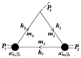
Figure 5: The dispersion graph for the decay $<P_{2}|V^{aa}_{\mu}|P_{!}>$.

$$-\frac{1}{8\pi}\int dk_{1}dk_{2}dk_{3}\delta(k^{2}_{1}-m_{1}^{2})\delta(k^{2}_{2}-m_{2}^{2})\delta(k^{3}_{2}-m_{3}^{2})\delta(P_{1}-k_{2}-k_{3})\delta(P_{2}-k_{3}-k_{1})$$

$$\times Sp\left({(\hat{k}_{1}+m_{1})\gamma_{\mu}(\hat{k}_{2}+m_{2})i\gamma_{5}(m_{3}-\hat{k}_{3})i\gamma_{5}}\right)=(P_{1}+P_{2})_{\mu}\Delta_{+}(s_{1},s_{2},s_{3}|m_{1},m_{2},m_{3})$$ (48)

$$+(P_{1}-P_{2})_{\mu}\Delta_{-}(s_{1},s_{2},s_{3}|m_{1},m_{2},m_{3})$$

with $P_{1}=P_{2}+P_{3}$, $P_{1}^{2}=s_{1}$, $P_{2}^{2}=s_{2}$, $P_{3}^{2}=P_{M_{3}}^{2}=s_{3}$. The vertices $G_{v1,2}$ are normalized in accordance with (5). The trace reads

$$Sp\left({(\hat{k}_{1}+m_{1})\gamma_{\mu}(\hat{k}_{2}+m_{2})\gamma_{5}(m_{3}-\hat{k}_{3})\gamma_{5}}\right)$$ (49)

$$=2k_{1\mu}(s_{1}-(m_{2}-m_{3})^{2})+2k_{2\mu}(s_{2}-(m_{3}-m_{1})^{2})+2k_{3\mu}(s_{3}-(m_{1}-m_{2})^{2})$$

$$=(P_{1}+P_{2}-2k_{3})_{\mu}\left({a(s_{1},m_{2},m_{3})+a(s_{2},m_{3},m_{1})-a(s_{3},m_{1},m_{2})}\right)$$

$$+(P_{1}+P_{2})_{\mu}a(s_{3},m_{1},m_{2})+(P_{1}-P_{2})_{\mu}\left({a(s_{2},m_{3},m_{1})-a(s_{1},m_{2},m_{3})}\right)$$

where $a(s,\mu_{1},\mu_{2})=s-(\mu_{1}-\mu_{2})^{2}$.

Making use of the relation

$$P_{1}+P_{2}-2k_{3}=\frac{b_{+}(s_{1},s_{2},s_{3})}{\lambda(s_{1},s_{2},s_{3})}(P_{1}+P_{2})+\frac{b_{-}(s_{1},s_{2},s_{3})}{\lambda(s_{1},s_{2},s_{3})}(P_{1}-P_{2})$$ (50)

with

$$b_{+}(s_{1},s_{2},s_{3}) = -s_{3}(s_{1}+s_{2}-s_{3}+m_{1}^{2}+m_{2}^{2}-2m_{3}^{2})-(m_{1}^{2}-m_{2}^{2})(s_{1}-s_{2})$$ (51)

$$b_{-}(s_{1},s_{2},s_{3}) = (m_{1}^{2}-m_{2}^{2})(2s_{1}+2s_{2}-s_{3})-(s_{1}-s_{2})(s_{1}+s_{2}-s_{3}+m_{1}^{2}+m_{2}^{2}-2m_{3}^{2}),$$ (52)

we come to the following result for $\Delta_{\pm}$

$$\Delta_{\pm}(s_{1},s_{2},s_{3}|m_{1},m_{2},m_{3})=\frac{B_{\pm}(s_{1},s_{2},s_{3})}{\lambda(s_{1},s_{2},s_{3})}\Delta(s_{1},s_{2},s_{3}|m_{1},m_{2},m_{3})$$ (53)

$$B_{+}(s_{1},s_{2},s_{3})=b_{+}(s_{1},s_{2},s_{3})(a(s_{1},m_{2},m_{3})+a(s_{2},m_{3},m_{1})-a(s_{3},m_{1},m_{2}))+a(s_{3},m_{1},m_{2})\lambda(s_{1},s_{2},s_{3})$$

$$B_{-}(s_{1},s_{2},s_{3})=b_{-}(s_{1},s_{2},s_{3})(a(s_{1},m_{2},m_{3})+a(s_{2},m_{3},m_{1})-a(s_{3},m_{1},m_{2}))$$

$$+(a(s_{2},m_{3},m_{1})-a(s_{1},m_{2},m_{3}))\lambda(s_{1},s_{2},s_{3})$$

Here $\Delta$, the double spectral density in $s_{1}$ and $s_{2}-$channels of the Feynman triangle graph $\Gamma(P_{1}^{2},P_{2}^{2},P_{3}^{2})$ with scalar constituents, is introduced

$$\Gamma(P_{1}^{2},P_{2}^{2},P_{3}^{2})=\frac{i}{(2\pi)^{4}}\int\frac{dk_{1}dk_{2}dk_{3}\delta(P_{1}-k_{2}-k_{3})\delta(P_{2}-k_{3}-k_{1})}{(m_{1}^{2}-k_{1}^{2}-i0)(m_{2}^{2}-k_{2}^{2}-i0)(m_{3}^{2}-k_{3}^{2}-i0)}$$ (54)

$$=\int\frac{ds_{1}}{\pi(s_{1}-M_{1}^{2})}\frac{ds_{2}}{\pi(s_{2}-M_{2}^{2})}\Delta(s_{1},s_{2},s_{3}|m_{1},m_{2},m_{3}).$$

At $s_{3}<0$ this spectral density reads

$$\Delta(s_{1},s_{2},s_{3}|m_{1},m_{2},m_{3})=\frac{\theta\left({-b_{+}^{2}(s_{1},s_{2},s_{3})-\lambda(s_{1},s_{2},s_{3})\lambda(s_{3},m_{1}^{2},m_{2}^{2})}\right)}{16\lambda^{1/2}(s_{1},s_{2},s_{3})},\quad s_{3}<0$$

The solution of this $\theta$-function reads

$$s_{2}>(m_{1}+m_{3})^{2},\quad s_{1}^{-}(s_{2},s_{3})<s_{1}<s_{1}^{+}(s_{2},s_{3});$$ (55)

$$s_{1}^{\pm}(s_{2},s_{3})=-\frac{1}{2m_{1}^{2}}$$

$$\times\left({s_{2}s_{3}-s_{2}(m_{1}^{2}+m_{2}^{2})-s_{3}(m_{1}^{2}+m_{3}^{2})+(m_{1}^{2}-m_{2}^{2})(m_{1}^{2}-m_{3}^{2})\pm\lambda^{1/2}(s_{2},m_{3}^{2},m_{1}^{2})\lambda^{1/2}(s_{3},m_{1}^{2},m_{2}^{2})}\right)$$

The final dispersion representation for the form factors at $s_{3}<0$ takes the form

$$F_{\pm}(s_{3})=f_{21}(s_{3})\int\limits^{\infty}_{(m_{1}+m_{3})^{2}}\frac{ds_{2}G_{v2}(s_{2})}{\pi(s_{2}-M_{2}^{2})}\int\limits^{s_{1}^{+}(s_{2},s_{3})}_{s_{1}^{-}(s_{2},s_{3})}\frac{ds_{1}G_{v1}(s_{1})}{\pi(s_{1}-M_{1}^{2})}\frac{B_{\pm}(s_{1},s_{2},s_{3})}{\lambda^{3/2}(s_{1},s_{2},s_{3})}$$ (56)

This representation will be the starting point for the consideration of the meson decays in the next section.

To demonstrate the equivalence of the dispersion method and the light–cone approach, we turn back to the equation (48) and again make use of the light–cone variables (36), choosing the reference frame $P_{M_{3}+}=0,P_{M_{1}\perp}=0$. Setting $\mu=+$ and making use of (49) gives for $\Delta_{+}$

$$\Delta_{+}(s_{1},s_{2},s_{3}|m_{1},m_{2},m_{3})=\frac{1}{16\pi}\int\frac{dx_{1}dx_{2}dx_{3}}{x_{1}x_{2}x_{3}}d^{2}k_{3\perp}\delta(x_{1}-x_{2})\delta(1-x_{1}-x_{3})$$ (57)

$$\times\delta\left({s_{1}-\frac{m_{2}^{2}}{x_{2}}-\frac{m_{3}^{2}}{x_{3}}-\frac{k^{2}_{3\perp}}{x_{2}x_{3}}}\right)\delta\left({s_{2}-\frac{m_{1}^{2}}{x_{1}}-\frac{m_{3}^{2}}{x_{3}}-\frac{(k_{3\perp}+x_{3}P_{3\perp})^{2}}{x_{2}x_{3}}}\right)$$

(Hereafter $x_{i}=k_{i+}/P_{+},P_{1+}=P_{2+}=P_{+},q_{\perp}=P_{3\perp},-q_{\perp}^{2}=s_{3},x\equiv x_{3},k_{\perp}\equiv k_{3\perp}$.) Substituting (57) into (47) yields the following expression for the form factor $F_{+}$ which gives the main contribution to the semileptonic meson decay rate

$$F_{+}(q_{\perp}^{2})=f_{21}(q_{\perp}^{2})\int\frac{dxd^{2}k_{\perp}}{16\pi^{3}x(1-x)}\frac{G_{v1}(s_{1})}{\pi(s_{1}-M_{1}^{2})}\frac{G_{v2}(s_{2})}{\pi(s_{2}-M_{2}^{2})}$$ (58)

$$\times\left({s_{1}+s_{2}-(m_{1}-m_{3})^{2}-(m_{2}-m_{3})^{2}+\frac{x}{1-x}(-q_{\perp}^{2}-(m_{1}-m_{2})^{2})}\right)$$

Introducing the radial light–cone wave funcion according to (39) leads to the familiar light–cone expression (cf.[7])

$$F_{+}(q_{\perp}^{2})=f_{21}(q_{\perp}^{2})\int dxd^{2}k_{\perp}\psi_{1}(x,k_{\perp})\psi_{2}(x,k_{\perp}+xq_{\perp})\beta_{+}(x,k_{\perp},q_{\perp});$$ (59)

$$\beta_{+}=\frac{s_{1}+s_{2}-(m_{1}-m_{3})^{2}-(m_{2}-m_{3})^{2}+\frac{x}{1-x}(-q_{\perp}^{2}-(m_{1}-m_{2})^{2})}{2\sqrt{s_{1}-(m_{2}-m_{3})^{2}}\sqrt{s_{2}-(m_{3}-m_{1})^{2}}}$$

$$=\frac{(m_{1}x+m_{3}(1-x))(m_{2}x+m_{3}(1-x))+k_{\perp}(k_{\perp}+xq_{\perp})}{x(1-x)\sqrt{s_{1}-(m_{2}-m_{3})^{2}}\sqrt{s_{2}-(m_{3}-m_{1})^{2}}}$$

3.2 The transition form factors at $q^{2}>0$

For the description of decay processes the form factors in the region $0<s_{3}<(M_{1}-M-2)^{2}$ are necessary, while the light–cone representation (59) is valid only at $s_{3}<0$. For deriving the form factors at $s_{3}>0$ the dispersion representation (56) turns out to be a convenient starting point. We write this representation in the following form

$$F(s_{3})=f_{21}(s_{3})\int\frac{ds_{1}G_{v1}(s_{1})}{\pi(s_{1}-M_{1}^{2})}\frac{ds_{2}G_{v2}(s_{2})}{\pi(s_{2}-M_{2}^{2})}\frac{B(s_{1},s_{2},s_{3})}{\lambda(s_{1},s_{2},s_{3})}\Delta(s_{1},s_{2},s_{3}|m_{1},m_{2},m_{3})$$ (60)

where $\Delta$ is the double spectral density of the Feynman graph $\Gamma$ with scalar constituents (54). This double dispersion representation defines the analytic function of $s_{3}$ both at negative and positive values provided the proper expression for the spectral density $\Delta$ is used. It is important to point out that the functions $G_{v}(s)$ have no singularities in the right–hand side of the complex $s$–plane [28], and $B$ and $\lambda$ are polynomials. So the details of the dispersion integration at $s_{3}>0$ are determined by the behavior of the quantity $\Delta$.

A detailed consideration of the double spectral density $\Delta$ for two massless constituents was performed in [10]. We extend that consideration to the case of arbitrary nonzero masses. The same analysis of $\Delta$ for arbitrary masses was done by Azimov [30].

Following [10], we first consider the single dispersion relation in $P_{2}^{2}$. A standard calculation yields

$$\Gamma(P_{1}^{2},P_{2}^{2},P_{3}^{2})=\int\limits_{(m_{1}+m_{3})^{2}}^{\infty}\frac{ds_{2}}{\pi(s_{2}-P_{2}^{2})}\sigma_{2}(P_{1}^{2},s_{2},P_{3}^{2}),$$ (61)

where

$$\sigma_{2}(P_{1}^{2},s_{2},P_{3}^{2})=\sigma_{+}(P_{1}^{2},s_{2},P_{3}^{2})-\sigma_{-}(P_{1}^{2},s_{2},P_{3}^{2}),$$ (62)

$$\sigma_{\pm}(s_{1},s_{2},s_{3})=\frac{1}{16\pi\lambda(s_{1},s_{2},s_{3})}\log\left({-s_{2}(s_{1}+s_{3}-s_{2}+m_{1}^{2}+m_{3}^{2}-2m_{2}^{2})-(s_{1}-s_{3})(m_{1}^{2}-m_{3}^{2})}\right).$$

Hereafter we assume $m_{2}>m_{1}$. The single dispersion representation reproduces the exact value of the Feynman expression (54). Next, we consider the function $\sigma_{2}(P_{1}^{2},s_{2},P_{3}^{2})$ as the analytic function of $s_{1}=P_{1}^{2}$ at fixed $s_{2}$ and $s_{3}=P_{3}^{2}>0$. As $s_{2}<s_{2}^{0}$ such that

$$\sqrt{s_{2}^{0}}=-\frac{s_{3}+m_{1}^{2}-m_{2}^{2}}{2\sqrt{s_{3}}}+\sqrt{\left({\frac{s_{3}+m_{1}^{2}-m_{2}^{2}}{2\sqrt{s_{3}}}}\right)^{2}+(m_{3}^{2}-m_{1}^{2})},\quad s_{3}<(m_{2}-m_{1})^{2},$$ (63)

both of the functions $\sigma_{+}$ and $\sigma_{-}$ have square–root branch points on the physical sheet at $s_{1}^{L}=(\sqrt{s_{2}}-\sqrt{s_{3}})^{2}$ and $s_{1}^{R}=(\sqrt{s_{2}}+\sqrt{s_{3}})^{2}$, connected by the cut (dashed line in Fig.6a).

Figure 6: The location of the singularities of $\sigma_{2}$ at $s_{3}>0$: a). $s_{2}<s_{2}^{0}$; b). $s_{2}>s_{2}^{0}$.

In addition, the function $\sigma_{-}$ has a logarithmic cut on the physical sheet from $s_{1}^{-}$ to $s_{1}^{+}$ defined by the expression (55). The square–root cuts cancel in $\sigma_{2}=\sigma_{+}-\sigma_{-}$, and the logarithmic cut is the only singularity of $\sigma_{2}$ on the physical sheet. The function $\sigma_{+}$ has also a logarithmic cut from $s_{1}^{-}$ to $s_{1}^{+}$ which is located on the second unphysical sheet of the Riemann surface of the square–root (dotted line in Fig.6a), and does not influence the double spectral density. The situation changes at $s_{2}=s_{2}^{0}$ which is determined by the condition $s_{1}^{R}(s_{2}^{0})=s_{1}^{-}(s_{2}^{0})$. The logarithmic and square–root branch points coincide, and for further increasing $s_{2}>s_{2}^{0}$ the logarithm branch point moves up through the square–root cut onto the physical sheet, whereas the position of the logarithm branch point of $\sigma_{-}$ goes to the second sheet (Fig.6b). Hence, on the physical sheet the function $\sigma_{+}$ acquires the logarithmic cut from $s_{1}^{-}$ to $s_{R}^{-}$, and $\sigma_{-}$ still has the logarithmic cut from $s_{1}^{-}$ to $s_{+}^{-}$. Both of the functions have also square–root branch cuts from $s_{1}^{L}$ to $s_{+}^{R}$. In the difference $\sigma_{2}=\sigma_{+}-\sigma_{-}$ the square–root cuts cancel each other, but the logarithmic cuts add. The resulting expression for the double spectral density takes the form

$$\Delta(s_{1},s_{2},s_{3}|m_{1},m_{2},m_{3})=\frac{\theta(s_{2}-(m_{1}+m_{3})^{2})\theta(s_{1}^{-}<s_{1}<s_{1}^{+})}{16\lambda^{1/2}(s_{1},s_{2},s_{3})}$$ (64)

$$+\frac{2\theta(s_{3})\theta(s_{2}-s_{2}^{0})\theta(s_{1}^{R}<s_{1}<s_{1}^{-})}{16\lambda^{1/2}(s_{1},s_{2},s_{3})}$$

One can check the double dispersion representation (54) with the spectral density $\Delta$ given by (64) to reproduce correctly the Feynman expression. The first term in (64) relates to the Landau–type contribution emerging when all intermediate particles go on mass shell, while the second term describes the non–Landau contribution.

In addition to the quantity $\Delta$, the spectral density of the representation (60) involves the factor $1/\lambda(s_{1},s_{2},s_{3})$ which is singular at the lower limit of the integration in the non–Landau term, namely

$$\lambda(s_{1},s_{2},s_{3})=(s-s_{1}^{L})(s-s_{1}^{R}).$$

As it has been discussed in [10], in this case an accurate application of the Cauchy theorem yields the subtracion term in the non–Landau contribution. Representing $\sigma_{2}$ as a contour integral, we must take into account the nonvanishing contribution of the small circle around the point $s_{1}^{R}$. Underline once more that the presence of the factor $G_{v1}(s_{1})$ does not change the argumentation as the function $G_{v}(s)$ has no singularities at $s_{1}>(m_{2}+m_{3})^{2}$. The final properly regularized representation for the form factors at $0<s_{3}<(m_{2}-m_{1})^{2}$ takes the form (omitting the constituent transition form factor $f_{21}(s_{3})$)

$$F(s_{3})=\int\limits_{(m_{1}+m_{3})^{2}}^{\infty}\frac{ds_{2}G_{v2}(s_{2})}{\pi(s_{2}-M_{2}^{2})}\int\limits_{s_{1}^{-}}^{s_{1}^{+}}\frac{ds_{1}G_{v1}(s_{1})}{\pi(s_{1}-M_{1}^{2})}\frac{B(s_{1},s_{2},s_{3})}{16\lambda(s_{1},s_{2},s_{3})}$$ (65)

$$+2\theta(s_{3})\int\limits_{s_{2}^{0}}^{\infty}\frac{ds_{2}G_{v2}(s_{2})}{\pi(s_{2}-M_{2}^{2})}\int\limits_{s_{1}^{R}}^{s_{1}^{-}}\frac{ds_{1}G_{v1}(s_{1})}{16\pi(s_{1}-s_{1}^{R})^{3/2}}\left[{\frac{G_{v1}(s_{1})B(s_{1},s_{2},s_{3})}{(s_{1}-s_{1}^{L})^{3/2}(s_{1}-M_{1}^{2})}-\frac{G_{v1}(s_{1}^{R})B(s_{1}^{R},s_{2},s_{3})}{(s_{1}^{R}-s_{1}^{L})^{3/2}(s_{1}^{R}-M_{1}^{2})}-}\right]$$

It should be pointed out, that although the representations (60) and (65) were deduced for the case of pseudoscalar mesons, transition form factors of any hadrons have the same structure. A particular choise of the initial and final hadrons yields a specific polynomial $B$. So the performed analysis is valid in the general case of hadron decay.

4 Calculation results

We are now in a position to apply the developed formalism to the analysis of the properties of pseudoscalar mesons and to the direct calculation of the decay form factors. To this end we must specify the parameters of the model, i.e. input the vertex functions of the pseudoscalar mesons and constituent quark masses.

4.1 Parameters of the model

For a pseudoscalar meson built up of quarks with the masses $m_{Q}$ and $m_{q}$, it is convenient to introduce the function $\phi$ related to the vertex function $G_{v}$ as

$$G_{v}(s)=\frac{\pi}{\sqrt{2}}\frac{\sqrt{s^{2}-(m_{Q}^{2}-m_{q}^{2})^{2}}}{\sqrt{s-(m_{Q}-m_{q})^{2}}}\frac{s-M^{2}}{s^{3/4}}\phi(k),\qquad k=\frac{\lambda^{1/2}(s,m_{Q}^{2},m_{q}^{2})}{2\sqrt{s}}$$ (66)

The normalization condition (5) for $G_{v}$ yields the following normalization condition for $\phi$

$$\int\phi^{2}(k)k^{2}dk=1.$$ (67)

The function $\phi$ is the ground–state $S$–wave radial wave function of a pseudoscalar meson for which we choose a simple exponential form

$$\phi(k)=\exp\left({-4\alpha\frac{k^{2}}{\mu^{2}_{P}}}\right)$$ (68)

where $\mu_{P}=m_{Q}m_{q}/(m_{Q}+m_{q})$ is the reduced mass. The parameterization (68) is inspired by the nonrelativistic quantum mechanics and, as we shall see later, is convenient for the analysis of the case $m_{Q}\to\infty$.

In the nonrelativistic quantum mechanics a bound–state wave function is determined by the motion of the particle with the mass $\mu_{P}$ in the potential independent of masses, and thus $\alpha$ does not depend on the masses as well. Relativistic effects destroy this simple feature of the wave function. In QCD the situation is much more complicated because additional dimensional quantities such as $\Lambda_{QCD}$ and the condensates appear. So, $\alpha$ should be considered as some unknown function of the quark masses. It is possible to obtain the information on the behavior of $\alpha$ as a function of $m_{Q}$ at fixed $m_{q}=m_{u,d}=0.25\;GeV$ in the two regions: at small $m_{Q}$ and $m_{Q}\to\infty$.

At $m_{Q}\leq 0.5\;GeV$ the value of $\alpha$ can be determined by describing the data in the light–meson sector. The light–quark masses given in Table 5 and $\alpha_{\pi}=\alpha_{K}=0.02$ provide a good description of the data on $f_{\pi}$, $f_{K}$, and the elastic form factors (Figs. 10 and 11). The meson decay constants and form factors are calculated with the values $g_{A}^{0}(M^{2})=1$ and $f_{c}(q^{2})=f_{c}(0)$, respectively.

In the region $m_{Q}\to\infty$ the behavior of $\alpha$ can be found on the basis of the heavy quark symmetry. To this end, let us consider the amplitudes of the elastic and inelstic transitions between pseudoscalar mesons consisting of heavy $Q$ and light $q$ quarks and introduce the dimensionless form factors as follows

$$<M,P^{\prime}|\bar{Q}\gamma_{\mu}Q|M,P>=(P^{\prime}+P)\;F_{el}(q^{2});\quad q^{2}\leq 0$$ (69)

$$F_{el}(q^{2})=h_{el}(\omega)=1-\rho^{2}_{el}(\omega-1)+O((\omega-1)^{2}),\quad\omega=1-\frac{q^{2}}{2M^{2}}\geq 1$$

$$<M_{2},P_{2}|\bar{Q}_{2}\gamma_{\mu}Q_{1}|M_{1},P_{1}>=(P_{1}+P_{2})F_{+}(q^{2})+(P_{1}-P_{2})F_{-}(q^{2});\qquad 0<q^{2}<(M_{1}-M_{2})^{2}$$ (70)

$$h_{\pm}(\omega)=\frac{M_{1}\pm M_{2}}{2\sqrt{M_{1}M_{2}}}F_{+}(q^{2})+\frac{M_{1}\mp M_{2}}{2\sqrt{M_{1}M_{2}}}F_{-}(q^{2});\quad\omega=\frac{M_{1}^{2}+M_{2}^{2}-q^{2}}{2M_{1}M_{2}}\geq 1.$$

$$h_{+}(\omega)=h_{+}(1)-\rho^{2}(\omega-1)+O((\omega-1)^{2}).$$

In the limit of infinitely heavy quarks $Q_{1,2}$, the amplitudes are expressed in terms of the single universal Isgur–Wise function (IW) $\xi(\omega$) [22]

$$h_{+}(\omega)=h_{el}(\omega)=\xi(\omega),\quad h_{-}(\omega)=0,\quad\xi(\omega)=1-\rho^{2}(\omega-1)+O((\omega-1)^{2}).$$ (71)

In addition, the qeavy quark symmetry predicts the universal relation for heavy–meson decay constants

$$\sqrt{M_{P}}f_{Q}=const.$$ (72)

The asymptotic relations (71) and (72) are the zero–order terms of the $1/m_{Q}$–expansion which is calculable within the HQET [21]. A particular form of the IW function depends on the heavy meson wave function.

The expressions (71) and (72) mean that the HQ symmetry restricts the possible behavior of the meson wave function at large $m_{Q}$. Table 4 gives the results on $f_{P}$ and $\rho^{2}_{el}$ vs $m_{Q}$ at $m_{q}=0.25\;GeV$, and Fig.9 presents the quantity $\sqrt{m_{Q}}f_{P}$ as the function of $m_{Q}$ for various values of $\alpha$. In the HQ limit, for a finite binding energy of the meson the heavy meson and the heavy quark masses coincide, $M_{Q}/m_{Q}=1$. So, the value of $\sqrt{m_{Q}}f_{P}$ should be independent of the heavy quark mass.

These results show that the asymptotic relations (71) and (72) are satisfied if the parameter $\alpha$ of the wave function (68) tends to a constant $\alpha_{\infty}$ as $m_{Q}\to\infty$.

Thus, the function $\alpha(m_{Q})$ has the following behavior: it is equal to 0.02 at $m_{Q}\leq 0.5\;GeV$ and tends to a constant $\alpha_{\infty}$ as $m_{Q}\to\infty$. For investigating the $B$ and $D$ mesons and their decays we need the information on $\alpha$ in the region $m_{Q}=2\div 5\;GeV$.

The simplest way is to extract $\alpha$ at $m_{Q}=2\div 5\;GeV$ from the analysis of $f_{D}$ and $f_{B}$ as we have done for the light mesons. In the absence of the experimental data we refer to the results of other models. As one can see, the decay constants $f_{P}$ calculated with $\alpha$ from the range $0.02\leq\alpha_{D},\alpha_{B}\leq 0.04$ cover the regions $160\;MeV\leq f_{D}\leq 230\;MeV$ and $130\;MeV\leq f_{B}\leq 200\;MeV$ which include the predictions of most of the models. Hence, the values of $\alpha_{D}$ and $\alpha_{B}$ related to the true wave functions of $D$ and $B$ mesons are expected to be inside the interval $0.02\div 0.04$.

However, there is an attractive possibility to specify $\alpha_{D,B}$ more precisely. Namely, it seems reasonable to assume $\alpha$ to be approximately constant in the region $m_{Q}\geq 1\div 2\;GeV$. There are at least two arguments behind this assumption. Firstly, a system consisting of a heavy and a light particles behaves like a quasinonrelativistic system. And secondly, there are no visible sources within QCD to yield steep changes of $\alpha$ in this region. Then for the $B$ and $D$ mesons one expects $\alpha_{D}=\alpha_{B}=\alpha_{\infty}$. The next step is to estimate $\alpha_{\infty}$. We consider the value $\alpha_{\infty}=0.02$ to be both attractive and reasonable: on the one hand, the same parameter describes all ground–state mesons, and on the other hand, one finds for $\alpha_{\infty}=0.02$

$$\sqrt{m_{\infty}}f_{P\infty}\simeq 5.8\;GeV^{3/2}$$

in agreement with the value $0.6\div 0.7$ estimated in [14].

Assuming $\alpha_{D}=\alpha_{B}=\alpha_{\infty}$, we can estimate the magnitude of the higher order $1/m_{Q}$ corrections which determine the deviations of the calculated $f_{P}$ and $\rho^{2}_{el}$ at finite $m_{Q}$ from the asymptotic relations (71) and (72). Rather strong violation of the HQ symmetry for $b-$ and $c-$quarks ($5\div 15$% at $m_{Q}=5\;GeV$ and $20\div 30$% at $m_{Q}=2\;GeV$) can be observed both in $f_{P}$ and $\rho^{2}_{el}$ at $\alpha_{\infty}=0.02\div 0.04$.

We shall analyze the transition form factors obtained at $\alpha_{D,B}=0.02$ and $0.04$. If our assumption $\alpha_{D}=\alpha_{B}=\alpha_{\infty}=0.02$ does not work properly, the form factor calculations for $\alpha=0.02$ and $\alpha=0.04$ give an interval which is expected to include the true value.

Table 5 gives the numerical parameters of the model.

4.2 Discussion

1. The results on the axial–vector decay constant $f_{P}$ are shown in Fig.9 and Table 4. Assuming $\alpha(m_{Q})=\alpha_{\infty}$ at $m_{Q}\geq 2\;GeV$, one can see the asymptotic relation $\sqrt{m_{Q}}f_{P}=const$ to work perfectly at $m_{Q}>40-50\;GeV$, and finds essential corrections to the asymptotic relations at lower $m_{Q}$. For $\alpha_{\infty}=0.02$ one obtains $f_{D}=234\;MeV$ and $f_{B}=202\;MeV$ that confirms the expectation $f_{D}\simeq f_{B}$ [13]. These values for the decay constants correspond to the constituent quark decay constant $g_{A}^{0}=1$. In reality, the latter can be less than unity, $g_{A}^{0}\simeq 0.75\div 1$. This will lead to decreasing the $f_{P}$.
2. Figures 12–17 present the elastic and transition form factors calculated with $\alpha_{D,B}=0.02$ and $0.04$.

The $K\to\pi$ transition form factor is well approximate by the linear function $F_{+}(q^{2})=F_{+}(0)+aq^{2}$, $F_{+}(0)=0.96$, $a=1.27\;GeV^{-2}$ in agreement with the results of [1].

The parameters of the monopole $F_{+}(q^{2})=F_{+}(0)/(1-q^{2}/M^{2}_{mon})$ and the dipole $F_{+}(q^{2})=F_{+}(0)/(1-q^{2}/M^{2}_{dip})^{2}$ fits to the other transition form factors are given in Table 6. The dipole formula excellently approximates the transition form factors with better than 1% accuracy. Although the monopole fit provides a worse accuracy, its parameters agree with the vector meson dominance. The values $F_{+}(0)$ are close to the corresponding results of QCD sum rules (cf. Tables 1 and 2) and the existing experimental data.
3. Fig.18 plots the IW function $\xi(\omega)=h_{+}(\omega)$ for the decay $B\to D$ at various values of $\alpha_{D}$ and $\alpha_{B}$. Table 8 gives the parameters of the calculated IW function. The function $h_{-}(\omega)$ turned out to be negligibly small in agreement with (71).

The IW function has been extensively studied both theoretically and experimentally (see Table 7). The analysis by ARGUS [31] and most of the earlier theoretical results suggested $1<\rho^{2}<2$. However, a recent analysis by CLEO as well as recent theoretical estimates favor the lower values $\rho^{2}\leq 1$. We found the relation $0.7\leq\rho^{2}\leq 0.9$ for all values of $\alpha_{D,B}$ from the considered interval.

As it follows from the HQ symmetry, the value $\xi(1)$ strongly depends on the relationship between $\alpha_{D}$ and $\alpha_{B}$: it turns out to be close to unity for $\alpha_{B}=\alpha_{D}$ and steeply decreases as $\alpha_{B}\neq\alpha_{D}$. One can find rather uncertain constraint for the considered region of the parameters $\alpha_{D,B}$ $0.87\leq\xi(1)\leq 0.98$.

Let us underline that except for the relationship between $\alpha_{D}$ and $\alpha_{B}$, the value $\xi(1)$ is also affected by the particular values of heavy–meson binding energies. At large quark masses and the binding energy kept finite, the heavy meson and heavy quark masses coincide, $M_{\infty}/m_{\infty}=1$. Hence, the positions of the ’quark zero recoil point’ $q_{0}^{2}=(m_{Q_{1}}-m_{Q_{2}})^{2}$ and the meson zero recoil point $q_{max}^{2}=(M_{1}-M_{2})^{2}$ also coincide. For infinitely heavy quarks this yields $\xi(1)=1$. For the physical heavy quarks and mesons, the positions of the ’quark zero recoil point’ $\omega_{0}=1-((m_{Q1}-m_{Q2})^{2}-(M_{1}-M_{2})^{2})/2M_{1}M_{2}$ and the ’meson zero recoil point’ $\omega=1$ do not coincide any longer. The calculated $\xi(\omega_{0})$ turns out to be not far from unity if $\alpha_{D}=\alpha_{B}$. So, the value $\xi(1)$ is sensitive to the particular values of the quark masses. The quark masses used in our calculation are chosen such that $m_{b}-m_{c}=M_{B}-M_{D}$, and thus $q^{2}_{0}=q^{2}_{max}$ and $\omega_{0}=1$. That is why $\xi(1)\simeq 1$ at $\alpha_{D}=\alpha_{B}$. For other reasonable values of quark masses, the deviation from unity at $\alpha_{D}=\alpha_{B}$ are found at the level of 3–4%.
4. The analysis of the analytic properties of the hadron transition form factors yields the following typical picture demonstrated in Fig.16: at $q^{2}\leq 0$ the contribution of the non–Landau singularity is absent, and the Landau–type singularity determines the form factor; in the region $0<q^{2}<(m_{2}-m_{1})^{2}$ both of them are essential; at the point $q^{2}=(m_{2}-m_{1})^{2}$ the contribution of the Landau singularity vanishes, and the non–Landau singularity determines the decay form factor at this ’quark zero recoil’ point.

For hadron decays related to the heavy–to–heavy quark transitions, a specific relationship between the Landau and the non–Landau contributions to the dispersion representation is observed: the normal Landau contribution dominates the form factor at all $q^{2}<(m_{2}-m_{1})^{2}$, whereas the anomalous singularity is essential only in the close vicinity of this point. So, effectively the transition form factor are determined by the contribution of the Landau contribution only. Thus, the HQ symmetry can be formulated in the language of the analytic properties of the transition form factors as the dominance of the Landau singularity in the almost whole kinematical region.

In the case of the meson decay related to a heavy–to–light quark transition, the anomalous non–Landau contribution is important in a broad kinematical region. So the relations suggested by the HQ symmetry would not work properly.

5 Conclusion

We investigated form factors of hadron transitions within the relativistic constituent quark model and proposed a formalism for a direct calculation of hadron decay form factors. The developed approach was applied to the analysis of the electroweak properties and transitions of pseudoscalar mesons. Our main results are:
1. The equivalence of the light–cone constituent quark model and the approach based on the dispersion relation integration over a bound state mass for the description of leptonic decays and transition form factors at spacelike momentum transfers has been demonstrated. Although the comparison has been performed for a particular case of pseudoscalar mesons, the approaches are equivalent for the description of any hadrons.
2. The obtained dispersion formulation of the light–cone constituent quark model allows a consideration of the decay processes where the direct application of the light–cone technique is hampered by the contribution of pair–creation subprocesses. The analytic continuation in the dispersion representation of the transition form factor yields the form factor at timelike momentum transfers expressed through the meson radial light–cone wave function. Along with the normal Landau singularities, the anomalous non–Landau singularities contribute to the form factors at $q^{2}>0$.
3. For hadron decays related to the heavy–to–heavy quark transitions a specific relationship between the contributions of the Landau–type and the non–Landau singularities has been observed. This allows a formulation of the heavy quark symmetry in the language of the analytic properties of the decay form factors as the dominance of the normal Landau contribution in the almost whole kinematic region of momentum transfers.
4. Electroweak properties and form factors of pseudoscalar mesons have been analyzed using a parameterization of the meson wave function based on the heavy quark symmetry. We have examined the dependence of the axial–vector decay constant on the heavy–quark mass, and found $f_{D}\simeq 235\;MeV$ and $f_{B}\simeq 200\;MeV$. These values can be decreased by a factor of $0.75\div 1$, if the decay constant at the level of the constituen quarks is less than unity.

The correlation between the axial–vector decay constant $f_{P}$ and the transition form factors yields the IW function parameter $\rho^{2}=0.8\pm 0.1$ for the axial–vector decay constants from the intervals $160\;MeV\leq f_{D}\leq 235\;MeV$ and $130\;MeV\leq f_{D}\leq 200\;MeV$

Analyzing the dependence of $f_{P}$ and the heavy meson form factor on the heavy quark mass we have found that the violation of the HQ symmetry relations can be expected at the 10–20% level for the $b$– and $c$–quark masses .
5. The calculated form factors of pseudoscalar meson transitions have been approximated with a 1%–accuracy by the dipole formula in the whole kinematic region. The form factors are also compatible with the vector meson dominance and are close to the results of the QCD sum rules.

The developed approach can be applied to the description of the pseudoscalar–to–vector meson transitions and rare decays of heavy mesons. This work is now in progress.

I am grateful to V.V.Anisovich, Ya.I.Azimov, and K.A.Ter–Martirosyan for discussing the general problems and technical details related to hadron decays. I am also indebted to the German Ministry of Science and Technology for the financial support at the early stage of this work and to H.R.Petry for his hospitality during my stay in Bonn.

Table 1: The form factors of the decays $B\to\pi,\rho$ at $q^{2}=0$. The labels Lat, SR, QM and LCQM stand for Lattice, Sum Rules, Quark Model and Light Cone Quark Model, respectively.

		$F_{+}(0)$	$V(0)$	$A_{1}(0)$	$A_{2}(0)$	$V(0)/A_{1}(0)$	$A_{2}(0)/A_{1}(0)$
Lat	[16]a	0.29$\pm$ 0.06	0.45$\pm$0.22	0.29$\pm$0.16	0.24$\pm$ 0.56	2.0$\pm$0.9	0.8$\pm$1.5
	[16]b	0.35$\pm$ 0.08	0.53$\pm$0.31	0.24$\pm$0.12	0.27$\pm$ 0.80	2.6$\pm$1.9	1.0$\pm$3.1
	[17]a	0.26$\pm$ 0.16	0.34$\pm$0.10	0.25$\pm$0.06	0.38$\pm$ 0.22	1.4$\pm$0.2	1.5$\pm$0.7
	[17]b	0.30$\pm$ 0.19	0.37$\pm$0.11	0.22$\pm$0.05	0.49$\pm$ 0.26	1.6$\pm$0.3	2.3$\pm$0.9
SR	[10]	0.24$\pm$ 0.025	–	–	–	–	–
	[12]	0.40$\pm$ 0.20	–	–	–	–	–
QM	WSB[2]	0.33	0.33	0.28	0.28	1.2	1.0
	GISW[4]	0.09	0.27	0.05	0.02	5.4	0.4

Table 2: The form factors of the decays $D\to K,K^{*}$ at $q^{2}=0$.

		$F_{+}(0)$	$V(0)$	$A_{1}(0)$	$A_{2}(0)$	$V(0)/A_{1}(0)$	$A_{2}(0)/A_{1}(0)$
Exp	[24]	0.77$\pm$ 0.04	1.16$\pm$0.16	0.61$\pm$0.05	0.45$\pm$ 0.09	1.90$\pm$0.25	0.74$\pm$0.15
Lat	[16]	0.78$\pm$ 0.08	1.08$\pm$0.22	0.67$\pm$0.11	0.49$\pm$ 0.34	1.6$\pm$0.3	0.7$\pm$0.4
	[17]	0.60$\pm$ 0.22	0.86$\pm$0.24	0.64$\pm$0.16	0.40$\pm$ 0.32	1.3$\pm$0.2	0.6$\pm$0.3
SR	[11]	0.6$\pm$ 0.15	1.1$\pm$ 0.25	0.5$\pm$ 0.15	0.6$\pm$ 0.1	2.2$\pm$0.2	1.2$\pm$ 0.2
QM	WSB[2]	0.76	1.23	0.88	1.15	1.4	1.3
	GISW[4]	0.8	1.10	0.80	0.80	1.4	1.0
LCQM	[7]	0.73	0.92	0.63	0.42	1.46	0.67

Table 3: The decay constants $f_{P}$ of pseudoscalar mesons $MeV$.

	$\pi$	$K$	$D$	$B$
Exp [25]	130.7$\pm$ 0.46	159.8$\pm$1.9	$<$ 310	–
Lattice [19]			200$\pm$ 30	180$\pm$ 40
Sum Rules	–	–	160 [11]	–
	–	–	165$\div$195[14]	130$\div$ 200[14]
LCQM [9]	130.7	162	220	188
LCQM[8]	130.7	162	206	186
This work	130	160	234	202

Table 4: The decay constants $f_{P}$ of pseudoscalar mesons built up of quarks with the masses $m_{Q}$ and $m_{q}$ and the slope of $h_{el}$ at $\omega=1$ calculated from $<M_{Q}|\bar{Q}\gamma_{\mu}Q|M_{Q}>$ as functions of $m_{Q}$ at $m_{q}=0.25\;GeV$.

	$\alpha=0.01$		$\alpha=0.02$		$\alpha=0.04$		$\alpha=0.08$
$m_{Q},GeV$	$f_{P},MeV$	$\rho^{2}_{el}$	$f_{P},MeV$	$\rho^{2}_{el}$	$f_{P},MeV$	$\rho^{2}_{el}$	$f_{P},MeV$	$\rho^{2}_{el}$
0.25	151	0.04	130	0.06	104	0.08	80	0.1
0.4	190	0.25	160	0.35	128	0.5	97	0.65
1.8	324	0.6	234	0.65	163	0.82	110	1.0
5.2	308	0.75	202	1.0	132	1.05	85	1.1
10	254	1.0	162	1.05	102	1.1	64	1.25
20	195	1.0	122	1.1	76	1.23	48	1.45
40	143	1.0	89	1.11	55	1.25	34	1.66
80	103	1.0	63	1.11	39	1.25	24	1.66

Table 5: The constituent quark masses and the calculated $f_{P}$ for $\alpha=0.02$.

quark	quark mass,$GeV$	meson	meson mass,$GeV$	$f_{P},MeV$
u,d	0.25	$\pi^{+}(u\bar{d})$	0.14	130
s	0.40	$K^{+}(u\bar{s})$	0.49	160
c	1.80	$D^{+}(c\bar{d})$	1.87	234
b	5.20	$B^{+}(u\bar{b})$	5.27	202

Table 6: The parameters of the monopole and dipole fits to the $F_{+}$ form factor. The masses of the lowest vector mesons which are expected to dominate the form factors are given in brackets.

	$\alpha_{B}=\alpha_{D}=0.02$			$\alpha_{B}=\alpha_{D}=0.04$
Decay	$F_{+}(0)$	$M_{mon},\;GeV$	$M_{dip},\;GeV$	$F_{+}(0)$	$M_{dip},\;GeV$
$B\to D$	0.73	5.7	7.7	0.68	7.20
$B\to\pi$	0.23	5.2 [5.324]	6.2	0.22	6.08
$D\to K$	0.70	2.22 [2.11]	3.0	0.70	2.95
$D\to\pi$	0.55	2.1 [2.01]	2.8	0.59	2.68

Table 7: The slope of the IW function $\rho^{2}$

	ARGUS [31]	CLEO [32]	Lat [18]	SR[15]	SR[33]	This work
$\rho^{2}$	$1.07\pm 0.17$	$0.87\pm 0.12$	1.2	$>1.04$	$0.7\pm 0.2$	$0.8\pm 0.1$

Table 8: The parameters of the IW function.

$\alpha_{D}$	$\alpha_{B}$	$\xi(1)$	$\rho^{2}$
0.02	0.02	0.98	0.78
0.02	0.04	0.87	0.75
0.04	0.02	0.93	0.7
0.04	0.04	0.98	0.88

6 Appendix A: Bound state description within dispersion relations

To illustrate main points of the dispersion approach we consider the case of two spinless constituents with the masses $m_{1}$ and $m_{2}$ interacting via exchanges of a meson with the mass $\mu$. We start with the scattering amplitude

$$A(s,t)=<k^{\prime}_{1},k^{\prime}_{2}|S|k_{1},k_{2}>,\quad s=(k_{1}+k_{2})^{2},\;t=(k_{1}-k^{\prime}_{1})^{2}$$ (73)

The amplitude as a function of $s$ has the threshold singularities in the complex $s$-plane connected with elastic rescatterings of the constituents and production of new mesons at

$$s=(m_{1}+m_{2})^{2},\;(m_{1}+m_{2}+\mu)^{2},\;(m_{1}+m_{2}+2\mu)^{2}\ldots$$ (74)

We assume that an $S$-wave bound state with the mass $M<m_{1}+m_{2}$ exists, then the partial amplitude $A_{0}(s)$ has a pole at $s=M^{2}$. The amplitude $A(s,t)$ has also $t$-channel singularities at $t=(n\mu)^{2};\;\;n=1,2,3\ldots$ connected with meson exchanges. If one needs to construct the amplitude in the low-energy region $s\geq(m_{1}+m_{2})^{2}$ the dispersion $N/D$ representation turns out to be convenient. Consider the $S$-wave partial amplitude

$$A_{0}(s)=\int\limits^{1}_{-1}dz\,A(s,t(s,z)),$$ (75)

where $t(z)=-(1-z)\lambda(s,m_{1}^{2},m_{2}^{2})/2s$, $z=\cos\theta$ in the c.m.s. The $A_{0}(s)$ as a function of complex $s$ has the right-hand singularities related to $s$-channel singularities of $A(s,t)$. In addition, it has left-hand singularities located at $s=(m_{1}+m_{2})^{2}-(n\mu)^{2};\;\;n=1,2,3\ldots$. They come from $t$-channel singularities of $A(s,t)$. The unitarity condition in the region $s\approx(m_{1}+m_{2})^{2}$ reads

$${\rm Im}\,A_{0}(s)=\rho(s)\;|A_{0}(s)|^{2},\qquad\rho(s)=\frac{\lambda(s,m_{1}^{2},m_{2}^{2})}{16\pi s}$$ (76)

with $\rho(s)$ the two-particle phase space. The $N/D$ method represents the partial amplitude as $A_{0}(s)=N(s)/D(s)$, where the function $N$ has only left-hand singularities and $D$ has only right-hand ones. The unitarity condition yields

$$D(s)=1-\int\limits^{\infty}_{(m_{1}+m_{2})^{2}}\frac{d\tilde{s}}{\pi}\,\frac{\rho(\tilde{s})N(\tilde{s})}{\tilde{s}-s}\;\equiv\;1-B(s).$$ (77)

Assuming the function $N$ to be positive we introduce $G(s)=\sqrt{N(s)}$. Then the partial amplitude takes the form

$$A_{0}(s)=G(s)\left[1+B(s)+B^{2}(s)+B^{3}(s)+\ldots\right]G(s)=\frac{G(s)G(s)}{1-B(s)}.$$ (78)

This expression can be interpreted as a series of loop diagrams of Fig.7

Figure 7: One of the terms in the expansion of $A_{0}(s)$

with the basic loop diagram

$$B(s)=\int\limits^{\infty}_{(m_{1}+m_{2})^{2}}\frac{d\tilde{s}}{\pi}\,\frac{\rho(\tilde{s})\;G^{2}(\tilde{s})}{\tilde{s}-s}.$$ (79)

The bound state with the mass $M$ relates to a pole both in the total and partial amplitudes at $s=M^{2}$ so $B(M^{2})=1$. Near the pole one has for the total amplitude

$$A = <k^{\prime}_{1},k^{\prime}_{2}|P>\frac{1}{M^{2}-P^{2}}<P|k_{1},k_{2}>+{\rm regular\;terms}$$ (80)

$$\equiv \chi^{*}_{P}(k^{\prime}_{1},k^{\prime}_{2})\frac{1}{M^{2}-P^{2}}\chi_{P}(k_{1},k_{2})+\ldots$$

where $\chi_{P}(k_{1},k_{2})$ is the amputated Bethe-Salpeter amplitude of the bound state. The dispersion amplitude near the pole reads

$$A=N/D+{\rm regular\;terms\;related\;to\;other\;partial\;waves}$$

$$=\frac{G^{2}(M^{2})}{(M^{2}-s)B^{\prime}(M^{2})}+\ldots\equiv\frac{G_{v}^{2}(M^{2})}{M^{2}-s}+\ldots$$ (81)

where $G_{v}$ is a vertex of the bound state transition to the constituents. The singular terms correspond to each other and hence

$$\chi_{P}(k_{1},k_{2})\to G_{v}(P^{2})\equiv\frac{G(P^{2})}{\sqrt{B^{\prime}(M^{2})}}$$ (82)

Underline that among right-hand singularities the constructed dispersion amplitude takes into account only the two-particle cut.

Let us turn to the interaction of the two-constituent system with an external electromagnetic field. The amplitude of this process $T_{\mu}=<k^{\prime}_{1},k^{\prime}_{2}|J_{\mu}(q)|k_{1},k_{2}>$ in the case of a bound state takes the form

$$T_{\mu} = <k^{\prime}_{1},k^{\prime}_{2}|P^{\prime}>\frac{1}{P^{\prime 2}-M^{2}}<P^{\prime}|J_{\mu}(q)|P>\frac{1}{P^{2}-M^{2}}<P|k_{1},k_{2}>+\ldots$$ (83)

$$= \chi^{*}_{P}(k^{\prime}_{1},k^{\prime}_{2})\frac{1}{P^{\prime 2}-M^{2}}(P^{\prime}+P)_{\mu}F(q^{2})\frac{1}{P^{2}-M^{2}}\chi_{P}(k_{1},k_{2})+\ldots$$

where the bound state form factor is defined as

$$<P^{\prime}|J_{\mu}(q)|P>=(P^{\prime}+P)_{\mu}F(q^{2})$$ (84)

The dispersion amplitude $T_{\mu}$ with only two-particle singularities in the $P^{2}$- and $P^{\prime 2}$-channels taken into account is given [28] by the series of graphs in Fig.8.

Figure 8: One of the terms in the series for $T_{\mu}$.

These graphs are obtained from the dispersion scattering amplitude series by inserting a photon line into constituent lines. The amplitude reads

$$T_{\mu}(P^{\prime},P,q)=2P_{\mu}(q)T(s^{\prime},s,q^{2})+\frac{q_{\mu}}{q^{2}}C,$$ (85)

$$P^{2}=s,\;P^{\prime 2}=s^{\prime},\;q=P^{\prime}-P,\;P_{\mu}(q)=(P-\frac{qP}{q^{2}}\,q)_{\mu}$$

The dispersion method allows one to determine $T(s,s^{\prime},q^{2})$, which is the part of the amplitude transverse with respect to $q_{\mu}$. Summing up the series of dispersion graphs in Fig.2 gives

$$T(s^{\prime},s,q^{2})=\frac{G(s)}{1-B(s)}\Gamma(s^{\prime},s,q^{2})\frac{G(s^{\prime})}{1-B(s^{\prime})}.$$ (86)

Here

$$\Gamma(s^{\prime},s,q^{2})=\int\frac{d\tilde{s}G(\tilde{s})}{\pi(\tilde{s}-s)}\frac{d\tilde{s}^{\prime}G(\tilde{s}^{\prime})}{\pi(\tilde{s}^{\prime}-s)}\Delta(\tilde{s}^{\prime},\tilde{s},q^{2}),$$

and $\Delta(\tilde{s}^{\prime},\tilde{s},q^{2})$ is the double spectral density of the three-point Feynman graph with a pointlike vertex of the constituent interaction.

The longitudinal part $C$ is given by the Ward identity

$$C=\frac{G(s)}{1-B(s)}\left({B(s^{\prime})-B(s)}\right)\frac{G(s^{\prime})}{1-B(s^{\prime})}$$ (87)

At $s=s^{\prime}=M^{2}$, the quantity $T_{\mu}$ develops both $s$ and $s^{\prime}$ poles, so

$$T_{\mu}(P^{\prime},P,q)=\frac{G_{v}(M^{2})}{M^{2}-s}(P^{\prime}+P)_{\mu}F(q^{2})\frac{G_{v}(M^{2})}{M^{2}-s^{\prime}}+{\rm less\;singular\;terms}$$ (88)

where

$$F(q^{2})=\int\limits_{(m_{1}+m_{2})^{2}}^{\infty}\frac{dsG_{v}(s)}{\pi(s-M^{2})}\frac{ds^{\prime}G_{v}(s^{\prime})}{\pi(s^{\prime}-M^{2})}\Delta(s^{\prime},s,q^{2}).$$ (89)

is the bound–state form factor (see (82) and (83)). So, the quantity $<P^{\prime}|J_{\mu}(q)|P>$ corresponds to the three–point dispersion graph with the vertices $G_{v}$. The following relation is valid $\Delta(s^{\prime},s,0)=\pi\delta(s^{\prime}-s)\rho(s)$. This is a consequence of the Ward identity which relates the three-point graph at zero momentum transfer to the loop graph. This relation yields the charge normalization $F(0)=1$. The expression (89) gives the form factor in terms of the $N$-function of the constituent scattering amplitude and double spectral density of the Feynman graph. In general, the following prescription works: to obtain the dispersion expression spectral density in channels corresponding to a bound state, one should calculate the related Feynman graph spectral density and multiply it by $G_{v}$.

If the constituent is a nonpoint particle, the expression (89) should be multiplied by form factor of an on-shell constituent.

Figure 9: The quantity $m_{Q}^{0.5}f_{P}$ as the function of $m_{Q}$ at $m_{q}=0.25\;GeV$.

Figure 10: The $\pi^{+}$ form factor, $\alpha_{\pi}=0.02$.

Figure 11: The $K^{+}$ form factor, $\alpha_{K}=0.02$.

Figure 12: The $D^{+}$ form factor. Solid – $\alpha_{D}=0.02$, dotted – $\alpha_{D}=0.04$.

Figure 13: The $B^{+}$ form factor. Solid – $\alpha_{B}=0.02$, dotted – $\alpha_{B}=0.04$.

Figure 14: The form factor $F_{+}(q^{2})$ for $B\to D$. Solid – $\alpha_{D}=\alpha_{B}=0.02$, dotted - the monopole fit, dash–dotted – the dipole fit. Dashed – $\alpha_{D}=\alpha_{B}=0.04$

Figure 15: The form factor $F_{+}(q^{2})$ for $B\to\pi$. Solid – $\alpha_{B}=0.02$, dotted - the monopole fit, dash–dotted – the dipole fit. Dashed – $\alpha_{B}=0.04$.

Figure 16: The form factor $F_{+}$ for $D\to K$. Solid – $\alpha_{D}=0.02$, dotted - the monopole fit, dash–dotted – the dipole fit. Long–dashed – the Landau singularity contribution, long–dash–dotted – the non-Landau term. Dashed – $\alpha_{D}=0.04$.

Figure 17: The form factor $F_{+}$ for $D\to\pi$. Solid – $\alpha_{D}=0.02$, dotted - the monopole fit, dash–dotted – the dipole fit. Dashed – $\alpha_{D}=0.04$.

Figure 18: The Isgur–Wise function $\xi(\omega)=h_{+}(\omega)$ of the decay $B\to D$: Solid – $\alpha_{D}=\alpha_{B}=0.02$, dashed – $\alpha_{D}=\alpha_{B}=0.04$, dash-dotted – $\alpha_{D}=0.04,\;\alpha_{B}=0.02$, dotted – $\alpha_{D}=0.02,\;\alpha_{B}=0.04$.

References

- [1] H.Leutwyler and M.Roos, Z.Phys. C25,91 (1984).
-
[2]
M.Wirbel, B.Stech, and M.Bauer, Z.Phys. C29, 637 (1985);
M.Bauer and M.Wirbel, Z.Phys. C42, 671 (1989). - [3] S.Godfrey and N.Isgur, Phys.Rev. D32, 189 (1985).
- [4] B.Grinstein, N.Isgur, D.Scora, and M.Wise, Phys.Rev. D39,799 (1989).
- [5] T.Altomary and L.Wolfenstein, Phys.Rev. D37, 681 (1988).
- [6] D.Scora and N.Isgur, Phys.Rev. D40, 1491 (1989).
- [7] W.Jaus, Phys.Rev. D44, 2319 (1991).
- [8] F.Schlumpf, SLAC-PUB-6483, hep-ph 9406267 (1994).
- [9] F.Cardarelli et al., Preprint INFN–ISS 94/3 (1994).
- [10] P.Ball, V.Braun, and H.Dosch, Phys.Lett. B273, 316 (1991).
- [11] P.Ball, V.Braun, and H.Dosch, Phys.Rev. D44, 3567 (1991).
- [12] P.Ball, Phys.Rev. D48, 3190 (1993).
- [13] S.Narison and K.Zalewski, Phys.Lett. B320, 369 (1994).
- [14] S.Narison, Phys.Lett. B322, 247 (1994).
- [15] S.Narison, Phys.Lett. B325, 197 (1994).
- [16] A.Abada et al., Nucl.Phys. B416, 675 (1994).
- [17] C.Allton et al., CERN-TH.7484/94 (1994).
- [18] S.Booth et al., Phys.Rev.Lett. 72, 462 (1994).
- [19] C.Sachrajda, Talk given at the EPC Conference (July, 1993, Marseille).
- [20] A.Le Yaouanc, Nucl.Instr.Meth. A351, 15 (1994).
-
[21]
D.Politzer and M.Wise, Phys.Lett. B208, 504 (1988);
H.Georgi, Phys.Lett. B240, 447 (1990). - [22] N.Isgur and M.Wise, Phys.Lett. B232, 113 (1989); Phys.Lett. B237, 527 (1990).
- [23] M.Neubert, Preprint SLAC-PUB-6263 (1993).
- [24] M.Witherell, XVI International Symposium on Lepton–Photon Interactions, Cornell University, Ithaca, NY, USA, 10–15 August 1993, UCSB-HEP-93-06 (1993).
- [25] Particle Data Group, Phys.Rev D50, 1443 (1994).
-
[26]
M.V.Terent’ev, Sov.J.Nucl.Phys. 24, 106 (1976);
V.B.Berestetskii and M.V.Terent’ev, Sov. J. Nucl. Phys. 24, 547 (1976); 25, 347 (1977). - [27] P.Chung, F.Coester, and W.Polyzou, Phys.Lett. B205, 545 (1988).
- [28] V.V.Anisovich, M.N.Kobrinsky, D.I.Melikhov, and A.V.Sarantsev, Nucl.Phys. A544, 747 (1992).
- [29] V.V.Anisovich, D.I.Melikhov, B.C.Metsch, and H.R.Petry, Nucl.Phys. A563, 549 (1993).
- [30] Ya.Azimov, private communication.
- [31] ARGUS Collabortion: H.Albrecht et al., Phys.Lett. B275, 195 (1992), Z.Phys. C75, 533 (1993).
- [32] CLEO Collaboration: B.Barish et al., Preprint CLNS 94/125 (1994).
- [33] M.Neubert, Phys.Lett. B338, 84 (1994).