Abstract

The purely nonperturbative soft contribution to the $\gamma^{*}p\to\Delta^{+}$ transition form factors is estimated using the local quark-hadron duality approach. Our results show that the soft contribution is dominated by the magnetic transition: the ratio $G_{E}^{*}(Q^{2})/G_{M}^{*}(Q^{2})$ is small for all accessible $Q^{2}$, in contrast to pQCD expectations that $G_{E}^{*}(Q^{2})\to-G_{M}^{*}(Q^{2})$. We also found that the soft contribution to the magnetic form factor is large enough to explain the magnitude of existing experimental data.

PACS number(s): 12.38.Lg, 13.40.Gp, 13.60.Rj

${}^{*}\overline{On\;leave\;of\;absence}\;from\;ITEP,\;117259\;Moscow,\;Russia.$

I Introduction

It is still a matter of controversy which one of the two competing mechanisms ($viz.,$ hard scattering [1] or the Feynman mechanism [2]) is responsible for the experimentally observed power-law behaviour of elastic hadronic form factors. A distinctive feature of the Feynman mechanism contribution is that, at sufficiently large momentum transfer, it is dominated by configurations in which one of the quarks carries almost all the momentum of the hadron. On the other hand, the hard scattering term is generated by the valence configurations with small transverse sizes and finite light-cone fractions of the total hadron momentum carried by each valence quark. For large $Q^{2}$ in QCD, this difference results in an extra $1/Q^{2}$-suppression of the Feynman term compared to the hard scattering one.

The hard term, which eventually dominates, can be written in a factorized form [3],[4],[5] as a product of a perturbatively calculable hard scattering amplitude and two distribution amplitudes (DA’s) describing how the large longitudinal momentum of the initial and final hadron is shared by its constituents. This mechanism involves exchange of virtual gluons, each exchange bringing in a noticeable suppression factor $(\alpha_{s}/{\pi})\sim 0.1$. Hence, to describe existing data by the hard contribution alone, one should increase somehow the magnitude of the hard scattering term. This is usually achieved by using the DA’s with a peculiar “humped” shape [6]. As a result, the passive quarks carry a rather small fraction of the hadron momentum and, as pointed out in ref.[7], the “hard” scattering subprocess, even at rather large momentum transfers $Q^{2}\sim 10\,GeV^{2}$, is dominated by rather small gluon virtualities. This means that the hard scattering scenario heavily relies on the assumption that the asymptotic pQCD approximations ($e.g.,$ the $1/k^{2}$-behaviour of the gluon propagator $D^{c}(k)$) are accurate even for momenta $k$ smaller than $300\,MeV$, $i.e.,$ in the region strongly affected by finite-size effects, nonperturbative QCD vacuum fluctuations, $etc.$ Including these effects decreases the magnitude of the gluon propagator $D^{c}(k)$ at small spacelike $k$ converting $D^{c}(k)$ into something like $1/(k^{2}-\Lambda^{2})$ and shifts the hard contributions significantly below the data level even if one uses the humpy DA’s and other modifications increasing the hard term (see, $e.g.,$ [8]).

It is usually claimed that the humpy DA’s are supported by QCD sum rules for the moments $\langle x^{N}\rangle$ of the DA’s. However, it is worth emphasizing that applications of the QCD sum rules to nonlocal hadronic characteristics (functions), like DA’s $\varphi(x)$ and form factors $F(Q^{2})$, are less straightforward than those for the simpler classic cases [9] of hadronic masses and decay widths. The main problem is that the coefficients of the operator product expansion for the relevant correlators depend now on the extra parameter ($e.g.,$ on the order of the moment $N$ or momentum transfer $Q^{2}$), and contributions due to higher condensates rapidly increase with the increase of $N$ or $Q^{2}$. In this situation, one is forced to make (explicitly or implicitly) an assumption about the structure of the higher condensates. As argued in ref.[10], the derivation of the humpy distribution amplitudes in [6], based on the lowest condensates only (which amounts to the assumption that higher condensates are small), implies a rather singular picture (infinite correlation length) of the QCD vacuum fluctuations. Under more realistic assumptions (finite correlation length for nonlocal condensates), the QCD sum rules produce DA’s close to smooth “asymptotic” forms (see [10]). Furthermore, in the well-studied case of the pion, the sum rules with nonlocal condensates have the property that the humps in the relevant correlator (corresponding to a sum over all possible states) get more pronounced when the relative pion contribution decreases (see ref.[11]). This means that the humps of the correlator are generated by the higher states rather than by the pion. Independent evidence in favour of the smooth form of the pion distribution amplitude $\varphi_{\pi}(x)$ is provided by the result of ref.[12], where it was found that $\varphi_{\pi}(1/2)\approx 1.2f_{\pi}$, to be compared with $\varphi_{\pi}^{as}(1/2)=1.5f_{\pi}$ for the asymptotic distribution amplitude [4],[5] and $\varphi_{\pi}^{CZ}(1/2)=0$ for the humpy CZ form [3]. Furthermore, the lattice calculation of ref.[13] gives a rather small value $\langle\xi^{2}\rangle\approx 0.11$ for the second moment of the pion DA incompatible with the humpy form (compare with $\langle\xi^{2}\rangle^{CZ}=0.43$ and $\langle\xi^{2}\rangle^{as}=0.2$).

The cleanest experimental test of the shape of the pion DA has been provided by the studies of the $\gamma\gamma^{*}\to\pi^{0}$ transition form factor. At large $Q^{2}$ of the virtual photon, this form factor is governed by the pQCD hard scattering mechanism alone: there is no soft contribution and pQCD predicts that $Q^{2}F_{\gamma\gamma^{*}\to\pi^{0}}(Q^{2})$ approaches a constant value specified by the same integral of the pion DA that appears in the hard-scattering contribution to the pion EM form factor. Experimentally [14], [15], the product $Q^{2}F_{\gamma\gamma^{*}\to\pi^{0}}(Q^{2})$ is essentially constant for $Q^{2}\,\raisebox{-0.86108pt}{$\stackrel{{\scriptstyle\textstyle>}}{{\raisebox{-2.58334pt}[0.0pt][0.0pt]{$\sim$}}}$}2\,GeV^{2}$ in the whole investigated region, $i.e.,$ till $Q^{2}\approx 8\,GeV^{2}$ [15]. The experimental large-$Q^{2}$ value of $Q^{2}F_{\gamma\gamma^{*}\to\pi^{0}}(Q^{2})$ is a factor of 2 smaller than the CZ value and even somewhat smaller than that corresponding to the asymptotic DA.

If the pion DA is narrow, the hard contribution is small compared to existing form factor data. It becomes even smaller if one includes the finite-size effects. On the other hand, the estimates of the soft term by an overlap of model wave functions produce a soft contribution comparable in size with the data, even in the case when the pion wave function gives a smooth distribution amplitude and the hard term is small [7]. Moreover, if one intends to increase the hard term by using wave functions providing wide or humpy DA’s, one also increases the soft term which then marginally overshoots the data. This observation, extracted from quark-model calculations [7], was also confirmed both within the standard QCD sum rule analysis [16] and in the framework of light-cone QCD sum rules [17]. In application to form factors, the QCD sum rules were first used to calculate the soft contribution for the pion form factor in the region of moderately large [18],[19] and then small momentum transfers [20]. In the whole region $0\leq Q^{2}\raisebox{-0.86108pt}{$\stackrel{{\scriptstyle\textstyle<}}{{\raisebox{-2.58334pt}[0.0pt][0.0pt]{$\sim$}}}$}3\,GeV^{2}$, the results are very close to the experimental data: the Feynman mechanism alone is sufficient to explain the observed magnitude of the pion form factor. For higher $Q^{2}$, the classic QCD sum rule method fails due to increasing contributions from higher condensates. However, a model summation of the higher terms into nonlocal condensates indicates that the soft term dominates the pion form factor up to $Q^{2}\sim 10\,GeV^{2}$ [21].

An important observation made in ref.[19] is that the results of the elaborate SVZ-type QCD sum rule analysis (involving condensates, SVZ-Borel transformation, fitting the spectrum, $etc.$) are rather accurately reproduced by a simpler local quark-hadron duality prescription. The latter states that one can get an estimate for a hadronic form factor by considering transitions between the free-quark states produced by a local current having the hadron’s quantum numbers, with subsequent averaging of the invariant mass of the quark states over the appropriate duality interval $s_{0}$. The duality interval has a specific value for each hadron, $e.g.,$ $s_{0}^{\pi}\approx 0.7\,GeV^{2}$ for the pion and $s_{0}^{N}\approx 2.3\,GeV^{2}$ for the nucleon.

The QCD local duality ansatz [19], equivalent to fixing the form of the soft wave function, was used to estimate the soft contribution for the proton magnetic form factor [22]. The results agree with available data [23], [24] over a wide region, $3\,GeV^{2}\raisebox{-0.86108pt}{$\stackrel{{\scriptstyle\textstyle<}}{{\raisebox{-2.58334pt}[0.0pt][0.0pt]{$\sim$}}}$}Q^{2}\,\raisebox{-0.86108pt}{$\stackrel{{\scriptstyle\textstyle<}}{{\raisebox{-2.58334pt}[0.0pt][0.0pt]{$\sim$}}}$}\,20\,GeV^{2}$. Hence, a sizable hard term is not welcome, since the total (soft$+$hard) contribution then overshoots the data. As mentioned earlier, the only way to make the hard contribution large is by using the CZ-type DA’s with humps, otherwise it is very small. Since the QCD sum rules for the moments of the baryon DA’s have the same structure as those for the pion DA, there is no doubt that using the nonlocal condensates would produce baryon DA’s without pronounced humps. Another piece of evidence against the CZ-type DA’s for the nucleons is provided by a lattice calculation [25] which failed to observe any asymmetry for the proton DA characteristic of the CZ-type amplitudes. On the experimental side, it should be noted that the local-duality estimate [22] of the soft term for the proton form factor correctly reproduces (without any adjustable parameter), the observed magnitude of the helicity-nonconservation effects for the proton form factors: $F_{2}^{p}(Q^{2})/F_{1}^{p}(Q^{2})\sim\mu^{2}/Q^{2}$ with $\mu^{2}\sim 1\,GeV^{2}$ [24]. Within the scenario based on hard scattering dominance, it is rather difficult to understand the origin of such a large scale, since possible sources of helicity nonconservation in pQCD include only small scales like quark masses, intrinsic transverse momenta, $etc.$, and one would rather expect that $\mu^{2}\sim 0.1\,GeV^{2}$. Thus, the study of spin-related properties may provide crucial evidence that, for experimentally accessible momentum transfers, the hadronic form factors are dominated by the purely soft contribution.

Especially promising in this respect are studies of the $\gamma^{*}p\to\Delta^{+}$ transition. Renewed attention to this process was raised by the results [26] of the analysis of inclusive SLAC data which indicated that the effective transition form factor drops faster than one would expect from quark counting rules [1], [27]. Within the hard scattering scenario, this process was originally analyzed in ref.[28]. It was observed there that the hard scattering amplitude in this case has an extra suppression due to cancellation between symmetric and antisymmetric parts of the nucleon distribution amplitude. Hence, one can try to explain the faster fall-off found in [26] by the dominance of some non-asymptotic contribution. However, it was claimed [29] that, by appropriately choosing the distribution amplitudes, one can still make the leading-twist hard term comparable in magnitude with the data. Furthermore, a recent reanalysis [30] of the inclusive SLAC data has produced results which are more consistent with the quark counting $1/Q^{4}$-behaviour, and this revived the hope that the $\gamma^{*}p\to\Delta^{+}$ form factor at accessible $Q^{2}$ is dominated by the pQCD contribution.

One should remember, however, that the $\gamma^{*}p\to\Delta^{+}$ transition is described by three independent form factors, and a correct theory should not only be able to adjust the absolute magnitude of one of them: it should also be able to explain the relations between different form factors. In particular, the pQCD calculation [28] predicts that the lowest-twist hard contribution always has the property $G_{E}^{*\,hard}(Q^{2})\approx-G_{M}^{*\,hard}(Q^{2})$. This prediction is a specific example of the helicity selection rules [5] inherent in the hard scattering mechanism. Experimentally, the ratio $G_{E}^{*}(Q^{2})/G_{M}^{*}(Q^{2})$ is very small [31, 32], which indicates that the leading-twist pQCD term is irrelevant in the region $Q^{2}\raisebox{-0.86108pt}{$\stackrel{{\scriptstyle\textstyle<}}{{\raisebox{-2.58334pt}[0.0pt][0.0pt]{$\sim$}}}$}\,3\,GeV^{2}$. In the present paper, we use the local quark-hadron duality approach to estimate the soft contribution to the $\gamma^{*}p\to\Delta^{+}$ transition form factors. We investigate whether the soft contribution to the magnetic form factor is large enough to describe the data. We also pay special attention to the relationship between different spin components of the soft contribution in the region of moderately large momentum transfers $3\raisebox{-0.86108pt}{$\stackrel{{\scriptstyle\textstyle<}}{{\raisebox{-2.58334pt}[0.0pt][0.0pt]{$\sim$}}}$}Q^{2}\raisebox{-0.86108pt}{$\stackrel{{\scriptstyle\textstyle<}}{{\raisebox{-2.58334pt}[0.0pt][0.0pt]{$\sim$}}}$}\,15\,GeV^{2}$.

II Three-point function and form factors

A Correlator

To study the $\gamma^{*}p\to\Delta^{+}$ transition within a QCD-sum-rule-based approach, one should consider the 3-point correlator (see Fig.1)

                              

FIG. 1.: Lowest-order perturbative contribution to the three-point correlator.

$$T_{\mu\nu}(p,q)=\int\langle 0|T\{\eta_{\mu}(x)J_{\nu}(y)\bar{\eta}(0)\}|0\rangle e^{ipx-iqy}d^{4}xd^{4}y$$ (2.1)

of the electromagnetic current

$$J_{\nu}=e_{u}\bar{u}\gamma_{\nu}u+e_{d}\bar{d}\gamma_{\nu}d$$ (2.2)

($e_{u}=2/3$ and $e_{d}=-1/3$ are the quark charges) and two currents $\eta,\eta_{\mu}$ with the nucleon and $\Delta^{+}$ quantum numbers, respectively. Following Ioffe [33], we take

$$\eta=\varepsilon^{abc}\left(u^{a}{\cal C}\gamma_{\rho}u^{b}\right)\gamma_{\rho}\gamma_{5}d^{c}\ \ ,\ \ \ \eta_{\mu}=\varepsilon^{abc}\left(2\left(u^{a}{\cal C}\gamma_{\mu}d^{b}\right)u^{c}+\left(u^{a}{\cal C}\gamma_{\mu}u^{b}\right)d^{c}\right)\ .$$ (2.3)

Here, ${\cal C}$ is the charge conjugation matrix; $\{a,b,c\}$ refer to quark colors and the absolutely antisymmetric tensor $\varepsilon^{abc}$ ensures that the Ioffe currents are color singlets. Note, that the $\eta_{\mu}$-current satisfies the Rarita-Schwinger condition $\gamma_{\mu}\eta_{\mu}=0$.

To get the amplitude $T_{\mu\nu}(p,q)$, it is convenient to calculate the integrand of eq.(2.1), $i.e.$, the matrix element

$$I_{\mu\nu}(x,y)\equiv\langle 0|T\{\eta_{\mu}(x)J_{\nu}(y)\bar{\eta}(0)\}|0\rangle$$ (2.4)

directly in the coordinate representation. The quark propagator in this representation is

$$\langle 0|T\{\psi(x)\bar{\psi}(y)\}|0\rangle=\frac{i(\hat{x}-\hat{y})}{2\pi^{2}(x-y)^{4}}\,,$$ (2.5)

and, by a purely algebraic computation, we get the amplitude $I_{\mu\nu}(x,y)$:

$$I_{\mu\nu}(x,y)=-\frac{48(e_{u}-e_{d})}{(2\pi^{2})^{4}x^{8}(x-y)^{4}y^{4}}\left(4x_{\mu}(\hat{x}-\hat{y})\gamma_{\nu}\hat{y}\hat{x}-\gamma_{\mu}\hat{x}(\hat{x}-\hat{y})\gamma_{\nu}\hat{y}\hat{x}\right.$$ (2.6)

$$\left.-2x^{2}(\hat{x}-\hat{y})\gamma_{\nu}\hat{y}\gamma_{\mu}-\gamma_{\mu}\hat{y}\gamma_{\nu}(\hat{x}-\hat{y})\right)\gamma_{5}$$ (2.7)

Note, that $\gamma_{\mu}I_{\mu\nu}(x,y)=0\,.$ due to the Rarita-Schwinger condition. Another important feature of $I_{\mu\nu}(x,y)$ is that it depends on the quark charges only through the difference $(e_{u}-e_{d})$, because the transition between the isospin-1/2 state (nucleon ) and the isospin-3/2 state ($\Delta$) involves only the isovector part of the electromagnetic current. This means that all the results obtained in this paper are applicable also for the neutron to $\Delta^{0}$ transition: one should only interchange $u\leftrightarrow d$, $i.e.$, the only difference is that all the $\gamma^{*}n\to\Delta^{0}$ form factors will have an opposite sign compared to their $\gamma^{*}p\to\Delta^{+}$ analogues.

To obtain $T_{\mu\nu}(p,q)$ from $I_{\mu\nu}(x,y)$, it is convenient to use the parametric representation described in Appendix A. As a result, we get $T_{\mu\nu}(p,q)$ in the following form

$$T_{\mu\nu}(p,q)=\frac{(e_{u}-e_{d})}{8\pi^{4}}\sum_{i}a_{\mu\nu}^{i}(p,q)\int_{0}^{\infty}f_{i}(\tau_{3},\tau_{1},\tau_{2})\,e^{q^{2}\tau_{3}+p_{1}^{2}\tau_{1}+p_{2}^{2}\tau_{2}}\frac{d\tau_{1}d\tau_{2}d\tau_{3}}{(\tau_{1}\tau_{2}+\tau_{2}\tau_{3}+\tau_{3}\tau_{1})^{5}}\,.$$ (2.8)

Here, $\{a_{\mu\nu}^{i}(p,q)\}$ is a set of independent Lorentz structures. The dependence of the relevant invariant amplitudes $T_{i}(p_{1}^{2},p_{2}^{2},q^{2})$ on $p_{1}^{2}\equiv(p-q)^{2}$ and $p_{2}^{2}\equiv p^{2}$ (the virtualities in the proton and $\Delta$ channels, respectively) is explicitly displayed by the parametric representation, with $f_{i}(\tau_{3},\tau_{1},\tau_{2})$ being simple polynomials of the $\tau_{j}$-parameters.

B $\gamma^{*}p\to\Delta^{+}$ contribution to correlator

Substituting complete sets of states into the correlator, one can extract the contributions of different transitions. In particular, the $\gamma^{*}N\to\Delta$ term appears in

$$\langle 0|\eta_{\mu}(x)|\Delta\rangle\langle\Delta|J_{\nu}(y)|N\rangle\langle N|\bar{\eta}(0)|0\rangle.$$

To parameterize the projections of the Ioffe currents $\eta$ and $\eta_{\mu}$ onto the nucleon and the $\Delta$-isobar states, $resp.,$ we use the convention

$$\langle 0|\eta|N\rangle=\frac{l_{N}}{(2\pi)^{2}}v\ ,\ \ \ \ \langle 0|\eta_{\mu}|\Delta\rangle=\frac{l_{\Delta}}{(2\pi)^{2}}\psi_{\mu}\ .$$ (2.9)

Here, $v$ is the Dirac spinor of the nucleon while $\psi_{\mu}$ is the spin-3/2 Rarita-Schwinger wave function for the $\Delta$-isobar. They satisfy the relations $p_{\mu}\psi_{\mu}=0$, $\gamma_{\mu}\psi_{\mu}=0$, $(\hat{p}-M)\psi_{\mu}=0$,   $(\hat{p}-\hat{q}-m)v=0$, with $m$ being the nucleon mass and $M$ that of the $\Delta$. We use the notation $\hat{a}\equiv a^{\alpha}\gamma_{\alpha}$. The $(2\pi)^{2}$ factors were introduced to make some further formulas shorter.

With these definitions, the $\gamma^{*}p\to\Delta^{+}$ contribution to the correlator (2.1) can be written as

$$T_{\mu\nu}^{\gamma^{*}p\to\Delta}(p,q)=\frac{l_{N}l_{\Delta}}{(2\pi)^{4}}{{X_{\mu\alpha}(p)}\over{p_{2}^{2}-M^{2}}}\,\Gamma_{\alpha\nu}(p,q)\gamma_{5}\,{{\hat{p}-\hat{q}+m}\over{p_{1}^{2}-m^{2}}}\ ,$$ (2.10)

where $\Gamma_{\alpha\nu}(p,q)\gamma_{5}$ is the $\gamma^{*}p\to\Delta^{+}$ vertex function written in the form used in ref.[34]

$$\Gamma_{\alpha\nu}(p,q)=G_{1}(q^{2})\left(q_{\alpha}\gamma_{\nu}-g_{\alpha\nu}\hat{q}\right)+G_{2}(q^{2})\left(q_{\alpha}P_{\nu}-g_{\alpha\nu}(qP)\right)+G_{3}(q^{2})\left(q_{\alpha}q_{\nu}-g_{\alpha\nu}q^{2}\right)$$ (2.11)

($P\equiv p-q/2$ ) and $X_{\mu\alpha}(p)$ is the standard projector onto the isobar state

$$X_{\mu\alpha}(p)=\left(g_{\mu\alpha}-\frac{1}{3}\gamma_{\mu}\gamma_{\alpha}+\frac{1}{3M}(p_{\mu}\gamma_{\alpha}-p_{\alpha}\gamma_{\mu})-\frac{2}{3M^{2}}p_{\mu}p_{\alpha}\right)(\hat{p}+M)\ .$$ (2.12)

As shown in ref.[34], the functions $G_{1},G_{2},G_{3}$, conveniently parameterizing the vertex function in terms of the Dirac matrices, are related to a more usual set of form factors $G_{E}^{*},G_{M}^{*},G_{C}^{*}$ (electric, magnetic and quadrupole, resp.) by

$$G_{M}^{*}(Q^{2})=\frac{m}{3(M+m)}\left[((3M+m)(M+m)+Q^{2})\frac{G_{1}(Q^{2})}{M}\right.$$ (2.13)

$$\left.+(M^{2}-m^{2})G_{2}(Q^{2})-2Q^{2}G_{3}(Q^{2})\right],$$ (2.14)

$$G_{E}^{*}(Q^{2})=\frac{m}{3(M+m)}\left[(M^{2}-m^{2}-Q^{2})\frac{G_{1}(Q^{2})}{M}+(M^{2}-m^{2})G_{2}(Q^{2})-2Q^{2}G_{3}(Q^{2})\right],$$ (2.15)

$$G_{C}^{*}(Q^{2})=\frac{2m}{3(M+m)}\left[2MG_{1}(Q^{2})+\frac{1}{2}(3M^{2}+m^{2}+Q^{2})G_{2}(Q^{2})\right.$$ (2.16)

$$\left.+(M^{2}-m^{2}-Q^{2})G_{3}(Q^{2})\right].$$ (2.17)

We warn the reader that the magnetic form factor $G_{M}^{*}(Q^{2})$ given by eq.(2.14) does not coincide with the effective form factor $G_{M}^{*}(Q^{2})$ mentioned in refs.[28],[35]. Furthermore, the effective form factor $G_{T}(Q^{2})$ defined by eq.(6.2) of ref.[35] and used in the analysis of inclusive data [26],[35],[30] can be written in terms of $G_{M}^{*}(Q^{2})$ and $G_{E}^{*}(Q^{2})$ (given by eqs.(8),(9) above) as

$$|G_{M}^{*}|^{2}+3|G_{E}^{*}|^{2}=\frac{Q^{2}}{Q^{2}+\nu^{2}}\left(1+\frac{Q^{2}}{(M+m)^{2}}\right)|G_{T}|^{2}\ ,$$ (2.18)

where $\nu=(M^{2}-m^{2}+Q^{2})/2m$ is the energy of the virtual photon in the proton rest frame. For large $Q^{2}$, our $G_{M}^{*}(Q^{2})$ and $G_{T}(Q^{2})$ defined by eq.(6.2) of ref.[35] have the same power behaviour.

C Local quark-hadron duality

Multiplying all the factors in eq.(2.10) explicitly, one ends up with a rather lengthy sum of different structures $a^{i}_{\mu\nu}$ accompanied by the relevant invariant amplitudes $T_{i}$, each of which is a combination of the three independent transition form factors listed above. To incorporate the local quark-hadron duality, we write down the dispersion relation for each of the invariant amplitudes:

$$T_{i}(p_{1}^{2},p_{2}^{2},Q^{2})=\frac{1}{\pi^{2}}\int_{0}^{\infty}ds_{1}\int_{0}^{\infty}ds_{2}\frac{\rho_{i}(s_{1},s_{2},Q^{2})}{(s_{1}-p_{1}^{2})(s_{2}-p_{2}^{2})}+``subtractions"\ .$$ (2.19)

The perturbative contributions to the amplitudes $T_{i}(p_{1}^{2},p_{2}^{2},Q^{2})$ can also be written in the form of eq.(2.19). Evidently, the physical spectral densities $\rho_{i}(s_{1},s_{2},Q^{2})$ differ from their perturbative analogues, especially in the resonance region, $i.e.,$ for small $s_{1}$ and $s_{2}$ values. In particular, $\rho_{i}(s_{1},s_{2},Q^{2})$ contains the double $\delta$-function term corresponding to the $\gamma^{*}p\to\Delta^{+}$ transition:

$$\rho_{i}(s_{1},s_{2},Q^{2})\sim l_{N}l_{\Delta}F_{i}(s_{1},s_{2},Q^{2})\delta(s_{1}-m^{2})\delta(s_{2}-M^{2})\ ,$$ (2.20)

while the perturbative spectral densities $\rho_{i}^{pert}(s_{1},s_{2},Q^{2})$ are smooth functions of $s_{1}$ and $s_{2}$. The local quark-hadron duality amounts to the statement that the two spectral densities are, nevertheless, dual to each other:

$$\int_{0}^{s_{0}}ds_{1}\int_{0}^{S_{0}}\rho_{i}^{pert.}(s_{1},s_{2},Q^{2})\,ds_{2}=\int_{0}^{s_{0}}ds_{1}\int_{0}^{S_{0}}\rho_{i}(s_{1},s_{2},Q^{2})\,ds_{2}\ ,$$ (2.21)

$i.e.,$ that they give the same result when integrated over the appropriate duality intervals $s_{0},S_{0}$. The latter characterize the effective thresholds for higher states with the nucleon or, respectively, $\Delta$-isobar quantum numbers. As noted in ref.[22], the local duality prescription can be treated as a model for the soft wave functions:

$$\Psi_{N}(\{x\},\{k_{\perp}\})\sim\theta\left(\sum_{i=1}^{3}\frac{k_{\perp_{i}}^{2}}{x_{i}}\leq s_{0}\right)\,;\ \Psi_{\Delta}(\{x\},\{k_{\perp}\})\sim\theta\left(\sum_{i=1}^{3}\frac{k_{\perp_{i}}^{2}}{x_{i}}\leq S_{0}\right)\,.$$ (2.22)

In other words, $s_{0}$ and $S_{0}$ also set the scale for the width of the transverse momentum distribution of the quarks inside the relevant hadron. Such a sharp-cut-off model, of course, cannot be very precise, and using it we hope to obtain a reliable estimate for the overlap of the soft wave functions only in the intermediate $Q^{2}$-region where the soft contribution is sensitive mainly to the $k_{\perp}$-widths of the quark distributions rather than to their detailed forms. From experience with the proton form factor, we expect that the local duality estimates will work in the region between $3\,GeV^{2}$ and $20\,GeV^{2}$. The low-$Q^{2}$ region $Q^{2}\raisebox{-0.86108pt}{$\stackrel{{\scriptstyle\textstyle<}}{{\raisebox{-2.58334pt}[0.0pt][0.0pt]{$\sim$}}}$}1\,GeV^{2}$, in which there appear large nonperturbative contributions due to the long-distance propagation in the $Q^{2}$-channel, can be analyzed within a full SVZ-type QCD sum rule approach with condensates, supplemented by the formalism of induced condensates [36],[37] or bilocal operators [38].

Applying local quark-hadron duality to the two-point correlators of $\eta$- or, respectively, $\eta_{\mu}$-currents considered in refs. [33],[39], we obtain the relations between the duality intervals $s_{0}$, $S_{0}$ and the residues $l_{N}$, $l_{\Delta}$ of the Ioffe currents:

$$l_{N}^{2}=\frac{s_{0}^{3}}{12}\ \ \ \ \ ;\ \ \ \ \ l_{\Delta}^{2}=\frac{S_{0}^{3}}{10}\ .$$ (2.23)

After the duality intervals are fixed ($e.g.,$ from the QCD sum rule analysis of the relevant two-point function [39]), the local duality estimates for the form factors do not have any free parameters.

D Invariant amplitudes

Choosing a particular Lorentz structure $a^{i}_{\mu\nu}$, one can get the local duality estimate for the relevant combination of the form factors. However, the invariant amplitudes are not all equally reliable. To compare the contributions related to different structures, one should specify a reference frame. In our case, the most natural is the infinite momentum frame where $p^{\mu}\equiv p^{\mu}_{\|}\to\infty$ while $q^{\mu}\equiv q^{\mu}_{\perp}$ is fixed. So, $a\ priori$, the structures with the maximal number of the “large” factors $p^{\mu}$ are more reliable ($T_{\mu\nu}$ is more sensitive to them) than those in which $p^{\mu}$ is replaced by the “small” parameter $q^{\mu}$ or by $g_{\mu\nu}$. However, dealing with the $\eta_{\mu}$-current in the $\Delta$-channel, we should take into account that $\eta_{\mu}$ has also a nonzero projection onto the spin-1/2 isospin-$3/2$ states $|\Delta^{*}(p)\rangle$:

$$\langle 0|\eta_{\mu}|\Delta^{*}(p)\rangle=\lambda^{*}(m\gamma_{\mu}-4p_{\mu})v^{*}(p)\ ,$$ (2.24)

where $\lambda^{*}$ is a constant, $m^{*}$ is the mass of the spin-1/2 state $|\Delta^{*}(p)\rangle$ and $v^{*}(p)$ the relevant Dirac spinor satisfying $(\hat{p}-m^{*})v^{*}(p)=0$.

From eq.(2.24), it follows that any amplitude containing the $p^{\mu}$-factor is “contaminated” by the transitions into the spin-1/2 states. These states lie higher than the $\Delta$-isobar and, in principle, one can treat them as a part of the continuum. Then, however, there will be strong reasons to expect that the effective higher-states threshold $S_{0}$ for the “contaminated” invariant amplitudes deviates from that for the amplitudes containing only the spin-3/2 contributions in the $\eta_{\mu}$-channel. Another strategy (used earlier in the anlysis of the two-point correlator [33],[39]) is to get rid of the amplitudes which have contributions due to the transitions into the spin-$1/2$ isospin-$3/2$ states. To this end, it is convenient to use the basis in which $\gamma_{\mu}$ is always placed at the leftmost position. Then, according to eqs.(2.10-2.12), the invariant amplitudes corresponding to the structures with $q_{\mu}$ and $g_{\mu\nu}$ are free from the contributions due to the spin-1/2 isospin-3/2 states. In this basis, keeping only the terms with $q_{\mu}$ and $g_{\mu\nu}$ in eq.(2.10), we get

$$T_{\mu\nu}^{\gamma^{*}p\to\Delta}(p,q) = \frac{l_{N}l_{\Delta}}{(2\pi)^{4}(p_{2}^{2}-M^{2})(p_{1}^{2}-m^{2})}\left(g_{\mu\nu}[\hat{p},\hat{q}]\frac{3(M+m)}{8m}(G_{M}^{*}(Q^{2})+G_{E}^{*}(Q^{2}))\hskip 28.45274pt\right.$$ (2.27)

$$\left.+\frac{q_{\mu}}{2}\left(m[\gamma_{\nu},\hat{p}]+M[\gamma_{\nu},(\hat{p}-\hat{q})]\right)G_{1}(Q^{2})\right.$$

$$\left.-p_{\nu}[\hat{p},\hat{q}]G_{2}(Q^{2})-q_{\nu}[\hat{p},\hat{q}]\left(G_{3}(Q^{2})-\frac{1}{2}G_{2}(Q^{2})\right)+...\right).$$

Hence, from the invariant amplitudes related to the structures proportional to $q_{\mu}$, we can get the local duality estimates for the form factors $G_{1},G_{2},G_{3}$. Similarly, extracting the structure $g_{\mu\nu}[\hat{p},\hat{q}]$, we get an expression for $(G_{M}^{*}+G_{E}^{*})$. Counting the powers of $p$ and $q$, we expect that results for $G_{3}-G_{2}/2$ might be less reliable than those for $G_{1},G_{2}$ and $G_{M}^{*}+G_{E}^{*}$.

The number of independent amplitudes can be diminished by taking some explicit projection of the original correlator $T_{\mu\nu}(p,q)$. In particular, if one multiplies $T_{\mu\nu}$ by $p_{\nu}$, the invariant amplitude corresponding to the structure $q_{\mu}[\hat{q},\hat{p}]$ in the resulting expression is proportional to the quadrupole form factor $G_{C}^{*}(Q^{2})$:

$$p_{\nu}T_{\mu\nu}^{\gamma^{*}p\to\Delta}(p,q)=\frac{l_{N}l_{\Delta}}{(2\pi)^{4}(p_{1}^{2}-m^{2})(p_{2}^{2}-M^{2})}\left\{\frac{3}{8}\frac{M+m}{m}q_{\mu}[\hat{q},\hat{p}]G_{C}^{*}(Q^{2})+\ldots\right\}\ .$$ (2.28)

Another possibility is to take the trace of $T_{\mu\nu}^{\gamma^{*}p\to\Delta}(p,q)$. The result is proportional to the magnetic form factor $G_{M}^{*}(Q^{2})$:

$${\rm Tr}\,\left\{T_{\mu\nu}(p,q)\right\}=\frac{l_{N}l_{\Delta}\left(4i\varepsilon_{\mu\nu\alpha\beta}q^{\alpha}p^{\beta}\right)}{(2\pi)^{4}(p_{1}^{2}-m^{2})(p_{2}^{2}-M^{2})}\frac{M+m}{2m}G_{M}^{*}(Q^{2})\ .$$ (2.29)

However, the trace of $T_{\mu\nu}$ is not free from contributions due to spin-1/2 isospin-3/2 states.

III Estimates for the $\gamma^{*}p\to\Delta^{+}$ form factors

To apply the local duality prescription, we should know the relevant perturbative spectral densities $\rho_{i}(s_{1},s_{2},Q^{2})$. A very convenient method of obtaining $\rho_{i}(s_{1},s_{2},Q^{2})$ from a parametric representation of the type shown in eq.(2.8) is described in Appendix B.

A $G^{*}_{M}(Q^{2})$

Though the invariant amplitude related to the trace of $T_{\mu\nu}$ is contaminated by transitions into spin-1/2 isospin-3/2 states, we consider it also, because it has the simplest perturbative spectral density:

$$\frac{1}{\pi^{2}}\rho_{M}^{pert.}(s_{1},s_{2},Q^{2})=\frac{Q^{2}}{8\kappa^{3}}(\kappa-(s_{1}+s_{2}+Q^{2}))^{2}(2\kappa+s_{1}+s_{2}+Q^{2})\ ,$$ (3.1)

where $\kappa=\sqrt{(s_{1}+s_{2}+Q^{2})^{2}-4s_{1}s_{2}}\ .$

Imposing the local duality prescription, we get

$$G_{M}^{*}(Q^{2})=\frac{2m}{l_{N}l_{\Delta}(M+m)}\int_{0}^{s_{0}}ds_{1}\int_{0}^{S_{0}}\frac{1}{\pi^{2}}\rho_{M}^{pert.}(s_{1},s_{2},Q^{2})=\frac{6m}{(M+m)}F(s_{0},S_{0},Q^{2})\ ,$$ (3.2)

with $F(s_{0},S_{0},Q^{2})$ being a universal function

$$F(s_{0},S_{0},Q^{2})={{s_{0}^{3}S_{0}^{3}}\over{9l_{N}l_{\Delta}(Q^{2}+s_{0}+S_{0})^{3}}\left(1-3\sigma+(1-\sigma)\sqrt{1-4\sigma}\right)}$$ (3.3)

and $\sigma=s_{0}S_{0}/(Q^{2}+s_{0}+S_{0})^{2}$. As we will see, the results for other invariant amplitudes can be conveniently expressed through $F(s_{0},S_{0},Q^{2})$.

B $G_{1}(Q^{2})$

The function $F(s_{0},S_{0},Q^{2})$ depends on the duality intervals $s_{0}$ and $S_{0}$. We fix the nucleon duality interval $s_{0}$ at the standard value $s_{0}=2.3\,GeV^{2}$ extracted from the analysis of the two-point function [39] and used earlier in the nucleon form factor calculations [22]. The results of the existing two-point function analysis for the $\Delta$-isobar [39] are compatible with the $\Delta$ duality interval $S_{0}$ in the range $3.2$ to $4.0\,GeV^{2}$. To fine-tune the $S_{0}$ value, we consider two independent duality relations for the $G_{1}$ form factor

$$MG_{1}(Q^{2})=\frac{3}{2}Q^{2}\left(\frac{\partial}{\partial Q^{2}}\right)^{2}\int_{0}^{S_{0}}F(s_{0},s_{2},Q^{2})\,ds_{2}$$ (3.4)

and

$$mG_{1}(Q^{2})=2\left(3+Q^{2}\frac{\partial}{\partial Q^{2}}\right)F(s_{0},S_{0},Q^{2})-2Q^{2}\left(\frac{\partial}{\partial Q^{2}}\right)^{2}\int_{0}^{S_{0}}F(s_{0},s_{2},Q^{2})\,ds_{2}\,,$$ (3.5)

extracted from the invariant amplitudes corresponding to the structures $q_{\mu}[\gamma_{\nu},(\hat{p}-\hat{q})]$ and $q_{\mu}[\gamma_{\nu},\hat{p}]$, respectively (recall that $p-q$ is the proton’s momentum and $p$ is that of $\Delta$).

FIG. 2.: Isobar to proton mass ratio from the duality relations (3.4),(3.5).

Taking the ratio of these two relations, we can investigate their mutual consistency and test the reliability of the quark-hadron duality estimates. Indeed, on the “hadronic” side, we have the ratio $M/m$ of the isobar and nucleon masses, while on the “quark” side we have the ratio of two explicit and non-trivially related functions. The consistency requires, first, that the ratio of these functions must be close to a constant and, second, that this constant must be close to the experimental value for the ratio of the isobar and nucleon masses: $(M/m)^{exp}\approx 1.32$. On Fig.2, we plot the $Q^{2}$-dependence for the ratio of the r.h.s. of eqs.(3.4) and (3.5) for the standard value $s_{0}=2.3\,GeV^{2}$ of the nucleon duality interval and three different values of the $\Delta$ duality interval $S_{0}$. One can see that one should not rely on the local duality estimates below $Q^{2}\sim 3\,GeV^{2}$. However, in the region above $Q^{2}\sim 3\,GeV^{2}$, the ratio varies slowly for all three values of $S_{0}$, and is rather close to 1.3, as expected. The best agreement is reached for $S_{0}=3.5\,GeV^{2}$, and we will use this value as the basic $\Delta$-isobar duality interval in further calculations. In particular, the $l_{\Delta}$ parameter will be fixed by $l_{\Delta}^{2}=\frac{1}{10}(3.5\,GeV^{2})^{3}$ (cf. eq.(2.23)).

C $G_{E}^{*}(Q^{2})/G_{M}^{*}(Q^{2})$ and $G_{M}^{*}(Q^{2})$ from $G_{1}(Q^{2})$ and $G^{+}(Q^{2})$

From eqs.(2.14) and (2.15), it follows that $G_{1}$ is proportional to the difference of the magnetic $G_{M}^{*}$ and electric $G_{E}^{*}$ transition form factors:

$$G^{(-)}(Q^{2})\equiv G_{M}^{*}(Q^{2})-G_{E}^{*}(Q^{2})=\frac{2m}{3M(M+m)}\left((M+m)^{2}+Q^{2}\right)G_{1}(Q^{2})\ .$$ (3.6)

According to eq.(2.27), the sum $G^{(+)}(Q^{2})\equiv G_{M}^{*}(Q^{2})+G_{E}^{*}(Q^{2})$ of these form factors can be obtained from the invariant amplitude corresponding to the structure $g_{\mu\nu}[\hat{p},\hat{q}]$. Applying the local duality prescription, we obtain

$$G^{(+)}(Q^{2})=\frac{8m}{M+m}\left[F(s_{0},S_{0},Q^{2})-\frac{Q^{2}}{12}\left(\frac{\partial}{\partial Q^{2}}\right)^{2}\int_{0}^{s_{0}}F(s_{1},S_{0},Q^{2})ds_{1}\right]\ .$$ (3.7)

Now, having expressions both for $G^{(+)}(Q^{2})$ and $G^{(-)}(Q^{2})$, we can calculate $G_{M}^{*}(Q^{2})$ and $G_{E}^{*}(Q^{2})$. The results for the combination $Q^{4}G_{M}^{*}(Q^{2})$ and the ratio $G_{E}^{*}(Q^{2})/G_{M}^{*}(Q^{2})$ are shown on Figs.3 and 4, respectively. Note, that the local duality results are fairly consistent with the $1/Q^{4}$-behaviour in the wide range $5\,GeV^{2}\raisebox{-0.86108pt}{$\stackrel{{\scriptstyle\textstyle<}}{{\raisebox{-2.58334pt}[0.0pt][0.0pt]{$\sim$}}}$}Q^{2}\raisebox{-0.86108pt}{$\stackrel{{\scriptstyle\textstyle<}}{{\raisebox{-2.58334pt}[0.0pt][0.0pt]{$\sim$}}}$}20\,GeV^{2}$ despite the fact that $F(s_{0},S_{0},Q^{2})$ has the $1/Q^{6}$ asymptotics for large $Q^{2}$ (see eq.(3.3)).

An important observation is that $G_{E}^{*}(Q^{2})$ is predicted to be much smaller than $G_{M}^{*}(Q^{2})$ (see Fig.4). It should be emphasized that when the $\gamma^{*}p\to\Delta^{+}$ transition form factors are calculated in a purely pQCD approach (in which only the $O((\alpha_{s}/\pi)^{2})$ double-gluon-exchange diagrams are taken into account), the sum of electric and magnetic form factors $G_{M}^{*}(Q^{2})+G_{E}^{*}(Q^{2})$ is suppressed for asymptotically large $Q^{2}$ by an extra power of $1/Q^{2}$ [28]. This is because the matrix element

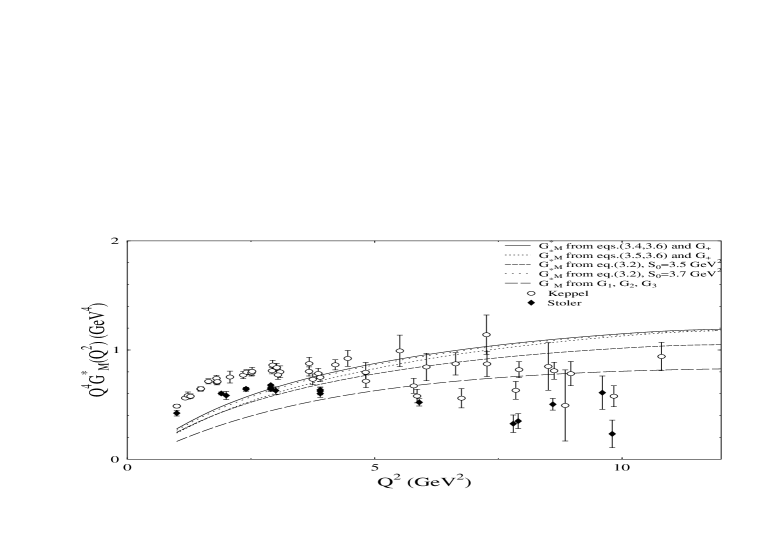
FIG. 3.: Form factor $G_{M}^{*}(Q^{2})$.

$$\langle 3/2|\Gamma|1,-1/2\rangle\sim(G_{M}^{*}+G_{E}^{*})$$ (3.8)

violates the helicity conservation requirement for the hard subprocess amplitude. In other words, the pQCD prediction is that $(G_{M}^{*}+G_{E}^{*})$ behaves asymptotically like $1/Q^{6}$, while each of $G_{M}^{*}$ and $G_{E}^{*}$ behaves like $1/Q^{4}$. As a result, asymptotically $G_{E}^{*}\sim-G_{M}^{*}$. However, we consider here only the soft contribution generated by the Feynman mechanism for which the helicity conservation arguments are not applicable, and asymptotically all soft terms fall like $1/Q^{6}$ or faster. Thus, for the soft term, there are no a priori grounds to expect that $G_{E}^{*}\sim-G_{M}^{*}$. The smallness of $G_{E}^{*}(Q^{2})/G_{M}^{*}(Q^{2})$, dictated by the local duality calculation, strongly contrasts with the pQCD-based expectation that $G_{E}^{*}(Q^{2})\sim-G_{M}^{*}(Q^{2})$, and this allows for an experimental discrimination between the two competing mechanisms. It should be noted, however, that $G_{E}^{*}(Q^{2})$ is obtained in our calculation as a small difference between two large combinations $G^{(+)}(Q^{2})$ and $G^{(-)}(Q^{2})$, both dominated by $G_{M}^{*}(Q^{2})$. Hence, even a relatively small uncertainty in either of these combinations (which is always there, since the local duality gives only approximate estimates) can produce a rather large relative uncertainty in the values of $G_{E}^{*}$.

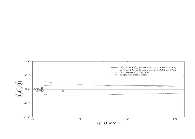
FIG. 4.: Ratio of form factors $G_{E}^{*}(Q^{2})$ and $G_{M}^{*}(Q^{2})$. Experimental data were taken from ref.[31] and the point at $3.2\,GeV^{2}$ from ref.[32].

Experimental points for $G_{M}^{*}(Q^{2})$ shown in Fig.3 were taken from the results for the $G_{T}(Q^{2})$ form factor obtained from the analyses of inclusive data [26], [30]. Since the local duality gives a very small value for the ratio $(G_{E}^{*}/G_{M}^{*})^{2}$, calculating the data points for $G_{M}^{*}(Q^{2})$ from $G_{T}(Q^{2})$, we neglected the $G_{E}^{*}$ term in eq.(2.18). One can see that, in the $Q^{2}\raisebox{-0.86108pt}{$\stackrel{{\scriptstyle\textstyle>}}{{\raisebox{-2.58334pt}[0.0pt][0.0pt]{$\sim$}}}$}3\,GeV^{2}$ region, the local duality predictions $G_{M}^{*}(Q^{2})$ are close in magnitude to the results of the recent analysis [30]. Our main conclusion is thus that the soft term is sufficiently large to play the dominant role at accessible energies.

The magnetic form factor $G_{M}^{*}(Q^{2})$ can also be obtained from the “contaminated” duality relation (3.2). If one takes the basic duality interval $S_{0}=3.5\,GeV^{2}$, the resulting values of $G_{M}^{*}(Q^{2})$ (Fig.3) are somewhat smaller than those obtained by combining the results for $G^{(+)}(Q^{2})$ and $G^{(-)}(Q^{2})$. Since the spin-1/2 states also contribute to the trace of $T_{\mu\nu}$, the duality interval in this case can be different from the basic value. In fact, taking $S_{0}=3.7\,GeV^{2}$ in eq.(3.2), we get a curve for $G_{M}^{*}(Q^{2}$ (Fig.3) essentially coinciding with those obtained from the sum of $G^{(+)}(Q^{2})$ and $G^{(-)}(Q^{2})$.

D $G_{2}(Q^{2})$ and $G_{3}(Q^{2})$

Using eq.(2.27) and applying the local duality prescription to the invariant amplitudes related to the structures $q_{\mu}p_{\nu}[\hat{p},\hat{q}]\gamma_{5}$ and $q_{\mu}q_{\nu}[\hat{p},\hat{q}]\gamma_{5}$, we get the following expressions for the $G_{2}(Q^{2})$ and $G_{3}(Q^{2})$ form factors:

$$G_{2}(Q^{2})=\left(1-Q^{2}\frac{d}{dQ^{2}}\right)\frac{d}{dQ^{2}}F(s_{0},S_{0},Q^{2})$$ (3.9)

$$G_{3}(Q^{2})-\frac{1}{2}G_{2}(Q^{2})=Q^{2}\left(\frac{d}{dQ^{2}}\right)^{3}\int_{0}^{S_{0}}F(s_{0},s_{2},Q^{2})ds_{2}.$$ (3.10)

As noted earlier, the second of these relations may be not very accurate. Still, using the explicit expressions (2.14-2.17) for $G_{E}^{*},G_{M}^{*},G_{C}^{*}$ in terms of $G_{1},G_{2},G_{3}$ and combining eqs.(3.9),(3.10) with the results for $G_{1}(Q^{2})$ obtained previously, we get an alternative way of calculating $G_{M}^{*}(Q^{2})$ and $G_{E}^{*}(Q^{2})$. The results are shown on Figs.3 and 4. One can see that the $G_{M}^{*}(Q^{2})$ form factor obtained in this way is a factor 1.5 smaller than that given by combining the results for $G_{-}(Q^{2})$ and $G_{+}(Q^{2})$. The deviation from previous results is even more drastic for $G_{E}^{*}(Q^{2})$. In this case, the new curve for $G_{E}^{*}(Q^{2})/G_{M}^{*}(Q^{2})$ has the sign opposite to that of the curves based on $G_{-}(Q^{2})$ and $G_{+}(Q^{2})$. However, as pointed out above, $G_{E}^{*}(Q^{2})$ is obtained in our calculation as a small net result of cancellations between large contributions dominated by $G_{M}^{*}(Q^{2})$, and the errors for a small form factor extracted in this way may be larger than its values. Still, the new curve is consistent with the old ones in the sense that the predicted ratio $|G_{E}^{*}(Q^{2})/G_{M}^{*}(Q^{2})|$ is small again. In this situation, we restrict ourselves to a conservative statement that the local quark-hadron duality indicates that the electric form factor $G_{E}^{*}(Q^{2})$ is small compared to $G_{M}^{*}(Q^{2})$ in the whole experimentally accessible region, without insisting on a specific curve (or even sign) for $G_{E}^{*}(Q^{2})$.

E $G_{C}(Q^{2})$

The quadrupole (Coulomb) form factor $G_{C}^{*}(Q^{2})$ can be calculated from the expression (2.28) for the contracted amplitude $p_{\nu}T_{\mu\nu}$:

$$G_{C}^{*}(Q^{2}) = \frac{8m}{3(M+m)}\left[-\frac{\partial}{\partial Q^{2}}\int_{0}^{S_{0}}F(s_{0},s_{2},Q^{2})\,ds_{2}-\frac{Q^{2}}{4}\left(\frac{\partial}{\partial Q^{2}}\right)^{2}\int_{0}^{s_{0}}F(s_{1},S_{0},Q^{2})\,ds_{1}\right.$$ (3.12)

$$\left.+\frac{1}{2}\left(\frac{\partial}{\partial Q^{2}}\right)^{2}\left(1+\frac{\partial}{\partial Q^{2}}\right)\int_{0}^{s_{0}}ds_{1}\int_{0}^{S_{0}}F(s_{1},s_{2},Q^{2})\,ds_{2}\right]\,.$$

FIG. 5.: Ratio $G_{C}^{*}(Q^{2})/G_{M}^{*}(Q^{2})$.

Again, $G_{C}^{*}(Q^{2})$ is essentially smaller than $G_{M}^{*}(Q^{2})$ (see Fig.5). Furthermore, eq.(3.12) predicts that, for large $Q^{2}$, the quadrupole form factor $G_{C}^{*}(Q^{2})$ has an extra $1/Q^{2}$ suppression compared to $G_{M}^{*}(Q^{2})$. In fact, if the duality intervals were equal, $s_{0}=S_{0}$, the suppression would be even stronger, namely, by two powers of $1/Q^{2}$.

The curve for $G_{C}^{*}(Q^{2})$ obtained from the expressions for $G_{1},G_{2},G_{3}$ gives somewhat larger (and opposite in sign) values for the ratio $G_{C}^{*}(Q^{2})/G_{M}^{*}(Q^{2})$, but the difference between the two results can be attributed again to the uncertainty in the values of large form factors $G_{1},G_{2},G_{3}$.

IV Conclusions

In this paper, we used the local quark-hadron duality approach to estimate the purely nonperturbative soft contribution to the $\gamma^{*}p\to\Delta^{+}$ transition form factors. Our results can be also applied to the $\gamma^{*}n\to\Delta^{0}$ transition: $G_{M,E,C}^{\gamma^{*}n\to\Delta^{0}}(Q^{2})=-G_{M,E,C}^{\gamma^{*}p\to\Delta^{+}}(Q^{2})$, $i.e.$ the only difference is the sign of the relevant form factors. The large-$Q^{2}$ behaviour of the soft contribution is governed by the Feynman mechanism which formally has an extra $1/Q^{2}$ suppression in the region of asymptotically large $Q^{2}$. However, our estimates for the effective form factor $G_{T}(Q^{2})$ are close to those obtained from a recent analysis of inclusive data [30]. This means that the data can be described without a sizable contribution from the hard-scattering mechanism. We picked out several Lorentz structures which appear in the decomposition of the basic three-point amplitude and observed a satisfactory agreement between the results obtained from different invariant amplitudes. All our estimates indicate that the transition is dominated by the magnetic form factor $G_{M}^{*}(Q^{2})$, with electric $G_{E}^{*}(Q^{2})$ and quadrupole $G_{C}^{*}(Q^{2})$ form factors being small compared to $G_{M}^{*}(Q^{2})$ for all experimentally accessible momentum transfers. This opens a possibility for a direct experimental verification of the soft contribution dominance in future exclusive measurements of the $\gamma^{*}N\to\Delta$ transition form factors at CEBAF.

V Acknowledgements

We are most grateful to V.D.Burkert, C.E.Carlson, N.Isgur and P.Stoler for discussions which strongly motivated this investigation. We thank C. Keppel for providing us with the results of her analysis and L.L.Frankfurt, J.L. Goity, F.Gross, I.V.Musatov, M.J.Musolf, R.Schiavilla, M.A. Strikman and W.J. van Orden for interest in this work and critical comments.

This work was supported by the US Department of Energy under contract DE-AC05-84ER40150.

A Parametric representation

To transform the amplitude $I_{\mu\nu}(x,y)$ (see eq.(2.4)) into the momentum representation, it is convenient to use the formula

$$\frac{1}{\pi^{4}}\int e^{ipx-iqy} \frac{d^{4}xd^{4}y}{(x-y)^{2l}y^{2m}x^{2n}}$$ (A.1)

$$= \frac{(-1)^{l+m+n+1}}{l!m!n!}\int_{0}^{\infty}\exp\left(\frac{\alpha p_{1}^{2}+\beta p_{2}^{2}+\gamma q^{2}}{4(\alpha\beta+\beta\gamma+\gamma\alpha)}\right)\frac{d\alpha^{l}d\beta^{m}d\gamma^{n}}{(\alpha\beta+\beta\gamma+\gamma\alpha)^{2}}$$ (A.2)

$$= \frac{(-1)^{l+m+n+1}}{4^{l+m+n-4}\,l!m!n!}\int_{0}^{\infty}e^{\tau_{1}p_{1}^{2}+\tau_{2}p_{2}^{2}+\tau_{3}q^{2}}\frac{d\tau_{1}^{l}d\tau_{2}^{m}d\tau_{3}^{n}}{(\tau_{1}\tau_{2}+\tau_{2}\tau_{3}+\tau_{3}\tau_{1})^{l+m+n-2}}$$ (A.3)

derived in ref.[37].

The numerator factors like $x_{\mu},y_{\mu}$ can be incorporated $via$

$$x_{\mu}\rightarrow-i\frac{\partial}{\partial p_{\mu}}\ \ ,\ \ y_{\mu}\rightarrow i\frac{\partial}{\partial q_{\mu}}\ .$$ (A.4)

Now, using eqs.(A.3,A.4), we get

$$I_{\mu\nu}(p,q)=\frac{(e_{u}-e_{d})}{16\pi^{4}}\int_{0}^{\infty}\sum_{i}a^{i}_{\mu\nu}(p,q)f^{i}(\tau_{1},\tau_{2},\tau_{3})e^{\tau_{1}p_{1}^{2}+\tau_{2}p_{2}^{2}+\tau_{3}q^{2}}\frac{d\tau_{1}d\tau_{2}d\tau_{3}}{(\tau_{1}\tau_{2}+\tau_{2}\tau_{3}+\tau_{3}\tau_{1})^{5}},$$ (A.5)

where

$$\sum_{i}a^{i}_{\mu\nu}(p,q)f^{i}(\tau_{1},\tau_{2},\tau_{3})=g_{\mu\nu}[p,q]\left(3\tau_{1}\tau_{2}\tau_{3}^{2}(\tau_{1}\tau_{2}+\tau_{2}\tau_{3}+\tau_{3}\tau_{1})-\tau_{1}\tau_{2}^{2}\tau_{3}^{3}\right)$$ (A.6)

$$+q_{\mu}[\gamma_{\nu},p]\left(4\tau_{1}\tau_{2}\tau_{3}^{3}(\tau_{1}+\tau_{2})-\tau_{1}^{2}\tau_{2}\tau_{3}^{3}\right)-3q_{\mu}[\gamma_{\nu},q]\tau_{1}^{2}\tau_{2}\tau_{3}^{3}$$ (A.7)

$$+2q_{\mu}p_{\nu}[p,q]\tau_{1}^{2}\tau_{2}^{2}\tau_{3}^{3}+2q_{\mu}q_{\nu}\ [p,q]\tau_{1}^{2}\tau_{2}\tau_{3}^{4}+\ldots\,,$$ (A.8)

and only the structures containing $g_{\mu\nu}$ or $q_{\mu}$ are displayed explicitly.

For the projection $p_{\nu}I_{\mu\nu}(p,q)$ used in the calculation of the $G_{C}^{*}(Q^{2})$ form factor, we have:

$$p_{\nu}I_{\mu\nu}(p,q)=p_{\nu}\int e^{ipx-iqy}I_{\mu\nu}(x,y)d^{4}xd^{4}y=i\int e^{ipx-iqy}\frac{\partial}{\partial x_{\nu}}I_{\mu\nu}(x,y)d^{4}xd^{4}y,$$ (A.9)

where

$$\frac{\partial}{\partial x_{\nu}}I_{\mu\nu}=\frac{6(e_{u}-e_{d})}{\pi^{8}}\left\{x_{\mu}\hat{y}\hat{x}\left(\frac{8}{x^{8}(x-y)^{4}y^{4}}+\frac{16}{x^{10}(x-y)^{4}y^{2}}-\frac{16}{x^{10}(x-y)^{2}y^{4}}\right)\right.$$ (A.14)

$$\left.+\gamma_{\mu}\hat{x}\left(-\frac{1}{x^{6}(x-y)^{4}y^{4}}-\frac{4}{x^{8}(x-y)^{4}y^{2}}+\frac{5}{x^{8}(x-y)^{2}y^{4}}+\frac{8}{x^{10}(x-y)^{2}y^{2}}\right)\right.$$

$$\left.+\gamma_{\mu}\hat{y}\left(\frac{2}{x^{6}(x-y)^{4}y^{4}}+\frac{7}{x^{8}(x-y)^{4}y^{2}}-\frac{7}{x^{8}(x-y)^{2}y^{4}}\right)\right.$$

$$\left.+x_{\mu}\left(-\frac{4}{x^{6}(x-y)^{4}y^{4}}-\frac{4}{x^{8}(x-y)^{4}y^{2}}+\frac{4}{x^{8}(x-y)^{2}y^{4}}\right)\right.$$

$$\left.+y_{\mu}\left(-\frac{-12}{x^{8}(x-y)^{4}y^{2}}+\frac{12}{x^{8}(x-y)^{2}y^{4}}\right)-\frac{4y_{\mu}\hat{y}\hat{x}}{x^{8}(x-y)^{4}y^{4}}\right\}\,.$$

In the momentum representation, this gives

$$p_{\nu}I_{\mu\nu}(p,q)=q_{\mu}[\hat{q},\hat{p}]\frac{e_{u}-e_{d}}{8\pi^{4}}\int\tau_{1}(\tau_{1}-\tau_{2})(\tau_{2}+\tau_{3})\tau_{3}^{3}$$ (A.15)

$$e^{\tau_{1}p_{1}^{2}+\tau_{2}p_{2}^{2}+\tau_{3}q^{2}}\,\frac{d\tau_{1}d\tau_{2}d\tau_{3}}{(\tau_{1}\tau_{2}+\tau_{2}\tau_{3}+\tau_{3}\tau_{1})^{5}}+...\,,$$ (A.16)

where only the term related to $G_{C}^{*}(Q^{2})$ was retained. For the amplitude Tr$\{I_{\mu\nu}\}$, we have:

$${\rm Tr}\{I_{\mu\nu}(x,y)\}=-\frac{6(e_{u}-e_{d})\left(4i\varepsilon^{\mu\nu\alpha\beta}y_{\alpha}x_{\beta}\right)}{\pi^{8}x^{6}(x-y)^{4}y^{4}}\,,$$ (A.17)

or, in the momentum representation:

$${\rm Tr}\{I_{\mu\nu}(p,q)\}=-\frac{3(e_{u}-e_{d})}{16\pi^{4}}\left(4i\varepsilon^{\mu\nu\alpha\beta}q_{\alpha}p_{\beta}\right)\int_{0}^{\infty}\tau_{1}\tau_{2}\tau_{3}^{2}\,e^{\tau_{1}p_{1}^{2}+\tau_{2}p_{2}^{2}+\tau_{3}q^{2}}\frac{d\tau_{1}d\tau_{2}d\tau_{3}}{(\tau_{1}\tau_{2}+\tau_{2}\tau_{3}+\tau_{3}\tau_{1})^{4}}\,{}.$$ (A.18)

B Calculation of spectral densities

To find the spectral densities corresponding to invariant amplitudes $T_{i}(p_{1}^{2},p_{2}^{2},Q^{2})$, it is convenient to start with the SVZ-transform of the double dispersion relation (2.19)

$${\cal B}(p_{1}^{2}\to M_{1}^{2}){\cal B}(p_{2}^{2}\to M_{2}^{2})T_{i}(p_{1}^{2},p_{2}^{2},Q^{2})\equiv\Phi_{i}(M_{1}^{2},M_{2}^{2},Q^{2})$$ (B.1)

$$=\frac{1}{\pi^{2}}\int_{0}^{\infty}\rho_{i}(s_{1},s_{2},Q^{2})\,e^{-s_{1}/M_{1}^{2}-s_{2}/M_{2}^{2}}ds_{1}ds_{2}\,,$$ (B.2)

where ${\cal B}(p^{2}\to M^{2})$ is the SVZ-operation [9] defined by

$${\cal B}(p^{2}\to M^{2})\frac{1}{s-p^{2}}=e^{-s/M^{2}}.$$ (B.3)

Explicit expressions for the SVZ-transforms $\Phi_{i}(M_{1}^{2},M_{2}^{2},Q^{2})$ can be easily obtained by applying the ${\cal B}$-operation to the parametric representation (A.3) using the formula [22]

$${\cal B}(p^{2}\to M^{2})\,e^{xp^{2}}=\delta(x-1/M^{2}).$$ (B.4)

Let us consider first the basic integral

$$J_{0}^{(4)}(p_{1}^{2},p_{2}^{2},q^{2})=\int_{0}^{\infty}\tau_{1}\tau_{2}\tau_{3}^{2}\,e^{\tau_{1}p_{1}^{2}+\tau_{2}p_{2}^{2}+\tau_{3}q^{2}}\frac{d\tau_{1}d\tau_{2}d\tau_{3}}{(\tau_{1}\tau_{2}+\tau_{2}\tau_{3}+\tau_{3}\tau_{1})^{4}}$$ (B.5)

corresponding to the spectral density $\rho_{0}(s_{1},s_{2},Q^{2})$ of the amplitude (A.18) given by the trace of $T_{\mu\nu}$. Applying the double SVZ-transformation (B.2), we obtain the equation

$$J_{0}^{(4)}(\tau_{1},\tau_{2};Q^{2})\equiv\int_{0}^{\infty}\frac{\tau_{1}\tau_{2}\tau_{3}^{2}}{(\tau_{1}\tau_{2}+\tau_{2}\tau_{3}+\tau_{3}\tau_{1})^{4}}\,e^{-\tau_{3}Q^{2}}d\tau_{3}$$ (B.6)

$$=\frac{1}{\pi^{2}}\int_{0}^{\infty}\rho_{0}(s_{1},s_{2},Q^{2})\,e^{-\tau_{1}s_{1}-\tau_{2}s_{2}}ds_{1}ds_{2},$$

where, according to eq.(B.4), $\tau_{1},\tau_{2}$ are now related to the SVZ-Borel parameters: $\tau_{1}=1/M_{1}^{2}$ and $\tau_{2}=1/M_{2}^{2}$.

This spectral density has been calculated in refs.[22],[37]:

$$\frac{1}{\pi^{2}}{\rho_{0}(s_{1},s_{2},Q^{2})}=\frac{Q^{2}}{24\kappa^{3}}(\kappa-(s_{1}+s_{2}+Q^{2}))^{2}(2\kappa+s_{1}+s_{2}+Q^{2})$$ (B.7)

$$=\frac{2}{3}Q^{2}s_{1}^{2}s_{2}^{2}\frac{2\kappa+s_{1}+s_{2}+Q^{2}}{\kappa^{3}(\kappa+(s_{1}+s_{2}+Q^{2}))^{2}}$$ (B.8)

where $\kappa=\sqrt{(s_{1}+s_{2}+Q^{2})^{2}-4s_{1}s_{2}}$.

The most economic way to calculate the spectral densities of other amplitudes is to express them in terms of the fundamental density $\rho_{0}(s_{1},s_{2},Q^{2})$. To do this, one should relate the relevant integrals to the basic integral (B.5). According to eqs. (A.8), (A.16), all these integrals have the form

$$J_{j}(p_{1}^{2},p_{2}^{2},q^{2})=\int_{0}^{\infty}g_{j}(\tau_{1},\tau_{2},\tau_{3})\tau_{3}^{3}\,e^{\tau_{1}p_{1}^{2}+\tau_{2}p_{2}^{2}+\tau_{3}q^{2}}\frac{d\tau_{1}d\tau_{2}d\tau_{3}}{(\tau_{1}\tau_{2}+\tau_{2}\tau_{3}+\tau_{3}\tau_{1})^{5}}$$ (B.9)

where $g_{j}(\tau_{1},\tau_{2},\tau_{3})$ in our case are some simple polynomials: $\tau_{1}^{2}\tau_{2}$, $\tau_{1}\tau_{2}^{2},$ $\tau_{1}^{2}\tau_{2}^{2},$ $\tau_{1}\tau_{2}\tau_{3}$ and $\tau_{1}^{2}\tau_{3}$.

After the double SVZ transformation, we have the equation

$$\int_{0}^{\infty}\frac{g_{j}(\tau_{1},\tau_{2},\tau_{3})\tau_{3}^{3}}{(\tau_{1}\tau_{2}+\tau_{2}\tau_{3}+\tau_{3}\tau_{1})^{5}}\,e^{-\tau_{3}Q^{2}}d\tau_{3}=\frac{1}{\pi^{2}}\int_{0}^{\infty}\rho_{j}(s_{1},s_{2},Q^{2})\,e^{-\tau_{1}s_{1}-\tau_{2}s_{2}}ds_{1}ds_{2}$$ (B.10)

where $\rho_{j}(s_{1},s_{2},Q^{2})$ is the relevant density and, again, $\tau_{1}=1/M_{1}^{2}$, $\tau_{2}=1/M_{2}^{2}$.

Further progress is based on the formula

$$J_{11}^{(5)}(\tau_{1},\tau_{2};Q^{2})\equiv\int_{0}^{\infty}\frac{\tau_{1}^{2}\tau_{2}^{2}\tau_{3}^{3}}{(\tau_{1}\tau_{2}+\tau_{2}\tau_{3}+\tau_{3}\tau_{1})^{5}}\,e^{-\tau_{3}Q^{2}}d\tau_{3}$$ (B.11)

$$=\frac{Q^{2}}{4}\int_{0}^{\infty}\frac{\tau_{1}\tau_{2}\tau_{3}^{4}}{(\tau_{1}\tau_{2}+\tau_{2}\tau_{3}+\tau_{3}\tau_{1})^{4}}\,e^{-\tau_{3}Q^{2}}d\tau_{3}\ .$$ (B.12)

The last integral looks very much like the basic integral $J_{0}^{(4)}(\tau_{1},\tau_{2};Q^{2})$ except for the two extra powers of $\tau_{3}$ in the numerator. However, an extra $\tau_{3}$ can be easily obtained by differentiating $J_{0}(\tau_{1},\tau_{2};Q^{2})$ with respect to $Q^{2}$. Hence,

$$J_{11}^{(5)}(\tau_{1},\tau_{2};Q^{2})=\frac{Q^{2}}{4}\left(\frac{\partial}{\partial Q^{2}}\right)^{2}J_{0}^{(4)}(\tau_{1},\tau_{2};Q^{2})\,,$$ (B.13)

or, in terms of densities

$$\rho_{11}(s_{1},s_{2};Q^{2})=\frac{Q^{2}}{4}\left(\frac{\partial}{\partial Q^{2}}\right)^{2}\rho_{0}(s_{1},s_{2};Q^{2}).$$ (B.14)

The notation $J_{11}^{(5)}$ implies that, compared to the basic integral $J_{0}^{(4)}(\tau_{1},\tau_{2};Q^{2})$, the integral $J_{11}(\tau_{1},\tau_{2};Q^{2})$ has one extra power of $\tau_{1}$, one extra power of $\tau_{2}$ in the numerator of its integrand and the 5th power of $(\tau_{1}\tau_{2}+\tau_{2}\tau_{3}+\tau_{3}\tau_{1})$ in the denominator. Since $\tau_{1}$ and $\tau_{2}$ do not participate in the $\tau_{3}$-integration, eq.(B.13) also gives

$$J_{01}^{(5)}(\tau_{1},\tau_{2};Q^{2})=\frac{Q^{2}}{4}\left(\frac{\partial}{\partial Q^{2}}\right)^{2}\frac{1}{\tau_{1}}J_{0}^{(4)}(\tau_{1},\tau_{2};Q^{2})\,$$ (B.15)

for the integral $J_{01}^{(5)}$ with $g(\tau_{1},\tau_{2},\tau_{3})=\tau_{1}\tau_{2}^{2}$. Note now, that the $1/\tau_{1}$ factor can be easily cancelled by performing integration by parts with respect to $s_{1}$ in the basic integral $J_{0}^{(4)}(\tau_{1},\tau_{2};Q^{2})$:

$$J_{0}^{(4)}(\tau_{1},\tau_{2};Q^{2})\equiv\int_{0}^{\infty}\rho_{0}(s_{1},s_{2},Q^{2})\,e^{-\tau_{1}s_{1}-\tau_{2}s_{2}}ds_{1}ds_{2}$$ (B.16)

$$=\tau_{1}\int_{0}^{\infty}\,e^{-\tau_{1}s_{1}-\tau_{2}s_{2}}ds_{1}ds_{2}\int_{0}^{s_{1}}\rho_{0}(s,s_{2},Q^{2})ds\ .$$ (B.17)

In terms of densities, this gives

$$\rho_{01}(s_{1},s_{2};Q^{2})=\frac{Q^{2}}{4}\left(\frac{\partial}{\partial Q^{2}}\right)^{2}\int_{0}^{s_{1}}\rho_{0}(s,s_{2};Q^{2})ds.$$ (B.18)

These and similar tricks can be applied to integrals with other forms of $g(\tau_{1},\tau_{2},\tau_{3})$ as well: each extra power of $\tau_{3}$ would produce an extra differentiation of $\rho_{0}(s_{1},s_{2};Q^{2})$ with respect to $Q^{2}$, while each missing power of $\tau_{1}$ or $\tau_{2}$ in the numerator (compared to $\tau_{1}^{2}\tau_{2}^{2}$) would result in an extra integration of $\rho_{0}(s_{1},s_{2};Q^{2})$ over $s_{1}$ or $s_{2}$, respectively.

REFERENCES

- [1] S.J. Brodsky and G.R. Farrar, Phys. Rev. Lett. 31 (1973) 1153.
- [2] R.P. Feynman, “Photon-Hadron Interaction”; W.A.Benjamin, Reading, Mass. (1972).
- [3] V.L. Chernyak and A.R. Zhitnitsky, JETP Lett. 25 (1977) 510; Yad. Fiz. 31 (1980) 1053.
- [4] A.V. Efremov and A.V. Radyushkin, Phys. Lett. B94 (1980) 245; Theor. Mat. Fiz. 42 (1980) 147.
- [5] G.P. Lepage and S.J. Brodsky, Phys. Lett. B87 (1979) 359; Phys. Rev. D22 (1980)
- [6] V.L. Chernyak and A.R. Zhitnitsky, Phys. Rep. 112 (1984) 173.
- [7] N. Isgur and C.H. Llewellyn-Smith, Nucl. Phys. B317 (1989) 526.
- [8] J. Bolz Z.Phys. C66 (1995) 267.
- [9] M.A. Shifman, A.I. Vainshtein and V.I. Zakharov, Nucl. Phys. B147 (1979) 385, 448.
- [10] S.V. Mikhailov and A.V. Radyushkin, Phys. Rev. D45 (1992) 1754.
- [11] A.V. Radyushkin, “Continuous advances in QCD”, ed. by A.V.Smilga, World Scientific, Singapore (1994) 238; hep-ph/9406237.
- [12] V.M. Braun and I.Filyanov, Z. Phys. C44 (1989) 157.
- [13] D.Daniel, R.Gupta and D.G.Richards, Phys. Rev. D43 (1991) 3715.
- [14] H.-J.Behrend et al. ( CELLO Collaboration), Z. Phys. C49 (1991) 401.
- [15] V.Savinov (CLEO-II collaboration), Contribution to the PHOTON95 conference (Sheffield, April 1995), hep-ex/9507005.
- [16] A.V. Radyushkin, In “Baryons ‘92”, ed. by M.Gai, World Scientific, Singapore (1993) 366.
- [17] V.M. Braun and I. Halperin, Phys. Lett. B328 (1994) 457.
- [18] B.L. Ioffe and A.V. Smilga, Phys. Lett. B114 (1982) 353.
- [19] V.A. Nesterenko and A.V. Radyushkin, Phys. Lett. B115 (1982) 410.
- [20] V.A. Nesterenko and A.V. Radyushkin, JETP. Lett. 39 (1984) 707.
- [21] A.P. Bakulev and A.V. Radyushkin, Phys. Lett. B271 (1991) 223.
-
[22]
V.A. Nesterenko and A.V. Radyushkin, Phys. Lett. 128B
(1983) 439;
Sov. J. Nucl. Phys. 39 (1984) 811. - [23] A.F. Sill et al. Phys. Rev. D48 (1993) 29.
- [24] P. Bosted et al. Phys. Rev. Lett. 68 (1992) 3841; Phys.Rev. D50 (1994) 5491.
- [25] G. Martinelli and C.T. Sachrajda, Phys. Lett. 217B (1989) 319.
- [26] P. Stoler, Phys. Rev. Lett. 66 (1991) 1003; Phys. Rev. D44 (1991) 73.
- [27] V.A.Matveev, R.M.Muradyan and A.N. Tavkhelidze, Lett. Nuovo Cim. 7 (1973) 719.
- [28] C.E. Carlson, Phys.Rev. D34 (1986) 2704.
- [29] N.G.Stefanis and M.Bergmann, Phys. Lett. B304 (1993) 24.
- [30] C. Keppel, Ph.D. Thesis, The American University (1995); also in: Workshop on CEBAF at Higher Energies, ed. by N. Isgur and P. Stoler, CEBAF, Newport News (1994) 237.
- [31] V.D. Burkert, in: Few-Body Problems in Physics, ed. by F. Gross, AIP Conference Proceedings 334 (1995) 127.
- [32] V.D. Burkert and L. Elouadrhiri, preprint CEBAF-PR-95-001, Newport News (1995).
- [33] B.L. Ioffe, Nucl. Phys. 188B (1981) 317.
-
[34]
J. Mathews, Phys. Rev. 137 (1965) B444;
H.F. Jones and M.D. Scadron, Annals of Physics 81 (1973) 1. - [35] P. Stoler, Phys. Reports 226 (1993) 103.
- [36] B.L. Ioffe and A.V. Smilga, JETP Lett 37 (1983)298 .
- [37] V.M. Belyaev and I.I. Kogan, preprint ITEP-29, Moscow (1984); Int.J.Mod.Phys. A8 (1993)153.
- [38] I.I. Balitsky, V.M. Braun, A.V. Kolesnichenko, Nucl.Phys. B312 (1989) 509.
- [39] V.M. Belyaev and B.L. Ioffe, Sov.Phys.JETP 56 (1982) 493.