EFI-95-22

CERN-TH/95-145

ENSLAPP-A-523/95

ISN 95-07

ITKP 95-17

hep-ph/9506315

SPACINGS OF QUARKONIUM LEVELS

WITH THE SAME PRINCIPAL QUANTUM NUMBER

Aaron K. Grant and Jonathan L. Rosner

Enrico Fermi Institute and Department of Physics

University of Chicago, Chicago, IL 60637

André Martin

Theory Group, CERN, 1211-CH-Geneva 23, Switzerland

and

Laboratoire de Physique Théorique ENSLAPP

Groupe d’Annecy, LAPP, B. P. 110

F-74941 Annecy-le-Vieux, France

Jean-Marc Richard

Institut de Sciences Nucléaires–CNRS-IN2P3

Université Joseph Fourier

53, avenue des Martyrs, 38026 Grenoble Cedex, France

and

Institut für Theoretische Kernphysik

Rheinische Friedrich-Wilhelms Universität

Nu$\ss$allee 14-16, D-53115 Bonn, Germany

Joachim Stubbe

Département de Physique Théorique, Université de Genève

CH-1211 Genève 4, Switzerland

ABSTRACT

The spacings between bound-state levels of the Schrödinger equation with the same principal quantum number $N$ but orbital angular momenta $\ell$ differing by unity are found to be nearly equal for a wide range of power potentials $V=\lambda r^{\nu}$, with $E_{N\ell}\approx F(\nu,N)-G(\nu,N)\ell$. Semiclassical approximations are in accord with this behavior. The result is applied to estimates of masses for quarkonium levels which have not yet been observed, including the 2P $c\bar{c}$ states and the 1D $b\bar{b}$ states.

I. INTRODUCTION

The properties of heavy quarkonium ($c\bar{c}$ and $b\bar{b}$) levels have provided useful insights into the nature of the strong interactions. At short distances these interactions appear to be characterized by a Coulombic potential associated with asymptotically free single-gluon exchange [1], while at large distances the interquark force is consistent with a constant, corresponding to a separation energy increasing linearly with distance [2]. An effective power potential $V\sim r^{\nu}$, with $\nu$ close to zero, provides a useful interpolation between these two regimes for $c\bar{c}$ and $b\bar{b}$ levels when the interquark separation ranges between about 0.1 and 1 fm [3].

Charmonium ($c\bar{c}$) levels have been identified up to the fourth or fifth S-wave, the first P-wave, and the first D-wave excitation. (We are ignoring fine structure and hyperfine structure for the moment.) Six S-wave levels and two P-wave levels have been found in the upsilon ($b\bar{b}$) family. Many additional levels are expected but have not yet been seen. There are some reasons of current interest for predicting their positions in a relatively model-independent manner. For example:

(1) It has been suggested [4, 5] that, depending on its exact mass, the second charmonium P-wave level (which we shall denote as $\chi_{c}^{\prime}(2P)$) could play a role in the hadronic production of the $\psi^{\prime}(2S)$ state.

(2) The first D-wave level of the $b\bar{b}$ system, which we shall call $\Upsilon(1D)$, may be accessible to experiments of improved sensitivity at the CLEO detector, both in direct production of the ${}^{3}D_{1}$ states via the $e^{+}e^{-}$ channel and through electromagnetic transitions from the $\Upsilon(3S)$ state [6].

Explicit calculations in nonrelativistic quark models of the masses of the $\chi_{c}^{\prime}(2P)$ and $\Upsilon(1D)$ states have tended to have very small spreads [6, 7]. Any interquark potential which reproduces the known quarkonium levels is well-enough determined to leave little room for variation in predictions of these levels. However, in the course of examining these predictions within the context of power potentials $V=\lambda r^{\nu}$, with $\lambda\nu>0$, we were struck by a curious feature: The spacings between levels with the same principal quantum number but orbital angular momenta differing by unity are nearly identical for a wide range of values of $\nu$.

The principal quantum number $N$ is that which labels nonrelativistic Coulomb energy levels through the Balmer formula $E_{N\ell}\propto-1/N^{2}$. It is related to the radial quantum number $n_{r}$ and the orbital angular momentum $\ell$ via $N=n_{r}+\ell~{}(n_{r}=1,2,3,\ldots)$, where $n_{r}-1\equiv n$ corresponds to the number of nodes of the radial wave function between $r=0$ and $r=\infty$. Our result amounts to a formula for levels $E_{N\ell}$ linear in $\ell$ for a given $N$:

$$E_{N\ell}=F(\nu,N)-G(\nu,N)\ell$$ (1)

with $G(\nu,N)>0$ for $\nu>-1$ in accord with a much more general result which specifies the order of levels for fixed $N$ as a function of $\ell$ [8]. This general result is that $G$ is positive for any potential whose Laplacian is positive everywhere outside the origin. We investigate this general case first in Section II, turning to the special case of power potentials in Sec. III. We apply the results to specific quarkonium cases in Sec. IV, while Sec. V summarizes. Some proofs of identities are given in three appendices.

II. POTENTIALS WITH POSITIVE LAPLACIAN

We consider the Schrödinger equation in appropriate dimensionless units ($\hbar=2\mu=1$, where $\mu$ is the reduced mass), for a spherically symmetric potential $V(r)$:

$$[-\Delta+V(r)]\Psi_{N\ell}({\bf r})=E_{N\ell}\Psi_{N\ell}({\bf r}){}~{}~{}.$$ (2)

Potentials with positive Laplacian $\Delta V>0$ play a special role in quarkonium physics. First, all potentials used to fit the $b\bar{b}$ and $c\bar{c}$ spectrum have positive Laplacian (except for spurious pathologies when one expands the potential in powers of the strong coupling constant at a given scale). It is in fact very natural to take potentials with positive Laplacian because this property is a kind of expression of asymptotic freedom: If we say that the force between a quark and an antiquark is $F=-\alpha(r)/r^{2}$, asymptotic freedom requires that $\alpha(r)$ be an increasing function of $r$. Writing $F=-dV/dr$, saying that $\alpha(r)$ increases is equivalent to

$$\frac{d}{dr}r^{2}\frac{dV}{dr}>0~{}~{}~{},$$ (3)

which means that $V$ has a positive Laplacian. If this is the case we have [8], for a given multiplet,

$$E_{N,\ell-1}>E_{N,\ell}>E_{N,\ell+1}$$ (4)

for $N\geq 3,~{}\ell\geq 1$.

Very soon after the discovery of this property, Baumgartner [9] proved the following theorem:

Define

$$R_{N,\ell}\equiv\frac{E_{N,\ell-1}-E_{N,\ell}}{E_{N,\ell}-E_{N,\ell+1}}{}~{}~{}.$$ (5)

Then

$$R_{N,\ell}\geq\frac{\ell}{\ell+1}\frac{N^{2}-(\ell+1)^{2}}{N^{2}-\ell^{2}}~{}~{}~{},$$ (6)

if $V=-(1/r)+\lambda v$, with $\Delta v\geq 0,~{}\lambda$ sufficiently small. Notice that the right-hand side of (6) is always less than unity. So (6) holds for perturbations of a Coulomb potential. It is not known if this inequality also holds outside the perturbative regime. Our belief is that it does hold, but the proof must be rather complex. The perturbative proof is based on the equation

$$\ell\alpha^{2}_{\ell-1}(E_{N,\ell-1}-E_{N,\ell})-(\ell+1)\alpha^{2}_{\ell}(E_{N,\ell}-E_{N,\ell+1})$$

$$=\frac{2\ell+1}{2}\int_{0}^{\infty}\Delta V(r)u_{N,\ell}^{2}dr~{}~{}~{}$$ (7)

where $u_{N,\ell}$ is a pure Coulomb wave function, and

$$4\alpha_{\ell}^{2}\equiv(\ell+1)^{-2}-N^{-2}~{}~{}~{}.$$ (8)

For $\Delta V>0$, the inequality (6) follows from (7) and (4). In fact, inequality (6) would also hold for a potential with purely negative Laplacian, since both (7) and (4) are reversed. The proof of (7) will be given in Appendix A. What is important is that this equation shows that Baumgartner’s result [9] cannot be improved, because it is saturated by a potential $v$ whose Laplacian has its support concentrated at the zeroes of $u_{n,\ell}$. Such a potential is easy to construct: It is made of piecewise shifted Coulomb potentials. The resulting overall potential is not concave, but can be made so by a correction of order $\lambda^{2}$ ($\lambda$ being the coefficient of $v$), for example by joining pairs of Coulomb segments by linear pieces tangent to each.

Even if one believes that (6) holds for non-perturbative situations, it is a rather disappointing result for practical applications. For instance, using the “particle physics” spectroscopic notation, we get

$$\frac{E_{3S}-E_{2P}}{E_{2P}-E_{1D}}>\frac{5}{16}~{}~{}~{},$$ (9)

while, as we shall see in the next section, this ratio can be very close to unity. On the other hand no improvement is possible. Even the very simple-minded potential $-(1/r)+\lambda r$ gives

$$\frac{E_{3S}-E_{2P}}{E_{2P}-E_{1D}}\to\frac{1}{2}$$ (10)

for $\lambda\to 0$, as shown in Appendix A, and we have checked numerically that for finite $\lambda$ this limit is approached smoothly. Therefore, to make progress, we should use a more restricted class of potential, the power potentials, which are known to give excellent fits of the heavy quark-antiquark spectra [3].

III. THE CASE OF POWER POTENTIALS

If $V(r)=\varepsilon(\nu)r^{\nu}$, where $\varepsilon(\nu)$ is the sign function and $-1<\nu<2$, one finds that $R_{N,\ell}$ is always very close to unity, to summarize briefly this section. The evidence comes from indications from semi-classical formulae valid for large quantum numbers, analytical investigations in the neighborhood of $\nu=-1$ and $\nu=2$, and explicit numerical calculations of energy levels for small quantum numbers, shown in Fig. 1. For the purpose of this figure, in order to obtain a smooth limit as $\nu\to 0$, we have represented the Schrödinger equation as

$$[-(1/2)\Delta+(r^{\nu}-1)/\nu]\Psi_{n_{r}\ell}({\bf r})=E_{n_{r}\ell}\Psi_{n_{r}\ell}({\bf r})~{}~{}~{},$$ (11)

and levels are labeled by the radial quantum number $n_{r}=N-\ell$ and the orbital angular momentum $\ell=(0,~{}1,~{}2,~{}3,~{}\ldots)=$(S, P, D, F, $\ldots$).

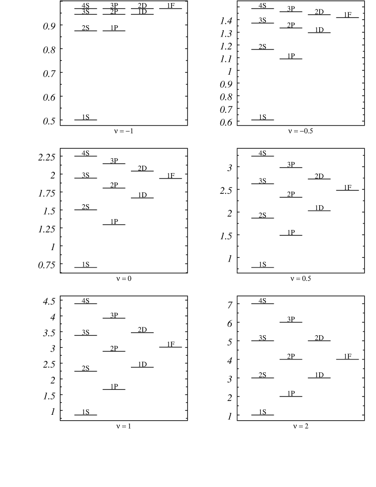
Figure 1: Energy levels in the Schrödinger equation (11) for several power potentials. Levels are labeled as described in the text.

For power potentials, semi-classical formulae are expected to hold for $N\to\infty$. However there are several regimes depending on whether $\ell$ stays small compared to $N$ or, on the contrary, $N-\ell$ stays small. In the latter case two of us [10] have shown that $E_{N,\ell}$ depends asymptotically only on the combination $N-\ell(1-\frac{1}{\sqrt{\nu+2}})$. In the former case $N\to\infty,~{}\ell$ finite, $E_{N,\ell}$ depends on $N-\frac{\ell}{2}$, the same combination as in the case of the harmonic oscillator, as shown by one of us and C. Quigg [11].

An exhaustive study of the various cases has been made by Feldman, Fulton, and Devoto [12]. We shall not give in the text the refined formulae obtained by these authors. (A further refinement is given in Appendix B.) We shall content ourselves with the leading terms. Here we express energies in terms of the number of nodes $n=n_{r}-1=N-\ell-1$ and the angular momentum $\ell$. We have, defining $E(N,\ell)\equiv\hat{E}(n,\ell)$, the following cases:

i) $\ell$ large, $n$ finite, $-2<\nu<\infty$:

$$\hat{E}(n,\ell)\sim\varepsilon(\nu)\left(\frac{|\nu|}{2}\right)^{-\frac{\nu}{\nu+2}}\left(1+\frac{\nu}{2}\right)$$

$$\times\left[\ell+\frac{1}{2}+\left(n+\frac{1}{2}\right)\sqrt{\nu+2}\right]^{\frac{2\nu}{\nu+2}}~{}~{}~{},$$ (12)

ii a) $n$ large, $\ell$ finite [11], $0<\nu<\infty$:

$$\hat{E}(n,\ell)\sim\left[2\sqrt{\pi}\frac{\Gamma(\frac{3}{2}+\frac{1}{\nu})}{\Gamma(1+\frac{1}{\nu})}\left(n+\frac{\ell}{2}-\frac{1}{4}\right)\right]^{\frac{2\nu}{\nu+2}}~{}~{}~{},$$ (13)

ii b) $n$ large, $\ell$ finite [11], $-2<\nu<0$:

$$\hat{E}(n,\ell)\sim-\left\{2|\nu|\sqrt{\pi}\frac{\Gamma(1-\frac{1}{\nu})}{\Gamma(-\frac{1}{2}-\frac{1}{\nu})}\left[n-\frac{1}{2}\left(\frac{1+\nu-2\ell}{2+\nu}\right)\right]\right\}^{\frac{2\nu}{\nu+2}}~{}~{}~{}.$$ (14)

These formulae exhibit very smooth behavior of the energies as functions of $n$ and $\ell$ and hence $N$ and $\ell$. Further support for the smoothness in $\ell$ for fixed $n$ is given in Appendix B, because $[\hat{E}(n,\ell)]^{\frac{\nu+2}{\nu}}$ is a “Herglotz” function of $(\ell+1/2)^{2}$ for $\nu\geq 0$.

In the case i), for $\ell\to\infty$, $n$ finite, one can write a systematic expansion of the energies in inverse powers of $\ell+\frac{1}{2}$ [13]. The first terms are

$$\hat{E}(n,\ell)=\left(\frac{|\nu|}{2}\right)^{\frac{2}{\nu+2}}\frac{2+\nu}{\nu}\left(\ell+\frac{1}{2}\right)^{\frac{2\nu}{\nu+2}}$$

$$\times\left\{1+\frac{2\nu}{\sqrt{\nu+2}}\frac{n+\frac{1}{2}}{\ell+\frac{1}{2}}+\frac{\nu(\nu-2)}{12(\nu+2)(\ell+\frac{1}{2})^{2}}\left[(11-\nu)(n+\frac{1}{2})^{2}+\frac{\nu+1}{12}\right]\right.$$

$$\left.+{\cal O}\left[\frac{\nu-2}{(\ell+\frac{1}{2})^{3}}\right]\right\}~{}~{}~{}.$$ (15)

Notice that this expression becomes exact for $\nu=2$. In Appendix B we show that (15) can be used to improve the Feldman–Fulton–Devoto [12] asymptotic expression for large $\ell$ in a rather impressive way. Eq. (15) yields the behavior of $R_{N,\ell}$ for $\ell\to\infty,~{}N-\ell$ finite:

$$R_{N,\ell}\simeq 1+\frac{(\nu-2)^{2}}{6(2\ell+1)}\frac{4-3\sqrt{\nu+2}-\nu}{(\nu+2)(\sqrt{\nu+2}+2)}$$

$$+{\cal O}\frac{(\nu-2)^{2}}{(2\ell+1)^{2}}~{}~{}~{}.$$ (16)

This expression shows that $R_{N,\ell}$ is indeed very close to unity for $-1\leq\nu\leq 2$, as long as $\ell\geq 2$.

Other limiting cases which can be treated analytically are $\nu\to-1$ and $\nu\to 2$, for arbitrary $n$ and $\ell$.

In the case $\nu\to-1$ it is sufficient to look at a perturbation of the Coulomb potential by a potential $\log(r)/r$, since

$$\lim_{\nu\to-1}\frac{r^{\nu}-r^{-1}}{\nu+1}=\frac{\log(r)}{r}{}~{}~{}.$$ (17)

Calculations presented in Appendix C give

$$R_{N,\ell}=\frac{N+\ell+1}{N+\ell}$$ (18)

for $\nu\to-1$.

In the case $\nu\to 2$, one should, similarly, take a perturbation $V=r^{2}\log r$. Then one gets the surprise that the terms of order $\nu-2$ vanish and

$$R_{N,\ell}\simeq 1+{\cal O}(\nu-2)^{2}~{}~{}~{}.$$ (19)

At this point, we see that it may be advantageous to replace Eq. (16) by

$$R_{N,\ell}\simeq 1+\frac{(\nu-2)^{2}}{6(N+\ell)}\frac{4-3\sqrt{\nu+2}-\nu}{(\nu+2)(\sqrt{\nu+2}+2)}~{}~{}~{},$$ (20)

which preserves the large-$\ell$ asymptotic behavior and agrees with (18) for $\nu\to-1$ and (16) for $\nu\to 2$.

All this fits perfectly into the numerical calculations presented in Figs. 2 and 3 for $(N=3,~{}\ell=1)$, $(N=4,~{}\ell=1)$, and $(N=4,~{}\ell=2)$. It is striking that the asymptotic formula (16) agrees quite well with the case in which $n$ is smallest and $\ell$ largest, i.e., $N=4,~{}\ell=2$. In particular the asymptotic formula reproduces the fact that $R-1$ is negative for $\sim 0.1<\nu<2$.

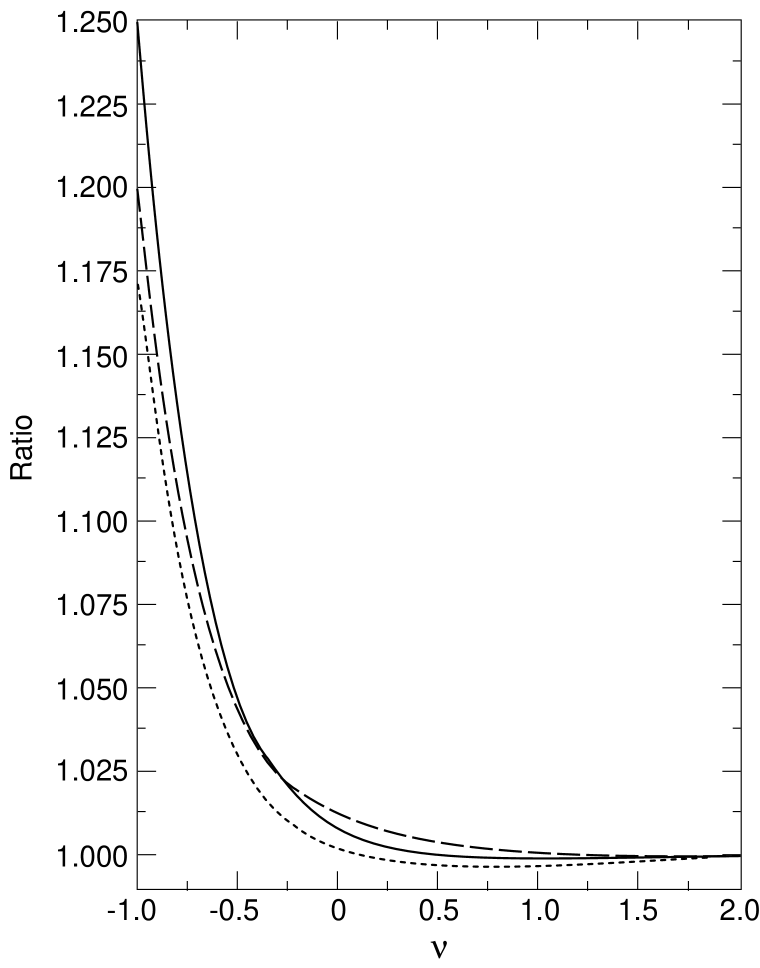
Figure 2: Ratios of spacings of levels with the same principal quantum number in power-law potentials $V(r)\sim r^{\nu}$ as a function of $\nu$. Solid curve: $[E(3S)-E(2P)]/[E(2P)-E(1D)]$; Dashed: $[E(4S)-E(3P)]/[E(3P)-E(2D)]$; Dotted: $[E(3P)-E(2D)]/[E(2D)-E(1F)]$. Here levels are labeled by $n_{r}$(S, P, D, F, $\ldots$), where $n_{r}=N-\ell$ is the radial quantum number.

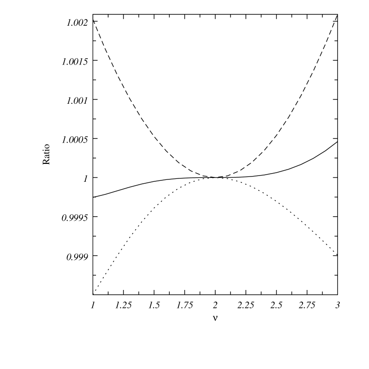
Figure 3: Ratios of spacings of levels with the same principal quantum number in power-law potentials $V(r)\sim r^{\nu}$ near $\nu=2$. Solid line: $[E(3S)-E(2P)]/[E(2P)-E(1D)]$; dashed line: $[E(4S)-E(3P)]/[E(3P)-E(2D)]$; dotted line: $[E(3P)-E(2D)]/[E(2D)-E(1F)]$. Levels are labeled as in Fig. 2.

For completeness let us indicate that for $\nu\to-2$, $R_{N,\ell}$ tends to $+\infty$. Notice first that, by scaling, $R_{N,\ell}$ is independent of the strength of the power potential. We can always take $V=-gr^{\nu}$ with $(\ell+\frac{1}{2})^{2}>g>(\ell-\frac{1}{2})^{2}$. Then $E_{N,\ell}$ and $E_{N,\ell+1}$ approach zero as $\nu\to-2$, while $E_{N,\ell-1}$ goes to $-\infty$. This is because, for a state of angular momentum $\ell$, the limit Hamiltonian is, for $\nu\to-2$,

$$H_{\rm lim}=-\frac{d^{2}}{dr^{2}}-\frac{1}{4r^{2}}+\frac{(\ell+\frac{1}{2})^{2}-g}{r^{2}}~{}~{}~{}.$$ (21)

The operator $-(d^{2}/dr^{2})-1/(4r^{2})$ is known to be positive, i.e., its expectation value for any reduced wave function vanishing at the origin is positive. Hence, if $g<(\ell+\frac{1}{2})^{2}$ the eigenvalues of $H_{\rm lim}$ are positive. However, for $0>\nu>-2$, the Hamiltonian has negative eigenvalues (in fact infinitely many!) and therefore the lowest eigenvalue has to go to zero for $\nu\to-2$. On the other hand for $g>(\ell+\frac{1}{2})^{2}$ it is known that $H_{\rm lim}$ is not lower-bounded, as can be seen by taking its expectation value with, for instance, a trial function $u=0$ for $r\leq R_{m}$, $(r-R_{m})^{\frac{1}{2}+\epsilon}(R_{M}-r)$ for $R_{m}<r<R_{M}$, 0 for $r\geq R_{M}$, and letting $R_{m}$ and $\epsilon$ go to zero. This not only proves that the ground state energy goes to $-\infty$, but all radial excitation energies do so as well. If $E_{n}$ is a finite limiting value of the energy level of the $n$th radial excitation, there is a sequence of energies and wave functions (defined by integration of the Schrödinger equation from infinity) which approaches the limit energy and wave function. Let $r_{k}$ be the first nonzero limit of a node for $\nu\to-2$. Then taking $r_{k-1}<R_{m}<R_{M}<r_{k}$, the energy corresponding to the interval $(R_{m},R_{M})$ with Dirichlet boundary conditions is higher than the one corresponding to $(r_{k-1},r_{k})$ and goes to $-\infty$, which is what we wanted to prove. If all nodes approach zero (which is in fact the case!) the proof obviously works, taking $R_{m}>r_{n}$.

The opposite extreme case is $\nu\to\infty$, i.e., the square well. Then the solutions of the Schrödinger equation are Bessel functions which can be approximated near their turning point by Airy functions. One gets, for instance,

$$\lim_{\ell\to\infty}R_{\ell+2,\ell}=\frac{|a_{3}|-|a_{2}|}{|a_{2}|-|a_{1}|}=0.818709\ldots~{}~{}~{},$$ (22)

where the $a_{i}$ are successive zeros of the Airy function.

IV. APPLICATIONS TO QUARKONIUM LEVELS

Realistic quarkonium potentials appear to have a power-law behavior $V\sim r^{\nu}$, [3], with $\nu$ not far from zero. For $-0.1<\nu<0.1$, $R_{3,1}$ is $1.007\pm 0.002$. Consequently, one can anticipate that energy levels with the same principal quantum number $N$ will depend nearly linearly on the orbital angular momentum $\ell$. We apply this result to two examples, one in charmonium and one in the upsilon family.

A. Charmonium $2P$ states

The $1P$ levels of charmonium were identified nearly 20 years ago in electric dipole transitions from the $\psi^{\prime}(2S)$ [14]. Recently they have been studied with great precision in proton-antiproton formation experiments [15]. Since they lie below threshold for decay to a pair of charmed mesons, they are quite narrow, facilitating their observation. The ${}^{3}P_{1}$ and ${}^{3}P_{2}$ levels, in particular, have substantial branching ratios to $\gamma+J/\psi$.

Recent interest has focused on the possibility that one or more charmonium $2P$ states may be narrow enough to have a substantial branching ratio to $\gamma+\psi^{\prime}(2S)$ [4, 5]. This suggestion is motivated by a production rate for $\psi^{\prime}(2S)$ in high-energy proton-antiproton collisions [16] which appears too high to be explained by conventional $QCD$ mechanisms. It then becomes of some interest to predict exactly where the $2P$ levels should lie. If the ${}^{3}P_{2}$ level lies sufficiently low, its decay to $D\overline{D}$, though kinematically allowed, will be suppressed by a large $\ell=2$ centrifugal barrier, so that its branching ratio to $\gamma+\psi^{\prime}(2S)$ could be non-negligible. The ${}^{3}P_{1}$ level cannot decay to $D\overline{D}$; it will be narrow if it lies below the $D\overline{D}^{*}$ threshold at 3.87 GeV. Reliable anticipation of the positions of the $2P$ levels may permit their discovery and study in the same low-energy direct-channel experiments which studied the $1P$ levels so successfully [15].

In order to anticipate the spin-weighted average $2P$ mass in charmonium, we need similar quantities for the $3S$ and $1D$ levels. The masses of the $3^{3}S_{1}$ and $1^{3}D_{1}$ states are quoted as $4040\pm 10$ and $3769.9\pm 2.5$ MeV, respectively [17]. Assuming hyperfine splittings in the $S$-wave levels to scale roughly as $1/N$ [3], and using the observed splitting of about 118 MeV between the $1^{3}S_{1}$ and $1^{1}S_{0}$ charmonium levels, we expect the spin-weighted average $3S$ mass to be about $4030\pm 10$ MeV. We must rely on a specific calculation [18] of fine structure to estimate the spin-weighted average $1D$ mass; the result is 3820 MeV. Thus we predict the spin-weighted $2P$ mass to lie around 3925 MeV. The prediction of a $2P$ level near the average of the $3S$ and $1D$ levels should be a feature of any smooth potential which reproduces charmonium and upsilon levels.

B. $1D$ states of the upsilon family

Electromagnetic transitions from the $\Upsilon(3S)$ to the $\chi_{b}^{\prime}(2P)$ levels, followed by transitions to the $\Upsilon(1D)$ levels and their subsequent decays, can give rise to characteristic photon spectra [6] to which the CLEO-II detector is uniquely sensitive. It is also possible for the CLEO-II detector to scan in energy for the $\Upsilon(1^{3}D_{1})$ level, whose leptonic width is expected to be one or two electron volts [18]. We expect the spin-weighted $\Upsilon(1D)$ mass to be the same distance below the spin-weighted $2P$ mass ($10.260\pm 0.001$ GeV) as the distance between this mass and the spin-weighted $3S$ mass. Here we do not know the hyperfine splitting between the observed $\Upsilon(3S)$ at $10.3553\pm 0.0005$ GeV and its spin-singlet partner. On the basis of the range of predictions for the $1S$ level and our assumption that hyperfine splittings scale as $1/N$, we estimate the hyperfine splitting in the $3S$ system to be 20 MeV, give or take a factor of 2, and hence the spin-averaged $3S$ level to lie at $10.349\pm 0.007$ GeV. Thus, we would expect the spin-averaged $\Upsilon(1D)$ level to lie around 10.17 GeV.

C. $2D$ and $3P$ states of the upsilon family

It may be possible to detect $2D$ upsilon levels through direct-channel $e^{+}e^{-}$ annihilation or hadronic production [6]. Potential models predict the spin-average of the $2D$ levels to lie around 10.44 GeV. Let us imagine that such a level has indeed been seen. Then, since the $\Upsilon(4S)$ state has a mass of about 10.58 GeV, the $3P$ level should lie midway between the two in a power-law potential, at 10.51 GeV. Since this is below $B\overline{B}$ threshold, the $3P$ level should be narrow, as has been noted previously [6]. This level, more easily produced in hadronic interactions than the $\Upsilon(3S)$, should then be able to populate the $3S$ level through electric dipole transitions, which may be detectable. Whichever level, $2D$ or $3P$, is seen first, our equal-spacing rule permits the other’s mass to be anticipated.

D. Possible sources of error in predictions

Explicit potential models predict a slightly lower $\Upsilon(1D)$ mass (ranging from 10.15 to 10.16 GeV) than our prediction of 10.17 GeV, as a consequence of the change in the effective power of the potential with distance. The $3S-2P$ splitting is more sensitive to the short-distance (more Coulomb-like) part of the potential, while the $2P-1D$ splitting is sensitive to longer-range effects, where the potential is expected to be closer to linear. For example, a typical Coulomb-plus-linear potential, such as $V(r)=-0.4/r+0.16r$, where $r$ is in GeV^-1, and $m_{b}=5$ GeV, implies $E(3S)-E(2P)$ around 15% less than $E(2P)-E(1D)$. To a lesser degree, such changes in effective power of the potential may be visible in deviations of the charmonium $2P$ and upsilon $3P$ masses from our predictions.

Coupled-channel effects can significantly distort predictions of potential models near pair production thresholds [19]. We expect such effects to be most significant in the anticipation of the charmonium $2P$ and upsilon $3P$ levels mentioned above, and less important for the upsilon $1D$ level.

V. SUMMARY

Interesting questions remain to be settled in quarkonium systems. The nonrelativistic Schrödinger equation continues to provide a useful guide to the properties of such systems, with power-law potentials $V\sim r^{\nu}$, $\nu\approx 0$, permitting rapid anticipation of charmonium and upsilon properties. We have shown that in a wide range of power-law potentials, energy levels characterized by the same principal quantum number are approximately linear in orbital angular momentum $\ell$, with a coefficient which is negative as long as $\nu>-1$. We have exhibited this behavior numerically, discussed the limiting cases of perturbations around the Coulomb and harmonic oscillator potentials, presented semiclassical results for the coefficient of $\ell$, and applied the results to the anticipation of several charmonium and upsilon levels which have yet to be observed.

ACKNOWLEDGMENTS

The authors would like to thank Jeanne Rostant and Luis Alvarez-Gaumé for organizing a celebration which was the starting point of this work. J. R. and A. M. respectively wish to thank the CERN Theory Group and Rockefeller University Physics Department for their hospitality. This work was supported in part by the United States Department of Energy under Contract No. DE FG02 90ER40560.

APPENDIX A: PROOF OF THE BAUMGARTNER THEOREM

AND EFFECT OF LINEAR PERTURBATIONS

The Schrödinger equation for a pure Coulomb potential is taken to be

$$H_{\ell}~{}u_{N,\ell}=\left(-\frac{d^{2}}{dr^{2}}+\frac{\ell(\ell+1)}{r^{2}}-\frac{1}{r}\right)u_{N,\ell}=-\frac{1}{4N^{2}}u_{N,\ell}~{}~{}~{}.$$

To prove the Baumgartner theorem, we let

$$\Delta_{N,\ell}=E_{N,\ell}-E_{N,\ell+1}~{}~{}~{}.$$

Then we have

$$\Delta_{N,\ell}=\int v\left(u^{2}_{N,\ell}-u^{2}_{N,\ell+1}\right)dr~{}~{}~{},$$

where the $u$’s are Coulomb wave functions. $u_{N,\ell}$ and $u_{N,\ell+1}$ are linked by raising and lowering operators:

$$A^{\pm}_{\ell}\equiv\pm\frac{d}{dr}-\frac{\ell+1}{r}+\frac{1}{2(\ell+1)}$$

$$A^{-}_{\ell}u_{N,\ell+1}=\alpha_{\ell}u_{N,\ell}~{}~{},~{}~{}~{}A^{+}_{\ell}u_{N,\ell}=\alpha_{\ell}u_{N,\ell+1}~{}~{}~{},$$

with $4\alpha^{2}_{\ell}\equiv(\ell+1)^{-2}-N^{-2}$. The the Coulomb Hamiltonian can be written as

$$H_{\ell}=A_{\ell}^{-}A_{\ell}^{+}-\frac{1}{4(\ell+1)^{2}}~{}~{}~{}.$$

Using these operators, one can transform $\Delta_{N,\ell}$ into

$$\alpha_{\ell}\Delta_{N,\ell}=\int^{\infty}_{0}V^{\prime}u_{N,\ell+1}u_{N,\ell}dr$$

and

$$\alpha_{\ell+1}\Delta_{N,\ell+1}=\int^{\infty}_{0}V^{\prime}u_{N,\ell+1}u_{N,\ell+2}dr=\int^{\infty}_{0}V^{\prime}u_{N,\ell+1}\frac{1}{\alpha_{\ell+1}}A^{+}_{\ell+1}u_{N,\ell+1}dr~{}~{}~{}.$$

Hence, using the expression for $A^{+}_{\ell+1}$ and integrating by parts,

$$\alpha^{2}_{\ell+1}\Delta_{N,\ell+1}=\int^{\infty}_{0}\left[-\frac{V^{\prime\prime}}{2}-\frac{\ell+2}{r}V^{\prime}+\frac{1}{2(\ell+2)}V^{\prime}\right]u^{2}_{N,\ell+1}dr~{}~{}~{}.$$

Similarly

$$\alpha_{\ell}\Delta_{N,\ell}=\int^{\infty}_{0}V^{\prime}\left[\frac{1}{\alpha_{\ell}}A^{-}_{\ell}u_{N,\ell+1}\right]u_{N,\ell+1}$$

and

$$\alpha^{2}_{\ell}\Delta_{N,\ell}=\int^{\infty}_{0}\left[+\frac{V^{\prime\prime}}{2}-\frac{\ell+1}{r}V^{\prime}+\frac{1}{2(\ell+1)}V^{\prime}\right]u^{2}_{N,\ell+1}dr~{}~{}~{}.$$

Combine now equations (A5) and (A6):

$$(\ell+1)\alpha^{2}_{\ell}\Delta_{N,\ell}-(\ell+2)\alpha^{2}_{\ell+1}\Delta_{N,\ell+1}$$

$$=\int\left((2\ell+3)\frac{V^{\prime\prime}}{2}+(2\ell+3)\frac{V^{\prime}}{r}\right)u^{2}_{N,\ell+1}dr=\frac{2\ell+3}{2}\int\Delta Vu^{2}_{N,\ell+1}dr$$

which is what we wanted to prove.

Now we can use Eq. (A6) to calculate $\Delta_{N,\ell}$ for the case of a linear perturbation, $\lambda r$, to the Coulomb potential. We get

$$\alpha^{2}_{\ell}\Delta_{N,\ell}=\lambda\int\left(-\frac{\ell+1}{r}+\frac{1}{2(\ell+1)}\right)u^{2}_{N,\ell+1}dr~{}~{}~{},$$

and, using the virial theorem,

$$\alpha^{2}_{\ell}\Delta_{N,\ell}=-\lambda\left[2(\ell+1)|E^{\rm Coulomb}_{N,\ell+1}|-\frac{1}{2(\ell+1)}\right]=\frac{\lambda}{2}\frac{N^{2}-(\ell+1)^{2}}{N^{2}(\ell+1)}~{}~{}~{}.$$

Hence, from the definition of $\alpha_{\ell}$, $E_{N,\ell}-E_{N,\ell+1}=2\lambda(\ell+1)$, and, therefore, for $V=-(1/r)+\lambda r$,

$$\lim_{\lambda\to 0}\left(\frac{E_{3S}-E_{2P}}{E_{2P}-E_{1D}}\right)=\frac{1}{2}~{}~{}~{}.$$

APPENDIX B: SOME COMMENTS ABOUT

POWER POTENTIALS IN THE LARGE $\ell$ LIMIT

i) Equation (15) has been obtained in Ref. [13], but in this reference, the expansion parameter was $\left[\ell(\ell+1)\right]^{-1/2}$. The advantage of re-expressing things in an expansion in $(\ell+\frac{1}{2})^{-1}$ is that for $\nu=2$ the expansion stops and gives the exact answer.

ii) Equation (12) gives only the leading term of the large $\ell$ behavior obtained by the semi-classical approximation, while Feldman, Fulton and Devoto (FFD) give

$$\hat{E}(n,\ell)\simeq\varepsilon(\nu)\left(\frac{|\nu|}{2}\right)^{-\frac{\nu}{\nu+2}}\left(1+\frac{\nu}{2}\right)\left[\ell+\frac{1}{2}+(n+\frac{1}{2})\sqrt{\nu+2}\right]^{\frac{2\nu}{\nu+2}}$$

$$\times\left[1-\frac{(\nu-2)(\nu+1)}{24}\frac{(n+\frac{1}{2})^{2}}{\left(\ell+\frac{1}{2}+(n+\frac{1}{2})\sqrt{2+\nu}\right)^{2}}\right]^{\frac{2\nu}{\nu+2}}~{}~{}~{}.$$

When one expands this expression in inverse powers of $(\ell+\frac{1}{2})^{-1}$ and compares with Eq. (15) which is the beginning of a systematic asymptotic expansion in $(\ell+\frac{1}{2})^{-1}$ one finds a small difference which can be corrected by subtracting 1/12 from $(n+\frac{1}{2})^{2}$ in the second bracket:

$$\hat{E}(n,\ell)\simeq\varepsilon(\nu)\left(\frac{|\nu|}{2}\right)^{-\frac{\nu}{\nu+2}}\left(1+\frac{\nu}{2}\right)\left[\ell+\frac{1}{2}+(n+\frac{1}{2})\sqrt{\nu+2}\right]^{\frac{2\nu}{\nu+2}}$$

$$\times\left[1-\frac{(\nu-2)(\nu+1)}{24}\frac{(n+\frac{1}{2})^{2}-\frac{1}{12}}{\left(\ell+\frac{1}{2}+\sqrt{2+\nu}(n+\frac{1}{2})\right)^{2}}\right]^{\frac{2\nu}{\nu+2}}~{}~{}~{}.$$

It turns out that the small change made in the second bracket makes this new expression extremely accurate especially for small $n$ and in particular for $n=0$. Then for $\nu=-0.5$, $\nu=0.5$, $\nu=1$ we find by numerical tests that the relative error of Eq. (B2) is less than $10^{-4}$ for $n=0$, arbitrary $\ell\geq 0$. For $n=1$ it is less than $5\times 10^{-3}$. We believe that this holds on the whole interval $-1\leq\nu\leq 2$. Examples of the accuracy of Eq. (B2) for $\nu=-0.5$ and $\nu=1$ are shown in Tables 1 and 2.

Table 1: Comparison of exact and approximate [Eq. (B2)] energy levels for the Schrödinger equation (2) in a potential $V(r)=-r^{-1/2}$.

Exact	$N=1$	$N=2$	$N=3$	$N=4$
S	–0.438041	–0.263203	–0.197558	–0.161705
P		–0.286611	–0.209800	–0.169416
D			–0.221506	–0.176817
F				–0.184005
Eq. (B2)	$N=1$	$N=2$	$N=3$	$N=4$
S	–0.438043	–0.264647	–0.199228	–0.163352
P		–0.286615	–0.210156	–0.170025
D			–0.221507	–0.176947
F				–0.184006

Table 2: Comparison of exact and approximate [Eq. (B2)] energy levels for the Schrödinger equation (2) in a potential $V(r)=r$.

Exact	$N=1$	$N=2$	$N=3$	$N=4$
S	2.338107	4.087949	5.520560	6.786708
P		3.361255	4.884452	6.207623
D			4.248182	5.629708
F				5.050926
Eq. (B2)	$N=1$	$N=2$	$N=3$	$N=4$
S	2.338231	4.066542	5.479175	6.727770
P		3.361231	4.874358	6.183454
D			4.248160	5.623973
F				5.050910

iii) The smoothness of $\hat{E}(n,\ell)$ for fixed $n$, as a function of $\ell$ can be connected to the fact that $\left[\hat{E}(n,\ell)\right]^{(\nu+2)/\nu}$ is a “Herglotz” function of $(\ell+\frac{1}{2})^{2}$. A Herglotz function is defined by

$$H(z)=A+Bz+\frac{z}{\pi}\int^{0}_{-\infty}\frac{{\rm Im}H(z^{\prime})dz^{\prime}}{z^{\prime}(z^{\prime}-z)}$$

with ${\rm Im}H(z^{\prime})\geq 0$. It has the characteristic property ${\rm Im}H(z)/{\rm Im}z>0$, and cannot grow faster than $z$ in any complex direction. Furthermore, it is easy to see that it is concave, i.e. $d^{2}H(z)/dz^{2}\leq 0$.

It has been shown by one of us (A. M.) and Harald Grosse [20] that $\hat{E}(n,\ell)$ for $V=r^{\nu},~{}\nu>0$ is analytic in the variable $z=(\ell+\frac{1}{2})^{2}$ in a cut plane, with the cut running from $z=-\infty$ to $z=0$. For positive $z$, $E$ is real. Furthermore for ${\rm Im}z>0$ we have $0<{\rm Arg}~{}E<\frac{\nu}{\nu+2}\pi$, hence $0<{\rm Arg}~{}(E)^{(\nu+2)/\nu}<\pi$. Hence $E^{(\nu+2)/\nu}$ is a Herglotz function of $z$, and, as we said, is, in particular, concave. Let us illustrate the usefulness of this remark by considering $V=r^{4}$. We have, for instance

$$\hat{E}(4,0)=44.0~{}~{}~{}\hat{E}(4,1)=50.1~{}~{}~{}\hat{E}(4,2)=56.4~{}~{}~{}.$$

Using the concavity of $E^{3/2}$ in $(\ell+\frac{1}{2})^{2}$ we get from $\hat{E}(4,0)$ and $\hat{E}(4,2)$ the bound

$$\hat{E}(4,1)>48.3~{}~{}~{}.$$

APPENDIX C:

BEHAVIOR OF $R_{N,\ell}$ NEAR $\nu=-1$ AND $\nu=2$

To study the behavior of $R_{N,\ell}$ in the neighborhood of $\nu=-1$ we have to take a perturbation of the Coulomb potential which is $v=(\log r)/r$, but we shall first look at a perturbing potential which is $v=\log r$. Then according to equation (A6) of Appendix A we have

$$\alpha^{2}_{\ell}\Delta_{N,\ell}=\left\langle\frac{1}{2}v^{\prime\prime}-\frac{\ell+1}{r}v^{\prime}+\frac{1}{2(\ell+1)}v^{\prime}\right\rangle_{N,\ell+1}=-\frac{2\ell+3}{2}\left\langle\frac{1}{r^{2}}\right\rangle_{N,\ell+1}+\frac{1}{2(\ell+1)}\left\langle\frac{1}{r}\right\rangle_{N,\ell+1}$$

$$=-\frac{1}{2}\frac{\partial E}{\partial\ell}|_{\rm n~{}fixed}+\frac{1}{2(\ell+1)}(-2E)=\frac{1}{4N^{2}}\left(\frac{1}{\ell+1}-\frac{1}{N}\right)~{}~{}~{}.$$

Therefore, for $v=\log r$,

$$\Delta_{N,\ell}=\frac{1}{N}\frac{(\ell+1)}{(N+\ell+1)}=\int^{\infty}_{0}\left(u^{2}_{N,\ell}-u^{2}_{N,\ell+1}\right)\log rdr~{}~{}~{}.$$

Now, following a standard strategy of multiplying the Schrödinger equation by $u\log r$ and $u^{\prime}r\log r$ and integrating, it is possible to obtain the following identity:

$$\int^{\infty}_{0}\left(u^{2}_{N,\ell}-u^{2}_{N,\ell+1}\right)\frac{\log r}{r}dr=\frac{1}{2N^{2}}\int^{\infty}_{0}\left(u^{2}_{N,\ell}-u^{2}_{N,\ell+1}\right)\log rdr-\frac{1}{2N^{3}}~{}~{}~{}.$$

Hence combining (C2) and (C3) we get

$$\int^{\infty}_{0}\left(u^{2}_{N,\ell}-u^{2}_{N,\ell+1}\right)\frac{\log r}{r}dr=-\frac{1}{2N^{2}(N+\ell+1)}$$

and hence

$$R_{N,\ell}=\frac{E_{N,\ell-1}-E_{N,\ell}}{E_{N,\ell}-E_{N,\ell+1}}=\frac{N+\ell+1}{N+\ell}~{}~{}~{}.$$

Now we turn to the neighborhood of $\nu=2$. The harmonic oscillator Hamiltonian is taken to be

$$h_{\ell}=-\frac{d^{2}}{dr^{2}}+\frac{\ell(\ell+1)}{r^{2}}+\frac{r^{2}}{4}{}~{}~{}.$$

Then, for $V=r^{2}/4$, we have $\hat{E}(n,\ell)=2n+\ell+\frac{3}{2}$, and $\hat{E}(n+1,\ell-1)-\hat{E}(n,\ell)=1$. We consider now the perturbation

$$\delta_{\ell}=\int^{\infty}_{0}v\left(u^{2}_{n,\ell}-u^{2}_{n-1,\ell+1}\right)dr~{}~{}~{}.$$

With

$$B^{\pm}_{\ell}\equiv\pm\frac{d}{dr}-\frac{\ell+1}{r}+\frac{r}{2}$$

we have

$$B^{+}_{\ell}u_{n+1,\ell}=\gamma_{n}u_{n,\ell+1}~{}~{}~{},B^{-}_{\ell}u_{n,\ell+1}=\gamma_{n},u_{n+1,\ell}~{}~{}~{},$$

with $\gamma^{2}_{n}\equiv 2n+2$. Then, by repeated use of these raising and lowering operators one can get

$$\gamma^{2}_{n-1}\delta_{\ell}=\int^{\infty}_{0}\frac{v^{\prime}}{r}\left[\left(\frac{ru^{2}}{2}\right)^{\prime}-\frac{u^{2}}{2}-(\ell+1)u^{2}+\frac{r^{2}}{2}u^{2}\right]dr~{}~{}~{},$$

$$\gamma^{2}_{n}\delta_{\ell-1}=\int^{\infty}_{0}\frac{v^{\prime}}{r}\left[\left(-\frac{ru^{2}}{2}\right)^{\prime}+\frac{u^{2}}{2}-\ell u^{2}+\frac{r^{2}}{2}u^{2}\right]dr~{}~{}~{},$$

where $u\equiv u_{n,\ell}$. Then we get

$$\delta_{\ell}-\delta_{\ell-1}=\int^{\infty}_{0}-\left(\frac{v^{\prime}}{r}\right)^{\prime}\frac{2n+1}{4n(n+1)}ru^{2}dr$$

$$+\frac{1}{2n(n+1)}\int^{\infty}_{0}\frac{v^{\prime}}{r}\left[\frac{r^{2}}{2}-E(n,\ell)\right]u^{2}dr~{}~{}~{}.$$

For $v=\log r$ and for $v=r^{2}\log r$ all these integrals can be calculated and one finds in both cases $\delta_{\ell}-\delta_{\ell-1}=0$. Hence if the total potential is

$$V=r^{\nu}=r^{2}+r^{\nu}-r^{2}\simeq r^{2}+(\nu-2)r^{2}\log r~{}~{}~{},$$

then $\delta_{\ell}-\delta_{\ell-1}$ is of higher order, i.e. ${\cal O}(\nu-2)^{2}$, which fits with the numerical observations of Fig. 3.

References

- [1] D. J. Gross and F. Wilczek, Phys. Rev. Lett. 30, 1343 (1973); Phys. Rev. D 8, 3633 (1973); 9, 980 (1974); H. D. Politzer, Phys. Rev. Lett. 30, 1346 (1974); Phys. Rep. 14C, 129 (1974).
- [2] Y. Nambu, Phys. Rev. D 10, 4262 (1974)
- [3] M. Machacek and Y. Tomozawa, Ann. Phys. (N.Y.) 110, 407 (1978); C. Quigg and J. L. Rosner, Phys. Lett. 71B, 153 (1977); C. Quigg and J. L. Rosner, Comments on Nucl. Part. Phys. 8, 11 (1978); C. Quigg and J. Rosner, Phys. Rep. 56C, 167 (1979); A. Martin, Phys. Lett. 93B, 338 (1980); 100B, 511 (1981); C. Quigg, in Proceedings of the 1979 International Symposium on Lepton and Photon Interactions at High Energies, Fermilab, August 23-29, 1979, ed. by T. B. W. Kirk and H. D. I. Abarbanel (Fermi National Accelerator Laboratory, Batavia, IL, 1979, p. 239; A. Martin, in Heavy Flavors and High Energy Collisions in the 1-100 TeV Range, edited by A. Ali and L. Cifarelli (Plenum, New York, 1989), p. 141; A. Martin, CERN report CERN-TH.6933/93, 1993, invited lecture at the 30th Course of the International School of Subnuclear Physics, Erice, July, 1992; A. K. Grant, J. L. Rosner, and E. Rynes, Phys. Rev. D 47, 1981 (1993).
- [4] P. Cho, M. B. Wise, and S. P. Trivedi, Phys. Rev. D 51, 2039 (1995).
- [5] F. E. Close, Phys. Lett. B 342, 369 (1995).
- [6] W. Kwong and J. L. Rosner, Phys. Rev. D 38, 279 (1988).
- [7] See, e.g., W. Buchmüller and S.-H. H. Tye, Phys. Rev. D 23, (1981); R. McClary and N. Byers, Phys. Rev. D 28, 1692 (1983); S. N. Gupta, S. F. Radford, and W. W. Repko, Phys. Rev. D 26, 3305 (1982); 28, 1716 (1983); 31, 160 (1985); 34, 201 (1986); S. N. Gupta, C. J. Suchyta, and W. W. Repko, Phys. Rev. D 39, 974 (1989); W. Buchmüller and S. Cooper, in High Energy Electron-Positron Physics, edited by A. Ali and P. Söding (World Scientific, Singapore, 1988), p. 488; L. P. Fulcher, Phys. Rev. D 37, 1258 (1988); 42, 2337 (1990); 44, 2079 (1991); L. P. Fulcher, Z. Chen, and C. K. Yeong, Phys. Rev. D 47, 4122 (1993); D. Lichtenberg et al., Zeit. Phys. C 41, 615 (1989).
- [8] H. Grosse and A. Martin, Phys. Lett. 134B, 368 (1984); B. Baumgartner, H. Grosse, and A. Martin, Phys. Lett. 146B, 363 (1984); Nucl. Phys. B254, 528 (1985).
- [9] B. Baumgartner, Ann. Phys. (N.Y.) 168, 484 (1986).
- [10] A. Grant and J. L. Rosner, Am. J. Phys. 62, 310 (1994).
- [11] C. Quigg and J. L. Rosner, Phys. Rep. 56, 167 (1979).
- [12] G. Feldman, T. Fulton, and A. Devoto, Nucl. Phys. B154, 441 (1979).
- [13] H. Grosse and A. Martin, Nucl. Phys. B254, 528 (1985). A misprint in the expression for energy levels (a factor 1/24) is corrected by A. Martin, in Recent Developments in Mathematical Physics (Proceedings of the XXVI Internationale Universitätswochen für Kernphysik, Schladming, Austria, Feb. 17–27, 1987), edited by H. Mitter and L. Pittner (Springer Verlag, New York, 1987), p. 53.
- [14] W. Braunschweig et al., Phys. Lett. 57B, 407 (1975); G. J. Feldman et al., Phys. Rev. Lett. 35, 821 (1975); W. Tanenbaum et al., Phys. Rev. Lett. 35, 1323 (1975), Phys. Rev. D 17, 1731 (1978) and references therein.
- [15] Fermilab E760 Collaboration, A. Ceccuci et al., Nucl. Phys. A558, 259c (1993); T. A. Armstrong et al., Phys. Rev. D 48, 3037 (1993); Phys. Rev. Lett. 70, 2983 (1993).
- [16] CDF Collaboration, T. Daniels et al., Fermilab report FERMILAB-CONF-94/136-E, 1994 (unpublished); CDF Collaboration, K. Byrum et al., Fermilab report FERMILAB-CONF-94/325-E, Sept., 1994, presented at 27th International Conference on High Energy Physics, Glasgow, Scotland, July 20 – 27, 1994.
- [17] Particle Data Group, L. Montanet et al., Phys. Rev. D 50, 1173 (1994).
- [18] P. J. Moxhay and J. L. Rosner, Phys. Rev. D 28, 1132 (1983); P. J. Moxhay, Ph. D. Thesis, University of Minnesota, 1983 (unpublished).
- [19] N. Byers and E. Eichten, Phys. Rev. D 42, 3885 (1990); in EPS – High Energy Physics ’89 (Proceedings of the International Europhysics Conference on High Energy and Particle Physics, Madrid, Spain, Sept. 6 – 13, 1989), edited by F. Barreiro et al. (North-Holland, Amsterdam, 1990), Nucl. Phys. B Proc. Suppl. 16, 281 (1990).
- [20] H. Grosse and A. Martin, Phys. Rep. 60, 341 (1980).