=0.1in =6in =8in DTP-95/32 June 1995

The possible infrared behaviour of the gluon propagator is studied analytically, using the Schwinger-Dyson equations, in both the axial and the Landau gauge. The possibility of a gluon propagator less singular than $1/k^{2}$ when $k^{2}\rightarrow 0$ is investigated and found to be inconsistent, despite claims to the contrary, whereas an infrared enhanced one is consistent. The implications for confinement are discussed.

1. Introduction

The gluon propagator $\Delta_{\mu\nu}(k)$ is gauge dependent and as such is not experimentally observable. However it’s infrared behaviour has important implications for quark confinement. It can be shown, that a gluon propagator, which is as singular as $1/k^{4}$ when $k^{2}\rightarrow 0$ indicates that the interquark potential rises linearly with the separation. More formally, West [1] proved, that if, in any gauge, $\Delta_{\mu\nu}$ is as singular as $1/k^{4}$ then the Wilson operator satisfies an area law, often regarded as a signal for confinement. Hence, quarks are confined through gluon interaction.

Another sufficient condition for confinement is, that a propagator of a coloured state should not have any singularities on the real, positive $k^{2}$-axis [2]. So, if gluons are confined, then they cannot propagate on-shell and $\Delta_{\mu\nu}$ must be less singular than $1/k^{2}$ when $k^{2}\rightarrow 0$. Such a behaviour of the gluon propagator was first assumed by Landshoff and Nachtmann [3] on purely phenomenological grounds, being needed to reproduce experiment with their model of the pomeron.

Clearly (Fig. 1) the gluon propagator cannot both be more singular and less singular than $1/k^{2}$ as $k^{2}\to 0$, but which is correct ? The Schwinger-Dyson equations provide the natural starting point for a non-perturbative investigation of this infrared behaviour of the gluon propagator. Extensive work has been previously performed in both the axial gauge [4]–[7] and the Landau gauge [8]–[10]. (For a comprehensive review see Roberts and Williams [11].) A solution as singular as $1/k^{4}$ has been shown to exist in both gauges [4]–[6] and [8]–[10], whereas a confined solution for the gluon propagator, i.e. less singular than $1/k^{2}$, has only been claimed to exist in the axial gauge [7]. The purpose of this paper is to explore why these two different behaviours have been found. Fortunately, in studying just the infrared behaviour, there is no need to solve the Schwinger-Dyson equation at all momenta. It is this that greatly simplifies our discussion and allows an analytic treatment.

In Sect. 2 we briefly describe the Schwinger-Dyson equation for the gluon propagator. The axial gauge studies are reviewed in Sect. 3 and the possible, self-consistent solutions for the infrared behaviour of the gluon propagator are reproduced analytically. In Sect. 4 we repeat the discussion for the Landau gauge and find, that a propagator less singular than $1/k^{2}$ when $k^{2}\rightarrow 0$ is not a solution of the Schwinger-Dyson equation. In Sect. 5 we discuss the differing forms of the Schwinger-Dyson equations used to deduce these results. In Sect. 6 we state our conclusions.

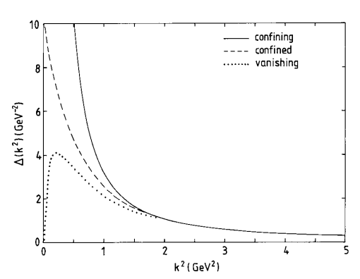
Figure 1: Possible behaviour of the gluon propagator $\Delta(k^{2})$, which is the coefficient of the $g_{\mu\nu}$ or $\delta_{\mu\nu}$ component of $\Delta_{\mu\nu}(k)$.
(a) confining gluon, $\Delta\sim(k^{2})^{-2}$,
(b) confined gluon, $\Delta\sim(k^{2})^{-c}$ with $c$ very small,
(c) infrared vanishing gluon $\Delta\sim k^{2}$.
All are matched to the perturbative behaviour for $k$ larger than a few GeV.

2. Schwinger-Dyson equation for the gluon propagator

The Schwinger-Dyson equations are coupled integral equations which inter-relate the Green’s functions of a field theory. Since they build an infinite tower of coupled equations, approximations and truncations are necessary to solve them. The Schwinger-Dyson equation for the gluon propagator yields a relation for $\Delta_{\mu\nu}$ in terms of the full 3 and 4-point vertex functions, $\Gamma_{\mu\nu\rho}^{3}$ and $\Gamma_{\mu\nu\rho\sigma}^{4}$, the quark and the ghost propagators and couplings. The equation is displayed diagrammatically in Fig. 2. Here we only consider a pure gauge theory, i.e. a world without quarks. This is reasonable since we expect it is the non-Abelian nature of QCD which is responsible for confinement.

Figure 2: The Schwinger-Dyson equation for the gluon propagator
Here the broken line represents the ghost propagator. The symmetry factors 1/2 and 1/6 and a negative sign for every ghost and fermion loop arise from the usual Feynman rules.

3. Axial Gauge Studies

In the axial gauge the gluon propagator is transverse to the gauge vector $n_{\mu}$, so

Axial gauge formalism : $n_{\mu}A^{a\mu}=0$

Studies of the axial gauge Schwinger-Dyson equation have the advantage that ghost fields are absent and the four-gluon vertex terms, Fig. 2, may be projected out of the Schwinger-Dyson equation. However they have the drawback that the gluon propagator depends not only on $p^{2}$, but also on the unphysical gauge parameter $\gamma$, defined as

$$\gamma=\frac{(n\cdot p)^{2}}{n^{2}p^{2}}$$

and in general must depend on two scalar functions, $F$ and $H$ :

$$\Delta_{\mu\nu}(p^{2},\gamma)=-\frac{i}{p^{2}}\left[F(p^{2},\gamma)M_{\mu\nu}+H(p^{2},\gamma)N_{\mu\nu}\right]\quad,$$ (1)

with the tensors given by:

$$M_{\mu\nu}=g_{\mu\nu}-\frac{p_{\mu}n_{\nu}+p_{\nu}n_{\mu}}{n\cdot p}+n^{2}\frac{p_{\mu}p_{\nu}}{(n\cdot p)^{2}}\qquad,$$

$$N_{\mu\nu}=g_{\mu\nu}-\frac{n_{\mu}n_{\nu}}{n^{2}}\qquad.$$

The free propagator is obtained by substituting $F=1$ and $H=0$.

In all previous axial gauge studies it has been assumed that any infrared singular part of the propagator has the same tensor structure as the free one (though importantly this contradicts the results of West [13]). Thus for $p^{2}\rightarrow 0$ it is assumed that

$$\Delta_{\mu\nu}(p^{2},\gamma)=-\frac{i}{p^{2}}\,F(p^{2},\gamma)M_{\mu\nu}\qquad.$$ (2)

The gluon vacuum polarization tensor $\Pi_{\lambda\mu}(p^{2},\gamma)$ is defined by

$$\Pi^{\lambda\mu}\ \Delta_{\mu\nu}=g^{\lambda}_{\ \nu}-\frac{n^{\lambda}p_{\nu}}{n\cdot p}\qquad.$$

Projecting the integral equation with ${n_{\mu}n_{\nu}}/{n^{2}}$ the loops involving the four gluon vertex give an identically zero contribution because of the tensor structure of the bare 4-gluon vertex and the fact that the gluon propagator is transverse to the axial gauge vector, that is

$$n_{\mu}\Delta^{\mu\nu}=0=\Delta^{\mu\nu}n_{\nu}\qquad.$$

Thus the relevant part of the Schwinger-Dyson equation of Fig. 2 becomes:

$$\Pi_{\mu\nu}=\Pi_{\mu\nu}^{(0)} - \frac{g^{2}}{2}\int\frac{d^{4}k}{(2\pi)^{4}}\ \Gamma_{\mu\alpha\delta}^{(0)}(-p,k,q)\ \Delta^{\alpha\beta}(k)\ \Delta^{\gamma\delta}(q)\ \Gamma_{\beta\gamma\nu}(-k,p,-q)\$$ (3)

$$- \frac{g^{2}}{2}\int\frac{d^{4}k}{(2\pi)^{4}}\ \Gamma_{\mu\nu\alpha\beta}^{0}(p,k,-k,-p)\ \Delta^{\alpha\beta}(k)$$

where $q=p-k$, the last term is the tadpole contribution and all colour indices are implicitly included in the vertices. Once the full 3-gluon vertex is known, we have a closed equation for the gluon vacuum polarization $\Pi_{\mu\nu}$.

The vertex is constrained by the Slavnov-Taylor identity in terms of this vacuum polarization :

$$q_{\nu}\Gamma^{\mu\nu\rho}(p,q,k)=\Pi^{\mu\rho}(k)-\Pi^{\mu\rho}(p)\qquad.$$ (4)

Separating $\Gamma^{\mu\nu\rho}$ into transverse and longitudinal part, where the transverse part is defined to vanish when contracted with any external momentum, the Slavnov-Taylor identity exactly determines the longitudinal part [12] if it is to be free of kinematic singularities. Thus

$$\Gamma_{\mu\nu\rho}^{L}(p,k,q) = g_{\mu\nu}\left(\frac{p_{\rho}}{F(p^{2},\gamma)}-\frac{q_{\rho}}{F(q^{2},\gamma)}\right)$$ (5)

$$+\frac{1}{p^{2}-q^{2}}\left(\frac{1}{F(p^{2},\gamma)}-\frac{1}{F(q^{2},\gamma)}\right)(p_{\nu}q_{\mu}-g_{\mu\nu}p\cdot q)(p_{\rho}-q_{\rho})$$

$$+\phantom{\frac{1}{p^{2}}}\ \mbox{cyclic permutations}\qquad.$$

This longitudinal part is responsible for the dominant ultraviolet structure of the vertex. Moreover, it is assumed, that it entirely embodies the infrared behaviour, and so the transverse part can be neglected. This assumption is motivated by the fact that the transverse part (as defined) vanishes, when the external momenta approach zero.

Using the explicit expressions, Eq. (2) for $\Delta$, Eqs. (4,5) for $\Gamma$ and multiplying with ${n_{\mu}n_{\nu}}/{n^{2}}$, we find in Euclidean space:

$$-\frac{p^{2}}{F(p^{2})}\left(1-\gamma\right) = -p^{2}\left(1-\gamma\right)+\frac{g^{2}C_{A}}{2}\int\frac{d^{4}k}{(2\pi)^{4}}\frac{n\cdot(k-q)}{n^{2}}\Delta^{\lambda\rho}_{(0)}(k)\ \Delta^{\lambda\sigma}_{(0)}(q)$$ (6)

$$\left\{k\cdot n\left[\delta_{\rho\sigma}F(q^{2})-\frac{F(q^{2})-F(k^{2})}{k^{2}-q^{2}}(\delta_{\rho\sigma}k\cdot q-k_{\rho}q_{\sigma})\right.\right.$$

$$\qquad\qquad\qquad\left.+\frac{F(k^{2})-F(p^{2})}{p^{2}-k^{2}}\frac{F(q^{2})}{F(p^{2})}p_{\sigma}(p+k)_{\rho}\right]$$

$$-q\cdot n\ \left[\delta_{\rho\sigma}F(k^{2})-\frac{F(q^{2})-F(k^{2})}{k^{2}-q^{2}}(\delta_{\rho\sigma}k\cdot q-k_{\rho}q_{\sigma})\right.$$

$$\qquad\qquad\qquad\left.\left.+\frac{F(q^{2})-F(p^{2})}{p^{2}-q^{2}}\frac{F(k^{2})}{F(p^{2})}p_{\rho}(q+p)_{\sigma}\right]\right\}$$

$$+\frac{g^{2}C_{A}}{2}\int\frac{d^{4}k}{(2\pi)^{4}}\frac{F(k^{2})}{k^{2}}\left(2+\frac{k^{2}n^{2}}{(n\cdot k)^{2}}\right)\qquad.$$

This is the equation first found by Baker, Ball and Zachariasen [4] who studied its solution numerically. They came to the conclusion that the only consistent infrared behaviour for the function $F(p^{2})$ is

$$F(p^{2})\propto\frac{1}{p^{2}}\ \ \ \mbox{as}\ p^{2}\ \rightarrow 0$$

and that this is independent of $\gamma$ as a numerical approximation.

Schoenmaker [6] simplified the BBZ equation further by exactly setting $\gamma=0$. Doing this the contribution of the tadpole diagram vanishes. Moreover, approximating $F(q^{2})$ by $F(p^{2}+k^{2})$, which should be exact in the infrared limit, allows the angular integrals to be performed analytically. Consequently, Schoenmaker finds the following simpler equation:

$$p^{2}\left(\frac{1}{F(p^{2})}-1\right)=$$ (7)

$$\frac{g^{2}C_{A}}{32\pi^{2}}\left\{\int_{0}^{p^{2}}dk^{2}\left[\left(-\frac{k^{4}}{12p^{4}}+\frac{5}{2}\frac{k^{2}}{p^{2}}-\frac{2}{3}\frac{k^{2}}{p^{2}-k^{2}}\right)F_{1}+\left(\frac{k^{6}}{24p^{6}}-\frac{1}{4}\frac{k^{4}}{p^{4}}-\frac{1}{4}\frac{k^{2}}{p^{2}}\right)F_{2}\right.\right.$$

$$\qquad\quad\left.+\left(-\frac{1}{6}\frac{k^{2}}{p^{2}}+\frac{2}{3}\frac{k^{2}}{p^{2}-k^{2}}\right)F_{3}\right]+\int_{p^{2}}^{\infty}dk^{2}\left[\left(-\frac{3}{4}-\frac{p^{2}}{4k^{2}}-\frac{2}{3}\frac{p^{2}}{p^{2}-k^{2}}\right)F_{1}\right.$$

$$\qquad\quad\left.\left.+\left(-\frac{3}{4}\frac{k^{2}}{p^{2}}+\frac{5}{12}-\frac{1}{8}\frac{p^{2}}{k^{2}}\right)F_{2}+\left(\frac{7}{6}\frac{p^{2}}{k^{2}}+\frac{2}{3}\frac{p^{2}}{p^{2}-k^{2}}\right)F_{3}\right]\right\}\qquad,$$

where

$$F_{1} = F(p^{2}+k^{2})\qquad\qquad,$$

$$F_{2} = F(p^{2}+k^{2})-F(k^{2})\quad,$$

$$F_{3} = \frac{F(p^{2}+k^{2})F(k^{2})}{F(p^{2})}\qquad.$$

In general, this equation has a quadratic ultraviolet divergence, which would give a mass to the gluon. Such terms have to be subtracted to ensure the masslessness condition

$$\lim_{p^{2}\rightarrow 0}\Pi_{\mu\nu}=0\ \ \mbox{, i.e.}\ \ \ \frac{p^{2}}{F(p^{2})}=0\ \ \mbox{for}\ \ p^{2}\rightarrow 0\qquad,$$ (8)

is satisfied. This property can be derived generally from the Slavnov-Taylor identity and always has to hold.

The complicated structure of the integral equation, Eq. (7), does not allow an exact analytic solution for the gluon renormalization function $F(p^{2})$ to be found and most previous studies ([8], [10], [4] and [7]) solve the equation numerically. However, the possible asymptotic behaviour of $F(p^{2})$ for both small and large $p^{2}$ can be investigated analytically.

We determine which infrared behaviour of $F(p^{2})$ can give a self-consistent solution to the integral equation by taking a trial input function $F_{in}(p^{2})$ and substituting it into the right hand side of the equation. After performing the $k^{2}$-integration, we obtain an output function $1/F_{out}(p^{2})$ to be compared to the reciprocal of the input function. To do this, the gluon renormalization function is approximated in the infrared region by a Laurent expansion in powers of $p^{2}$ and at large momenta by its bare form, i.e.

$$F(p^{2})=\left\{\begin{array}[]{ll}\sum_{n=0}^{\infty}a_{n}\left(p^{2}/\mu^{2}\right)^{n+\eta}&\mbox{for \ $p^{2}<\mu^{2}$}\\ \\ 1&\mbox{for \ $p^{2}>\mu^{2}$}\end{array}\right.\qquad,$$ (9)

where

$$\sum_{n=0}^{\infty}a_{n}=1$$

to ensure continuity at $p^{2}=\mu^{2}$. $\mu$ is the mass scale above which we assume perturbation theory applies. $\eta$ can be negative to allow for an infrared enhancement. Eq. (9) is a sufficiently general representation for finding the dominant self-consistent infrared behaviour. Of course, the true renormalization function is modulated by powers of logarithms of momentum, characteristic of a gauge theory. However, these do not qualitatively affect the dominant infrared behaviour and can be neglected. Indeed to make the presentation straightforward, we only need approximate $F(p^{2})$ by its dominant infrared power $(p^{2})^{\eta}$ for $p^{2}<\mu^{2}$ to test whether consistency is possible and this is what we describe below. However, as we shall see, if $\eta$ is negative then potential mass terms arise and these have to be subtracted. Only in this case do higher terms in Eq. (9) play a role too and it is necessary to consider other than the leading term in the low momentum input. Otherwise higher powers make no qualitative difference as we have checked. Consequently we present only the results with the lowest powers in the representation, Eq. (9).

To illustrate the idea, let us take the trial infrared behaviour to be just

$$F(p^{2})\propto\left(\frac{p^{2}}{\mu^{2}}\right)^{\eta}\qquad\mbox{(i.e. $a_{n}=0$ for $n\geq 1$)}\qquad.$$ (10)

Note that the masslessness condition, Eq. (8), restricts $\eta$ to be less than 1. Furthermore we demand that in the high momentum region the solution of the integral equation matches the perturbative result, i.e. for $p^{2}\rightarrow\infty$, we have $F(p^{2})=1$, modulo logarithms.

Taking $\eta=-1$, for example, i.e.

$$F_{in}(p^{2})=A\frac{\mu^{2}}{p^{2}}$$

in Schoenmaker’s approximation, Eq. (7), gives

$$p^{2}\left(\frac{1}{F(p^{2})}-1\right)=\mbox{const}\qquad.$$

This violates the masslessness condition of Eq. (8) and so has to be mass renormalized. As explained above, now terms in $F(p^{2})$ of higher order in $p^{2}$ will generate a contribution to the right hand side of the equation making it possible to find a self-consistent solution by these cancelling the explicit factor of 1. Consequently, we can approximate Eq. (9) by

$$F_{in}(p^{2})=\left\{\begin{array}[]{ll}A\left({\mu^{2}}/{p^{2}}\right)+\left({p^{2}}/{\mu^{2}}\right)&\mbox{if $p^{2}<\mu^{2}$}\\ \\ 1&\mbox{if $p^{2}>\mu^{2}$}\end{array}\right.\qquad,$$ (11)

We then find, after mass renormalization:

$$\frac{1}{F_{out}(p^{2})}=1+\frac{g^{2}C_{A}}{32\pi^{2}}\left[\frac{67}{96}\frac{p^{2}}{\mu^{2}}-\frac{1}{12}-\frac{3}{8}\frac{p^{2}}{\mu^{2}}\ln\left(\frac{\mu^{2}}{p^{2}}\right)+\frac{5}{12}\ln\left(\frac{\Lambda^{2}}{\mu^{2}}\right)\right]\qquad,$$ (12)

where $\Lambda$ is the ultraviolet cut-off introduced to make the integrals finite. The ultraviolet divergent constant can be arranged to cancel the 1 and we find self-consistency modulo logarithms. It is this result that Schoenmaker found [6] supporting the earlier result of BBZ [4]. However, importantly, self-consistency requires $A$, Eq. (11), to be negative as also found by Schoenmaker.

More recently, Cudell and Ross [7] have taken Schoenmaker’s equation, Eq. (7), and investigated whether one can find self-consistency for a gluon renormalization function which is less singular than $1/k^{2}$ for $k^{2}\rightarrow 0$, i.e. which corresponds to confined gluons. The trial input function they use in their investigation is

$$F_{in}(p^{2})\propto(p^{2})^{1-c}\qquad,$$

where c is small and positive to ensure a massless gluon, Eq. (8). Once more we want the integral equation for $\Pi_{\mu\nu}$ to agree with perturbation theory in the ultraviolet region, but $F_{in}(p^{2})\propto(p^{2})^{1-c}$ grows for large momenta and hence spoils the ultraviolet behaviour. So to check whether this input function gives self-consistency in the infrared, we input the trial form :

$$F_{in}(p^{2})=\left\{\begin{array}[]{ll}\left({p^{2}}/{\mu^{2}}\right)^{1-c}&\mbox{if $p^{2}<\mu^{2}$}\\ \\ 1&\mbox{if $p^{2}>\mu^{2}$}\end{array}\right.\qquad.$$ (13)

Inserting this into Eq. (7), we find, after mass renormalization :

$$\frac{1}{F_{out}(p^{2})} = 1+\frac{g^{2}C_{A}}{32\pi^{2}}\left[\ D_{1}+\ D_{2}\left(\frac{\mu^{2}}{p^{2}}\right)^{1-c}+\ D_{3}\left(\frac{p^{2}}{\mu^{2}}\right)^{1-c}+\ D_{4}\left(\frac{p^{2}}{\mu^{2}}\right)^{c}+...\right],$$ (14)

where $F_{1},F_{2}$ and $F_{3}$ have been expanded for small $p^{2}$ and only the first few terms have been collected in this equation so that

$$D_{1} = \frac{5}{12(1-c)}-\frac{1}{3}+\frac{11}{12}\ln{\frac{\Lambda^{2}}{\mu^{2}}}\qquad,$$

$$D_{2} = \frac{1}{2(2-2c)}+\frac{1}{6}\ln\left(\frac{\Lambda^{2}}{\mu^{2}}\right)\qquad,$$

$$D_{3} = \frac{2407}{1440}-\frac{353c}{360}-\frac{3}{8c}-\frac{1}{24(5-c)}+\frac{1+2c}{12(4-c)}-\frac{7-8c}{12(3-c)}-\frac{7+c}{12(2-c)}-\frac{7}{12(1-c)}$$

$$+\frac{1-4c}{6(2-2c)}+\frac{3-7c}{6(1-2c)}+\frac{2}{3}(2-c)\Psi(1)-\frac{4}{3}(2-c)\Psi(1-c)+\frac{2}{3}(2-c)\Psi(1-2c)\ ,$$

$$D_{4} = -\frac{7-9c}{24c}\qquad,$$

where $\Psi$ is the logarithmic derivative of the Gamma function. Again the 1 can be arranged to cancel with the constant term and the dominant infrared behaviour is indeed

$$\frac{1}{F_{out}(p^{2})}\rightarrow\left(\frac{\mu^{2}}{p^{2}}\right)^{1-c}\ \ \ \ \mbox{for}\ \ p^{2}\rightarrow 0$$ (15)

Hence a gluon propagator less singular than $1/p^{2}$ for $p^{2}\rightarrow 0$ can be derived from Schoenmaker’s equation as Cudell and Ross [7] have found. Note once again that terms of higher order in Eq. (9) do not qualitatively alter the result. Thus we see in the axial gauges that apparently both confined and confining solutions are possible for the gluon propagator. However, the singular confining behaviour must be an artefact of the approximation that one of the gluon functions, $H$, vanishes, since West [13] has shown that in a gauge with only positive norm-states, a singular gluon renormalization function is not possible. Moreover, the approximation of setting $\gamma=0$ in the BBZ-equation, Eqs. (6,7), has been seriously questioned in Ref. [14]. It is therefore sensible to ask what is the behaviour in covariant gauges, to which we now turn.

4. Landau Gauge Studies

The advantage of Landau gauge studies is the much simpler structure of the gluon propagator, which is defined by :

$$\Delta_{\mu\nu}=-i\ \frac{G(p^{2})}{p^{2}}\left(g_{\mu\nu}-\frac{p_{\mu}p_{\nu}}{p^{2}}\right)\qquad.$$ (16)

However other problems arise and the following approximations have to be made :

• In any covariant gauge, ghosts are necessary to keep the vacuum polarization transverse and hence are present in the Schwinger-Dyson equation of the gluon propagator, Fig. 2. However, in all previous studies [8, 10] the ghost loop diagram is only included in as much as it ensures the transversality of the gluon propagator, assuming that otherwise it does not affect the infrared behaviour of the propagator. This assumption is supported by the fact, that in a one-loop perturbative calculation the ghost loop makes a numerically small contribution to $G(p^{2})$.

• The 4-gluon terms cannot be eliminated as in the axial gauge and are simply neglected. This can be regarded as a first step in a truncation of the Schwinger-Dyson equations.
  

With these assumptions, we again find a closed integral equation for the gluon vacuum polarization, $\Pi_{\mu\nu}$, once the full 3-gluon vertex is known. In the Landau gauge, the Slavnov-Taylor identity for the 3-gluon vertex involves the ghost self-energy, which is simply set to zero, and the proper ghost-gluon vertex function $G_{\mu\nu}$. However, in the limit of vanishing ghost momentum the ghost-gluon vertex is approximately equal to the gluon propagator. With this simplification the Slavnov-Taylor identity has the same form as in the axial gauge and is given in Eq. (5). Once again neglecting the transverse part of the vertex, we obtain a closed integral equation :

$$\Pi_{\mu\nu}=\Pi_{\mu\nu}^{(0)}-\frac{g^{2}}{2}\ \int\frac{d^{4}k}{(2\pi)^{4}}\ \Gamma_{\mu\alpha\delta}^{(0)}(-p,k,q)\ \Delta^{\alpha\beta}(k)\ \Delta^{\gamma\delta}(q)\ \Gamma_{\beta\gamma\nu}(-k,p,-q)$$ (17)

where once again the colour indices are implicit and $q=p-k$.

A scalar equation is obtained by projecting with

$$P^{\mu\nu}=\frac{1}{3p^{2}}(4p^{\mu}p^{\nu}-p^{2}g^{\mu\nu})$$

This projector has the advantage that the $g_{\mu\nu}$ term in Eq. (16) that is quadratically divergent in 4-dimensions, does not contribute. Thus we find

$$\frac{1}{G(p^{2})}=1+\frac{g^{2}C_{A}}{96\pi^{4}}\frac{1}{p^{2}}\int d^{4}k\left[G(q^{2})A(k^{2},p^{2})+\frac{G(k^{2})G(q^{2})}{G(p^{2})}\ B(k^{2},p^{2})\right.$$ (18)

$$\qquad\quad+\left.\frac{G(k^{2})-G(p^{2})}{k^{2}-p^{2}}\frac{G(q^{2})}{G(p^{2})}\ C(k^{2},p^{2})+\frac{G(q^{2})-G(k^{2})}{q^{2}-k^{2}}\ D(k^{2},p^{2})\right],$$

where

$$A(k^{2},p^{2}) = 48\frac{(k\cdot p)^{2}}{k^{2}p^{2}q^{2}}-64\frac{(k\cdot p)}{k^{2}q^{2}}+16\frac{(k\cdot p)^{3}}{k^{2}p^{2}q^{4}}-12\frac{1}{k^{2}}+22\frac{p^{2}}{k^{2}q^{2}}-42\frac{(k\cdot p)^{2}}{k^{2}q^{4}}-10\frac{p^{4}}{k^{2}q^{4}}$$

$$+36\frac{p^{2}(k\cdot p)}{k^{2}q^{4}}\qquad,$$

$$B(k^{2},p^{2}) = -13\frac{p^{2}}{q^{4}}+18\frac{p^{2}(k\cdot p)}{k^{2}q^{4}}-2\frac{(k\cdot p)^{2}}{k^{2}q^{4}}-4\frac{p^{4}}{k^{2}q^{4}}+\frac{p^{2}(k\cdot p)^{2}}{k^{4}q^{4}}\;,$$

$$C(k^{2},p^{2}) = 4\frac{(k\cdot p)^{2}}{k^{2}q^{2}}+6\frac{p^{2}(k\cdot p)}{k^{2}q^{2}}+6\frac{(k\cdot p)}{q^{2}}+8\frac{p^{2}}{q^{2}}\quad,$$

$$D(k^{2},p^{2}) = 12\frac{k^{2}}{q^{2}}-48\frac{(k\cdot p)^{2}}{p^{2}q^{2}}+48\frac{(k\cdot p)^{3}}{k^{2}p^{2}q^{2}}+24\frac{(k\cdot p)}{q^{2}}-5\frac{p^{2}}{q^{2}}-40\frac{(k\cdot p)^{2}}{k^{2}q^{2}}+9\frac{p^{2}(k\cdot p)}{k^{2}q^{2}}\,.$$

Brown and Pennington [10] studied this equation numerically and found

$$G(p^{2})=A\,\frac{\mu^{2}}{p^{2}}\ \ \ \ \mbox{for}\ \ p^{2}\rightarrow 0$$

to be a consistent solution. This result is in agreement with Mandelstam’s study of the gluon propagator [8].

Again approximating $G(q^{2})$ by $G(p^{2}+k^{2})$ allows us to perform the angular integrals analytically in Eq. (18), giving:

$$\frac{1}{G(p^{2})}=1+$$ (19)

$$\frac{g^{2}C_{A}}{48\pi^{2}}\frac{1}{p^{2}}\left\{\int_{0}^{p^{2}}dk^{2}\left[G_{1}\left(-1-10\frac{k^{2}}{p^{2}}+6\frac{k^{4}}{p^{4}}+\frac{k^{2}}{p^{2}-k^{2}}\left(\frac{75}{4}-\frac{39}{4}\frac{k^{2}}{p^{2}}+4\frac{k^{4}}{p^{4}}-5\frac{p^{2}}{k^{2}}\right)\right)\right.\right.$$

$$\left.\qquad\qquad+G_{2}\left(-\frac{21}{4}\frac{k^{2}}{p^{2}}+7\frac{k^{4}}{p^{4}}-3\frac{k^{6}}{p^{6}}\right)+G_{3}\left(\frac{k^{2}}{p^{2}-k^{2}}\left(-\frac{27}{8}-\frac{11}{4}\frac{k^{2}}{p^{2}}-\frac{15}{8}\frac{p^{2}}{k^{2}}\right)\right)\right]$$

$$\qquad\qquad+\int_{p^{2}}^{\infty}dk^{2}\left[G_{1}\left(\frac{p^{2}}{k^{2}}-6+\frac{p^{2}}{p^{2}-k^{2}}\left(\frac{29}{4}+\frac{3}{4}\frac{p^{2}}{k^{2}}\right)\right)\,+\right.$$

$$\qquad\qquad\left.\left.+G_{2}\left(-\frac{3}{2}+\frac{1}{4}\frac{p^{2}}{k^{2}}\right)+G_{3}\left(\frac{p^{2}}{p^{2}-k^{2}}\left(\frac{3}{4}-\frac{67}{8}\frac{p^{2}}{k^{2}}-\frac{3}{8}\frac{p^{4}}{k^{4}}\right)\right)\right]\right\}\,,$$

where

$$G_{1} = G(p^{2}+k^{2})\qquad\qquad,$$

$$G_{2} = G(p^{2}+k^{2})-G(k^{2})\quad,$$

$$G_{3} = \frac{G(k^{2})G(p^{2}+k^{2})}{G(p^{2})}\;.$$

Note that the integral equation has the usual ultraviolet divergences, but infrared divergences are also possible. The ultraviolet divergences can be handled in the standard way to give a renormalized function $G_{R}(p^{2})$ — this will not be discussed here. However we have to make the potentially infrared divergent integrals finite in order to calculate the integrals. The infrared regularization procedure proposed by Brown and Pennington [10] is to use the plus prescription of the theory of distributions, which is defined as follows:

$$\left(\frac{\mu^{2}}{k^{2}}\right)_{+}=\frac{\mu^{2}}{k^{2}}\ \ \ \ \ \mbox{for}\ \ \infty>k^{2}>0$$

and in the neighbourhood of $k^{2}=0$ it is a distribution that satisfies:

$$\int_{0}^{\infty}dk^{2}\left(\frac{\mu^{2}}{k^{2}}\right)_{+}S(k^{2},p^{2})=$$ (20)

$$\int_{0}^{p^{2}}dk^{2}\,\frac{\mu^{2}}{k^{2}}\left[S(k^{2},p^{2})-S(0,p^{2})\right]+\int_{p^{2}}^{\infty}dk^{2}\,\frac{\mu^{2}}{k^{2}}S(k^{2},p^{2})\;.$$

Simply taking

$$G_{in}(k^{2})=A\left(\frac{\mu^{2}}{k^{2}}\right)_{+}$$

as an input function once again leads to a mass term and higher terms in the expansion Eq. (8) are necessary. Then we do have the chance of finding self-consistency for a gluon propagator as singular as $1/k^{4}$ and hence confining quarks. With

$$G_{in}(p^{2})=\left\{\begin{array}[]{ll}A\left({\mu^{2}}/{p^{2}}\right)_{+}+\left({p^{2}}/{\mu^{2}}\right)&\mbox{if $p^{2}<\mu^{2}$}\\ \\ 1&\mbox{if $p^{2}>\mu^{2}$}\end{array}\right.\qquad,$$ (21)

we find, after mass renormalization:

$$\frac{1}{G_{out}(p^{2})}=1+\frac{g^{2}C_{A}}{48\pi^{2}}\left[-\frac{479}{24}\frac{p^{2}}{\mu^{2}}+\frac{13}{8}\frac{p^{2}}{\mu^{2}}\ln\left(\frac{\mu^{2}}{p^{2}}\right)-\frac{81}{4}-\frac{25}{4}\ln\left(\frac{\Lambda^{2}}{\mu^{2}}\right)\right]\qquad.$$ (22)

The ultraviolet divergent constant can be arranged to cancel the 1 and, again, we find self-consistency. This is the result found numerically by Brown and Pennington [10] with a positive infrared enhancement to the gluon renormalization function, i.e. $A>0$.

Now we check, whether it is possible in the Landau gauge, to find the behaviour Cudell and Ross discovered using Schoenmaker’s approximation in the axial gauge. With

$$G_{in}(p^{2})=\left\{\begin{array}[]{ll}\left({p^{2}}/{\mu^{2}}\right)^{1-c}&\mbox{if $p^{2}<\mu^{2}$}\\ \\ 1&\mbox{if $p^{2}>\mu^{2}$}\end{array}\right.$$ (23)

we find, again after mass renormalization:

$$\frac{1}{G_{out}(p^{2})} = 1+\frac{g^{2}C_{A}}{48\pi^{2}}\left[\ D_{1}+\ D_{2}\left(\frac{\mu^{2}}{p^{2}}\right)^{1-c}+\ D_{3}\left(\frac{p^{2}}{\mu^{2}}\right)^{1-c}+\ D_{4}\left(\frac{p^{2}}{\mu^{2}}\right)^{c}+...\right]\ ,$$ (24)

where

$$D_{1} = -\left(\frac{3}{2}+\frac{5+6c}{1-c}+\frac{25}{4}\ln\left(\frac{\Lambda^{2}}{\mu^{2}}\right)\right)\qquad,$$

$$D_{2} = -\left(\frac{3}{4(2-2c)}+\frac{3}{4}\ln\left(\frac{\Lambda^{2}}{\mu^{2}}\right)\right)\qquad,$$

$$D_{3} = -\frac{1971}{60}+\frac{29c}{2}+\frac{37}{20c}+\frac{6-13c}{2(1-c)}+\frac{59-32c}{4(2-c)}+\frac{155-64c}{8(3-c)}$$

$$+\frac{127-49c}{8(4-c)}+\frac{23-11c}{4(5-c)}-\frac{125+61c}{8(1-2c)}-\frac{55+6c}{8(2-2c)}+\frac{3}{4(3-2c)}$$

$$-8(2-c)\Psi(-2c)-8(2-c)\Psi(1)\phantom{\frac{2}{2}}\qquad,$$

$$D_{4} = \frac{61+6c}{8(1-2c)}\qquad.$$

Thus the dominant infrared behaviour is:

$$\frac{1}{G_{out}(p^{2})}\rightarrow-\left(\frac{\mu^{2}}{p^{2}}\right)^{1-c}$$

and self-consistency is spoiled by a negative sign, since $c$ is small and positive.

5. Confined Gluons

A gluon propagator, which is less singular than $1/k^{2}$ for $k^{2}\rightarrow 0$, and hence describes confined gluons appears to be a self-consistent solution only of the axial gauge Schwinger-Dyson equation using Schoenmaker’s approximate integral Eq. (7). In the Landau gauge this behaviour of the gluon propagator is not possible : a minus-sign spoils self-consistency. We should therefore comment on the origin of this crucial minus sign.

Starting from BBZ’s integral Eq. (6), there is no difference in sign between the two gauges. Eq. (6) is Bose-symmetric (as it should be) and can therefore be rewritten as :

$$\frac{p^{2}}{F(p^{2})}\left(1-\gamma\right)=p^{2}\left(1-\gamma\right)$$ (25)

$$-\frac{g^{2}C_{A}}{2}\,\int\frac{d^{4}k}{(2\pi)^{4}}\frac{n\cdot(k-q)}{n^{2}}\,\Delta^{\lambda\rho}_{(0)}(k)\Delta^{\lambda\sigma}_{(0)}(q)\,2k\cdot n\ K_{\rho\sigma}(k,p)$$

where

$$K_{\rho\sigma}(k,p)= \delta_{\rho\sigma}F(q^{2})-\frac{F(q^{2})-F(k^{2})}{k^{2}-q^{2}}(\delta_{\rho\sigma}k\cdot q-k_{\rho}q_{\sigma})$$

$$+ \frac{F(k^{2})-F(p^{2})}{p^{2}-k^{2}}\frac{F(q^{2})}{F(p^{2})}\ (p+k)_{\rho}p_{\sigma}$$

whereas, taking the starting equation of Schoenmaker’s paper (Eq 3.5 of Ref. [6]) we find:

$$\frac{p^{2}}{F(p^{2})}\left(1-\gamma\right)=p^{2}\left(1-\gamma\right)$$ (26)

$$-\frac{i}{2}g^{2}C_{A}\int\frac{d^{4}k}{(2\pi)^{4}}\,\frac{n\cdot(k-q)}{n^{2}}\,\Sigma_{\rho\sigma}(k,q)[-2k\cdot n\ K_{\rho\sigma}(k,p)]$$

where

$$\Sigma_{\rho\sigma}(k,q)=(i)^{2}\Delta^{\lambda\rho}_{(0)}(k)\Delta^{\lambda\sigma}_{(0)}(q)\qquad.$$

Schoenmaker formulates his equation in Minkowski space. Performing a Wick rotation to transform to Euclidean space by : $d^{4}k_{M}\rightarrow id^{4}k_{E}$, we find that Schoenmaker’s equation, Eq. (26), becomes :

$$\frac{p^{2}}{F(p^{2})}\left(1-\gamma\right)=p^{2}\left(1-\gamma\right)$$ (27)

$$+\frac{g^{2}C_{A}}{2}\,\int\frac{d^{4}k}{(2\pi)^{4}}\frac{n\cdot(k-q)}{n^{2}}\,\Delta^{\lambda\sigma}_{(0)}(k)\Delta^{\lambda\rho}_{(0)}(q)\,2k\cdot n\ K_{\sigma\rho}(k,p)$$

which differs from Eq. (25) by a crucial minus sign.

We therefore see that in the axial gauge using BBZ’s integral equation for the gluon propagator, and simplifying the angular dependence in the way Schoenmaker does in order to make an analytical discussion of the infrared behaviour of the propagator possible, yields an integral equation very similar to the one found by Brown and Pennington [10] in the Landau gauge. These equations lead to the correct perturbative behaviour at large momenta. In contrast a self-consistent solution of the gluon propagator less singular than $1/k^{2}$ for $k^{2}\rightarrow 0$ cannot be found in either gauge. Schoenmaker’s own equation, which is the starting point for the study of Cudell and Ross [7] for instance, has an incorrect additional minus sign. This should have been heralded by the self-consistent enhanced gluon of Eq. (11) having a negative sign, using Schoenmaker’s equation. In an axial gauge this sign should have been a little worrying for a wavefunction renormalization of a state with positive definite norm.

6. Summary and Conclusion

We have studied the Schwinger-Dyson equation of the gluon propagator to determine analytically the possible infrared solutions for the gluon renormalization function $G(p^{2})$. In both the axial and Landau gauges, one can find a self-consistent solution, which behaves as $1/k^{2}$ for $k^{2}\rightarrow 0$ and hence a propagator which is as singular as $1/k^{4}$ for $k^{2}\rightarrow 0$. This form of the gluon propagator is consistent with area law behaviour of the Wilson loop, which is regarded as a signal for confinement . Numerical studies [4], [10] have shown that a gluon propagator with such an enhanced behaviour in the infrared region that connects to the perturbative regime at a finite momentum (as indicated by experiment) can indeed be found as a self-consistent solution to the boson Schwinger-Dyson equation. Such a behaviour of the boson propagator has been shown to give quark propagators with no physical poles [18]. Furthermore, extending these non-perturbative methods to hadron physics, it has been found that a regularized, infrared singular gluon propagator together with the Schwinger-Dyson equation for the quark self-energy, gives rise to a good description of dynamical chiral symmetry breaking. For instance, one obtains values for quantities such as the pion decay constant that agree with experimental results [11].

A gluon propagator which is less singular than $1/k^{2}$ for $k^{2}\rightarrow 0$, and hence describes confined gluons, cannot be found in either the axial or the Landau gauge. Solutions of this type have only been found using approximations to the gluon Schwinger-Dyson equation with an incorrect sign. Possible consequences for models of the pomeron are discussed elsewhere [19].

We should also mention the related work of the group of Stingl et al. [15]. They too start from an approximate, but larger, set of Schwinger-Dyson equations, which is then to be solved self-consistently. However, the method employed is completely different. The philosophy [15] is to obtain the solution of these equations as power series in the coupling, as in perturbation theory, and to include non-perturbative effects by letting each Green’s function depend upon a spontaneously generated mass scale, $b(g^{2})$. The gluon propagator is assumed to be of the form (see Fig. 1)

$$\Delta(k^{2})\equiv\frac{G(k^{2})}{k^{2}}=\frac{k^{2}}{k^{4}+b^{4}}\qquad,$$ (28)

representing confined gluons. This grossly violates the masslessness condition of Eq. (8). In general, gluon masses can only arise in 4-dimensions if the vertex functions have singularities themselves corresponding to coloured massless scalar states, otherwise the Slavnov-Taylor identities sufficiently constrain the vertex functions to require the inverse of the gluon propagator to vanish at $k\rightarrow 0$ . Not only do the vertices of Stingl et al. have these massless singularities but self-consistency can only be found if the 3-gluon vertex is complex, when conventional understanding of its singularity structure would lead us to expect it to be real for momenta which in Minkowski space are spacelike. Subsequently Hawes, Roberts and Williams [16] and Alkofer and Bender [17] have shown that with this gluon propagator, Eq. (28), the solution of the quark Schwinger-Dyson equation does not describe a confined particle. They therefore also conclude that the full gluon propagator in QCD cannot vanish in the infrared region.

To summarise:

At first sight there appears to be a distinction between a confining and a confined gluon. A confining gluon is one whose interactions lead to quark confinement. $\Delta(k^{2})\sim 1/k^{4}$ behaviour is of this confining type. In contrast, it is sometimes argued that $\Delta(k^{2})$ must be less singular than $1/k^{2}$ to ensure that gluons themselves do not propagate over large distances. However, whether gluons are confining or confined are not real alternatives. Gluons must be both. They confine quarks by having very strong long range interactions. They themselves are confined by not having a Lehman representation that any physical asymptotic state must have [11].

While infrared singular gluons satisfy both criteria, softened gluons though confined, do not generate quark confinement or dynamical chiral symmetry breaking, which are features of our world. Remarkably, a study of the field equations of QCD reveals this theory naturally exhibits these aspects with an infrared enhanced gluon propagator.

Acknowledgements

KB thanks the University of Durham for the award of a research studentship. We are grateful to Douglas Ross for repeating our calculations and confirming that the sign in Schoenmaker’s Eq. (3.5) is incorrect. Many of the underlying ideas discussed here were formulated by MRP in collaboration with Nick Brown — his memory lingers on.

References

• [1] G.B. West, Phys. Lett. B115, 468 (1982).
• [2] C.D. Roberts, A.G. Williams and G. Krein, Int. J. Mod. Phys.
A7, 5607 (1992).
• [3] P.V. Landshoff and O. Nachtmann, Z. Phys. C39, 405 (1989).
• [4] M. Baker, J.S. Ball and F. Zachariasen, Nucl. Phys. B186, 531 (1981),
ibid. B186, 560 (1981).
• [5] A.I. Alekseev, Yad. Fiz. 33, 516 (1981) [Sov. J. Nucl. Phys. 33, 269 (1981)];
F. Paccanoni, Nuovo Cim. A74, 267 (1983).
• [6] W.J. Schoenmaker, Nucl. Phys. B194, 535 (1982).
• [7] J.R. Cudell and D.A. Ross, Nucl. Phys. B359, 247 (1991).
• [8] S. Mandelstam, Phys. Rev. D20, 3223 (1979).
• [9] U. Bar-Gadda, Nucl. Phys. B163, 312 (1980).
• [10] N. Brown and M.R. Pennington, Phys. Lett. B202, 257 (1988), Phys. Rev.
D39, 2723 (1989).
• [11] C.D. Roberts and A.G. Williams,
β€œDyson-Schwinger Equations and their Application to Hadronic Physics”,
Progress in Particle and Nuclear Physics 33, 477 (1994).
• [12] J.S. Ball and T.W. Chiu, Phys. Rev. D22, 2550 (1980).
• [13] G.B. West, Phys. Rev. D27, 1878 (1983).
• [14] D. Atkinson, P.W. Johnson, W.J. Schoenmaker and H.A. Slim , Nuovo Cim.
A77, 197 (1983);
E.L. Heck and H.A. Slim, Nuovo Cim. A88, 407 (1985).
• [15] U.HΓ€bel, R. KΓΆnning, H.G. Reusch, M. Stingl and S. Wigard, Z. Phys.
A336, 435 (1990).
• [16] F.T. Hawes, C.D. Roberts and A.G. Williams, Phys. Rev. D49, 4683 (1994).
• [17] R. Alkofer and A. Bender, UniversitΓ€t TΓΌbingen preprint UNITU-THEP-15/1994.
• [18] For example: R.L. Stuller, Phys. Rev. D13, 513 (1976);
H. Pagels, Phys. Rev. D15, 2991 (1977).
• [19] K. BΓΌttner and M.R. Pennington, Univ. of Durham preprint DTP-95/54 (June 1995)
• [20] D. Zwanziger, Nucl. Phys. B364, 127 (1991).
• [21] J.E. Mandula and M. Ogilvie, Nucl. Phys. B1A (Proc.Suppl.) 117 (1987),
Phys. Lett. B185, 127 (1987);
C. Bernard, C. Parrinello and A. Soni, Phys. Rev. D49, 1585 (1994).