The Nonresonant Cabibbo Suppressed Decay $B^{\pm}\rightarrow\pi^{+}\pi^{-}\pi^{\pm}$
and Signal for CP Violation

Abstract

We consider various contributions to the nonresonant decay $B^{\pm}\rightarrow\pi^{+}\pi^{-}\pi^{\pm}$, both of the long-distance and short-distance types with the former providing for most of the branching ratio, predicted to be $BR(B^{\pm}\rightarrow\pi^{+}\pi^{-}\pi^{\pm})=(1.5-8.4)\times 10^{-5}$. We also discuss an application to CP violation resulting from the interference of that nonresonant background (with $m(\pi^{+}\pi^{-})\approx 3.4$ GeV) and $B^{\pm}\rightarrow\chi_{c0}\pi^{\pm}$ followed by $\chi_{c0}\rightarrow\pi^{+}\pi^{-}$. The resulting value of the partial rate asymmetry is $(0.40\sim 0.48)\mbox{sin}\gamma$, where $\gamma=\mbox{arg}(V_{ub}^{*})$.

Two body and quasi two body non-leptonic decays of heavy mesons have been extensively studied[1]. Multibody non-leptonic decays are more difficult to estimate, and one usually resorts to statistical or phase space models[2]. In this letter we will not discuss, for reasons that will become clear, heavy meson decays through a chain of real resonances[3], i.e. we consider only the nonresonant background, and confine ourselves to $B^{\pm}\rightarrow\pi^{+}\pi^{-}\pi^{\pm}$ though similar results are expected for $B\rightarrow KK\pi$ and other modes. Our motivation is two-fold:

1. $B^{\pm}\rightarrow\pi^{+}\pi^{-}\pi^{\pm}$ is expected to be larger than $B\rightarrow\pi\pi$, which though not separated yet experimentally from $B\rightarrow K\pi$, is estimated to have a branching ratio of the order $10^{-5}$[4]. It is therefore challenging to find a viable dynamical description of $B\rightarrow\pi\pi\pi$.

2. Recently[5],it has been suggested that large CP asymmetries should occur in $B^{\pm}\rightarrow h\pi^{\pm}$ where the hadronic state $h=\pi^{+}\pi^{-}$ has energy corresponding to the resonance $\chi_{c0}(3.4)$.

The absorptive phase necessary to observe CP violation in partial rate asymmetries, is provided by the $\chi_{c0}$ width (subtracting the small partial width of $\chi_{c0}$ to $\pi^{+}\pi^{-}$). The CP odd phase $\gamma$ results from the interference of the two quark processes responsible for the background decay $B\rightarrow\pi\pi\pi$ and $B\rightarrow\chi_{c0}\pi$, which are $b\rightarrow u\bar{u}d$ and $b\rightarrow c\bar{c}d$, respectively. The partial rate asymmetry obtained in Ref. [5] suffers from a large uncertainty due mostly to the unknown background and especially its angular dependence. Note that only $h=\pi^{+}\pi^{-}$ with spin-parity $0^{+}$ leads to interference with the resonant amplitude. Therefore, knowledge of the angular dependence is crucial, and this will come out directly once one has a reliable model for the background process $B\rightarrow\pi\pi\pi$. The interference between the resonance and the background amplitudes will then automatically project out the $0^{+}$ component of $h=\pi^{+}\pi^{-}$. Thus $\pi^{+}\pi^{-}$ arising from resonances like $\rho$ do not interfere and need not be considered.

In this letter we will consider three contributions to $B\rightarrow\pi\pi\pi$ and identify the leading one. As demonstrated below, the branching ratio for the background process will suffer from a large uncertainty, but the CP violating partial rate asymmetry will be affected only mildly by this uncertainty.

Let us now consider the three possible contributions to the nonresonant background $B\rightarrow\pi\pi\pi$, as depicted in fig.1a-c. We choose our momenta as follows: $B^{-}(p_{B})\rightarrow\pi^{-}(p_{1})\pi^{+}(p_{2})\pi^{-}(p_{3})$ and always symmetrize by $p_{1}\leftrightarrow p_{3}$. Furthermore we define $s=(p_{B}-p_{1})^{2}=(p_{2}+p_{3})^{2}$ and $t=(p_{B}-p_{3})^{2}=(p_{1}+p_{2})^{2}$.

Diagram 1a is the short-distance contribution to $B\rightarrow\pi\pi\pi$, for which the effective weak Hamiltonian is

$$H_{eff}={G_{F}\over\sqrt{2}}V_{ub}V_{ud}^{*}(C_{1}O_{1}+C_{2}O_{2})\;,$$ (1)

where $C_{1}\approx-0.313$, $C_{2}\approx 1.15$, and

$$O_{1}=\bar{d}\gamma_{\mu}(1-\gamma_{5})b\bar{u}\gamma^{\mu}(1-\gamma_{5})u\;,\;\;O_{2}=\bar{u}\gamma_{\mu}(1-\gamma_{5})b\bar{d}\gamma^{\mu}(1-\gamma_{5})u\;.$$ (2)

Within the factorization approximation, we have the following amplitude

$$M_{a} = {G_{F}\over\sqrt{2}}V_{ub}V_{ud}^{*}<\pi^{+}\pi^{-}\pi^{-}|C_{1}O_{1}+C_{2}O_{2}|B^{-}>$$ (3)

$$= {G_{F}\over\sqrt{2}}V_{ub}V_{ud}^{*}(C_{1}+{C_{2}\over N_{c}})<\pi^{-}(p_{1})|\bar{d}\gamma_{\mu}b|B^{-}(p_{B})><\pi^{+}(p_{2})\pi^{-}(p_{3})|\bar{u}\gamma_{\mu}u|0>$$ (4)

$$+ (p_{1}\leftrightarrow p_{3})\;.$$ (5)

The matrix elements in Eq.(3), neglecting $m_{\pi}^{2}$ are

$$<\pi^{-}|\bar{d}\gamma_{\mu}b|B^{-}> = (p_{B}+p_{1})_{\mu}F^{B\pi}_{1}(s)+{m_{B}^{2}\over s}(p_{B}-p_{1})_{\mu}(F^{B\pi}_{0}(s)-F^{B\pi}_{1}(s))\;,$$ (6)

$$<\pi^{+}(p_{2})|\bar{u} \gamma_{\mu} u|\pi^{+}(-p_{3})>=(p_{2}-p_{3})_{\mu}F_{1}^{\pi\pi}(s)\;.$$ (7)

Substituting in Eq.(3) and performing the scalar products lead to

$$M_{a}={G_{F}\over\sqrt{2}}|V_{ub}V_{ud}^{*}|e^{-i\gamma}a_{2}[F^{B\pi}_{1}(s)F^{\pi\pi}_{1}(s)(2t+s-m_{B}^{2})+F^{B\pi}_{1}(t)F^{\pi\pi}_{1}(t)(2s+t-m_{B}^{2})]\;.$$ (8)

We have defined $a_{2}=C_{1}+C_{2}/N_{c}$, but will take the phenomenological value $a_{2}\approx 0.24$[6], and $\gamma=\mbox{arg}(V_{ub}^{*})$. For the form factors above we use pole model forms[7]

$$F_{1,0}^{B\pi}(q^{2})={F^{B\pi}_{1,0}(0)\over 1-q^{2}/m_{1,0}^{2}}\;,\;\;F^{\pi\pi}_{1}(q^{2})={1\over 1-q^{2}/m_{\pi\pi}^{2}+i\Gamma_{\sigma}/m_{\pi\pi}}\;,$$ (9)

where $F_{1}^{B\pi}(0)=F^{B\pi}_{0}(0)=0.333$[8], or $0.53\pm 0.12$[9] and $m_{1}=5.32$ GeV, $m_{0}=5.78$ GeV, $m_{\pi\pi}\approx m_{\sigma}=0.7$ GeV and $\Gamma_{\sigma}=0.2$ GeV.

Substituting the appropriate numerical values, integrating over phase space and using [10] $\tau_{B}=1.54\times 10^{-12}$ s, we find that the contribution of diagram 1a to the branching ratio is

$$BR_{a}={\Gamma_{a}\over\Gamma_{B}}=0.9\times 10^{-6}\left({F^{B\pi}_{1}(0)\over 0.333}\right)^{2}$$ (10)

which ranges between $0.9\times 10^{-6}$ and $2.3\times 10^{-6}$.

Diagram 1b which is obviously of the long-distance type is harder to calculate than diagram 1a. It is nevertheless small as the intermediate pion is highly off-shell. The weak transition $B\rightarrow\pi$ is easy to evaluate, and leads to

$$T(B\rightarrow\pi) = <\pi^{-}|{G_{F}\over\sqrt{2}}V_{ub}V_{ud}^{*}(C_{1}O_{1}+C_{2}O_{2})|B^{-}>$$ (11)

$$= {G_{F}\over\sqrt{2}}V_{ub}V_{ud}^{*}a_{1}f_{B}f_{\pi}m_{B}^{2}\;,$$ (12)

where $a_{1}=C_{1}/N_{c}+C_{2}\approx 1.1$, $f_{B}=0.2$ GeV and $f_{\pi}=0.13$ GeV. Then, again neglecting $m_{\pi}$, we find

$$M_{b}={G_{F}\over\sqrt{2}}V_{ub}V_{ud}^{*}a_{1}f_{B}f_{\pi}A(\pi\pi\pi\pi)\;.$$ (13)

$A(\pi\pi\pi\pi)$ is not known for one highly off-shell pion and three on-shell ones. If we assume only S-wave, and use the unitarity limit, $A(\pi\pi\pi\pi)\sim O(1)$, the branching ratio contribution of $M_{b}$ is

$$BR_{b}={\Gamma_{b}\over\Gamma_{B}}<10^{-8}\;.$$ (14)

Of course it is unrealistic to assume only S-wave contribution to $M_{b}$, and waves with angular momenta up to $ka$ contribute, where $k$ is the momentum in the center of mass and $a$ is a typical size. It is difficult to make our estimates more quantitative since one of the pions is highly off-shell. However we can not to envision this contribution to be large, and we shall neglect it.

Turning to diagram 1c, which is also of a long-distance type, we will show that it is the dominant diagram and its branching ratio is equal or larger than $BR(B\rightarrow\pi\pi)$ which should clearly be the case, since even in the charmed meson system[10] $\Gamma(D\rightarrow\pi\pi\pi)\geq\Gamma(D\rightarrow\pi\pi)$. The calculation of the amplitude $M_{c}$ involves the application of both Heavy Quark Effective Theory (HQET) and Chiral Perturbation Theory (CHPT). For a review of both see Ref.[11]. First we write

$$M_{c}=A^{\mu}_{BB^{*}\pi}{-g_{\mu\nu}+p_{B^{*}\mu}p_{B^{*}\nu}/m^{2}_{B^{*}}\over p^{2}_{B^{*}}-m_{B^{*}}^{2}}A^{\nu}_{B^{*}\pi\pi}+(p_{1}\leftrightarrow p_{3})\;.$$ (15)

Note that the $B^{*}$ is off-shell and since we are interested in the nonresonant part of $B\rightarrow\pi\pi\pi$, no on-shell intermediate resonances are introduced. Our main aim now is to calculate the strong and weak vertices $A^{\mu}_{BB^{*}\pi}$ and $A^{\nu}_{B^{*}\pi\pi}$, respectively, using the methods of HQET and for the strong vertex combining them with CHPT[12].

Let us start by calculating $A^{\mu}_{BB^{*}\pi}$. The Heavy-Chiral Lagrangian density[11, 12] relevant to us is

$$\cal{L}\mbox{${}_{int}=ig\sqrt{m_{B}m_{B^{*}}}<H_{b}\gamma_{\mu}\gamma_{5}A^{\mu}_{ba}\bar{H}_{a}>$}\;,$$ (16)

where $<>$ stands for trace. The field $H_{a}$ describes the heavy-quark light-quark $(Q\bar{q}_{a})$ system and

$$H_{a} = {1+\not v\over 2}(P^{*}_{a\mu}\gamma^{\mu}-P_{a}\gamma_{5})\;,\;\;\bar{H}_{a}=\gamma_{0}H^{\dagger}\gamma_{0}\;,$$ (17)

$$A^{\mu}_{ba} = {1\over 2}(\xi^{\dagger}\partial^{\mu}\xi-\xi\partial^{\mu}\xi^{\dagger})_{ba}\;,$$ (18)

where $P_{a}=(B^{-},\bar{B}^{0}_{d},\bar{B}^{0}_{s})$ and similarly for $P^{*}_{a\mu}$ in terms of the vector meson states, $v$ is the heavy meson velocity, and $\xi=exp(iM/f_{\pi})$ with $M$ given by

$$M=\left(\begin{array}[]{ccc}{\pi^{0}\over\sqrt{2}}+{\eta\over\sqrt{6}}&\pi^{+}&K^{+}\\ \pi^{-}&-{\pi^{0}\over\sqrt{2}}+{\eta\over\sqrt{6}}&K^{0}\\ K^{-}&\bar{K}^{0}&-{2\eta\over\sqrt{6}}\end{array}\right)\;.$$ (22)

We obtain

$$A_{BB^{*}\pi}^{\mu}\epsilon_{\mu}=-{2g\over f_{\pi}}\sqrt{m_{B}m_{B^{*}}}B^{-}B^{*}_{\nu}\partial^{\nu}\pi^{+}\;.$$ (23)

Using the flavor symmetry of HQET the coupling constant $g$ is determined to be 0.6 from $D^{*}\rightarrow D\pi$ data[9, 12]. The main uncertainty in the application of Eq.(15) to our case is that in diagram 1c the $B^{*}$ is off-shell. We therefore define $\mu$ as a measure of the off-shellness of the $B^{*}$ and consider two cases: 1. $\mu=\sqrt{m_{B}m_{B^{*}}}$ in Eq.(15). 2. $\mu=\sqrt{m_{B}\sqrt{p_{B^{*}}^{2}}}$, where $p_{B^{*}}$ is the momentum of the $B^{*}$.

To calculate $A_{B^{*}\pi\pi}$ in Eq.(11), we employ the spin independence of HQET and write

$$A_{B^{*}\pi\pi}^{\nu}\epsilon_{\nu} = {G_{F}\over\sqrt{2}}V_{ub}V_{ud}^{*}<\pi^{+}\pi^{-}|C_{1}O_{1}+C_{2}O_{2}|B^{*}>$$ (24)

$$= {G_{F}\over\sqrt{2}}V_{ub}V_{ud}^{*}a_{1}<\pi^{+}|\bar{u}\gamma_{\mu}(1-\gamma_{5})b|B^{*}><\pi^{-}|\bar{d}\gamma^{\mu}(1-\gamma)u|0>\;.$$ (25)

The form factors $T_{1-4}$ are defined as follows

$$<\pi^{+}|\bar{u}\gamma_{\mu}b|B^{*}> = 2T_{1}i\epsilon_{\mu\nu\lambda\sigma}\epsilon^{\nu}p^{\lambda}_{B^{*}}p^{\sigma}_{2}\;,$$ (26)

$$<\pi^{+}|\bar{u}\gamma_{\mu}\gamma_{5}b|B^{*}> = 2T_{2}m_{B^{*}}^{2}\epsilon_{\mu}+2T_{3}(\epsilon\cdot q)(p_{B^{*}}+p_{2})_{\mu}+2T_{4}(\epsilon\cdot q)(p_{B^{*}}-p_{2})_{\mu}\;,$$ (27)

where $q=p_{B^{*}}-p_{2}$. Relations between $T_{i}^{\prime}s$ and $f_{\pm}$ defined through

$$<\pi^{+} | \bar{u}\gamma_{\mu}b|\bar{B}^{0}>=f_{+}(p_{B}+p_{\pi})_{\mu}+f_{-}(p_{B}-p_{\pi})_{\mu}\;,$$ (28)

are

$$T_{1} = -i{f_{+}-f_{-}\over 2m_{B}}\;,\;\;T_{2}={1\over 2m_{B}^{2}}((f_{+}+f_{-})m_{B}+(f_{+}-f_{-}){p_{B}\cdot p_{\pi}\over m_{B}})\;,$$ (29)

$$T_{3} = {f_{+}-f_{-}\over 4m_{B}}\;,\;\;T_{4}=T_{3}\;.$$ (30)

Substituting the above relations in Eq.(16), we have

$$A_{B^{*}\pi\pi}^{\nu}\epsilon_{\nu}={G_{F}\over\sqrt{2}}V_{ub}V_{ud}^{*}a_{1}f_{\pi}(\epsilon\cdot p_{3})({3f_{+}\over 2}m_{B}+{f_{-}\over 2}m_{B}+(f_{+}-f_{-}){p_{2}\cdot p_{3}\over m_{B}})\;.$$ (31)

The amplitude for diagram 1c, obtained from Eq.(11), (15) and (20) expressed in terms of $F^{B\pi}_{1,0}$

$$M_{c} = -{G_{F}\over\sqrt{2}}V_{ub}V_{ud}^{*}(2ga_{1})F^{B\pi}_{1}(m_{\pi}^{2}){\mu\over s-m_{B^{*}}^{2}}[{3\over 2}m_{B}+{s\over 2m_{B}^{2}}$$ (32)

$$+ {m_{B}\over 2}{m_{B}^{2}-s\over m^{2}_{\pi}}(1-{F^{B\pi}_{0}(m_{\pi}^{2})\over F^{B\pi}_{1}(m^{2}_{\pi})})][-{s^{2}\over 4m_{B}^{2}}+({1\over 2}+{m_{B}^{2}\over 4m_{B^{*}}^{2}})s+{t-m_{B}^{2}\over 2}]+(s\leftrightarrow t)\;.$$ (33)

The branching ratio implied by diagram 1c is

$$BR_{c}={\Gamma_{c}\over\Gamma_{B}}=\left\{\begin{array}[]{ll}3.3\times 10^{-5}({F^{B\pi}_{1}(0)\over 0.333})^{2}\;,&\mbox{case 1}\;,\\ 1.5\times 10^{-5}({F^{B\pi}_{1}(0)\over 0.333})^{2}\;,&\mbox{case 2}\;.\end{array}\right.$$ (36)

thus obtaining $BR_{c}=(1.5\sim 8.4)\times 10^{-5}$. The spread is caused by the two different prescriptions for taking into account the off-shellness of the $B^{*}$, and by the fact that $0.333\leq F^{B\pi}_{1}(0)\leq 0.53$. Since $BR_{c}$ is the largest branching ratio as compared to $BR_{a}$ and $BR_{b}$, and is not smaller than the branching ratio for $B\rightarrow\pi\pi$, we take $BR_{c}$ as a good estimate for the branching ratio of the nonresonant decay $B\rightarrow\pi\pi\pi$, and obviously $M(B\rightarrow\pi\pi\pi)=M_{c}$.

It is not surprising that three-body decays are dominated by a long-distance contribution in contrast to the two-body decays which are dominated by factorization and a short-distance amplitude. The mechanism of producing additional pions must necessarily involve the strong interaction.

Turning now to the CP violating asymmetry, we interfere $M_{c}$ with the resonance amplitude $M_{res}$ for $B^{\pm}\rightarrow\chi_{c0}\pi^{\pm}\rightarrow\pi^{+}\pi^{-}\pi^{-}$ from diagram 1d, where

$$M_{res}=A(B^{\pm}\rightarrow\chi_{c0}\pi^{\pm}){1\over s-m_{\chi}^{2}+i\Gamma_{\chi}m_{\chi}}A(\chi_{c0}\rightarrow\pi^{+}\pi^{-})+(s\leftrightarrow t)\;.$$ (37)

Following Ref. [5] we integrate the decay rate in the phase space from $s_{min}=(m_{\chi}-2\Gamma_{\chi})^{2}$ to $s_{max}=(m_{\chi}+2\Gamma_{\chi})^{2}$ where $m_{\chi}$ and $\Gamma_{\chi}$ are the mass and width, respectively of $\chi_{c0}$. We define the partial width $\Gamma_{p}\sim\int dsdt|M_{c}+M_{res}|^{2}$, where $0\leq t\leq m_{B}^{2}-s$ and the $s$ integral has the above limits. Therefore the absolute value of the asymmetry

$$|A|=\left|{\Gamma_{p}-\bar{\Gamma}_{p}\over\Gamma_{p}+\bar{\Gamma}_{p}}\right|=(0.40\sim 0.48)\mbox{sin}\gamma\;.$$ (38)

Since, unlike the case for Ref.[5], where the amplitude for the nonresonant background is unknown as a function of both s and t (and therefore its angular dependence is unknown), here the model used dictates the angular dependence which gives more confidence in the asymmetry obtained. It is interesting that the large uncertainty in the background $BR(B\rightarrow\pi\pi\pi)$ does not translate into a large spread in the values for $|A|$ since it affects both numerator and denominator in $|A|$. From the very large direct CP violation asymmetry obtained for $\mbox{sin}\gamma=1$ and using $BR(B^{\pm}\rightarrow\chi_{c0}\pi^{-})BR(\chi_{c0}\rightarrow\pi^{+}\pi^{-})\approx 5\times 10^{-7}$, the number of events N required experimentally to detect such an asymmetry at the $3\sigma$ level is $9\times 10^{7}\leq N\leq 13\times 10^{7}$. One expects future B factories to be able to reach such a number of events.

Finally let us note that other modes of the $\chi_{c0}$ are suitable for similar considerations, in particular $\chi_{c0}\rightarrow KK$ for which we expect more or less the same result for the asymmetry in $B\rightarrow KK\pi$. Even larger CP violation asymmetries are expected for $B\rightarrow h\pi$ where now $h=2(\pi^{+}\pi^{-})\;,\pi^{+}\pi^{-}K^{+}K^{-}$ for which $BR(\chi_{c0}\rightarrow h)$ is at a level of a few percent. Estimates of the nonresonant background unfortunately become more difficult. The same situation (large asymmetry, but difficult to predict the nonresonant background) is expected in $B\rightarrow h\pi$ where $h=\eta^{\prime}\pi\pi\;,\rho\rho$ etc., and the nonresonant amplitude interferes with $B\rightarrow\eta_{c}\pi$.

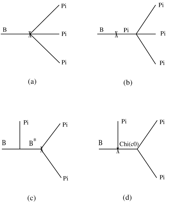
FIG. 1.: Diagrams contributing to $B^{\pm}\rightarrow\pi^{+}\pi^{-}\pi^{\pm}$. In these diagrams weak vertices are indicated by X.

REFERENCES

• [1] I.I.Bigi, B. Blok, M. Shifman, N. Uraltsev and A. Vainshtein, and references therein, in β€œB Decays”, 2nd edition, ed. S. Stone, World Scientific, 1994.
• [2] C. Quigg and J.L. Rosner, Phys. Rev. D17, 239(1978).
• [3] C. Reader and N. Isgur, Phys. Rev. D47, 1007(1993).
• [4] M. Battle et al., Phys. Rev. Lett. 71, 3922(1993).
• [5] G. Eilam, M. Gronau and R. R. Mendel, Preprint, Technion-PH-95-7, Feb. 1995.
• [6] T. Browder, K. Honscheid and S. Playfer, in Ref. 1.
• [7] M. Bauer and M. Wirbel, Z. Phys. C42, 671(1989).
• [8] M. Bauer, B. Stech and M. Wirbel, Z. Phys. C34, 1031(1987).
• [9] A. Deandrea, N. Di Bartolomeo, R. Gatto and G. Nardulli, Phys. Lett. B318, 549(1993).
• [10] Particle Data Group, Phys. Rev. D50, 1173(1994).
• [11] M.B. Wise, Caltech Preprint, CALT-68-1860, 1993. Lecture given at the CCAST Symposium on Particle Physics at the Fermi Scale (unpublished). HEP-9306277.
• [12] R. Casalbouni, A. Deandrea, N. Di Bartolomeo R. Gatto, F. Feuglio and G. Nardulli, Phys. Lett. B299, 139(1993), and references therein.
• [13] N. Isgur and M.B. Wise, Phys. Lett. B237, 527(1990).
Refer to caption