TTP 95–06

hep-ph/9503272

INCLUSIVE DECAYS
OF HEAVY FLAVOURS

Thomas Mannel

Institut für Theoretische Teilchenphysik, University of Karlsruhe
Kaiserstr. 12, D – 76128 Karlsruhe, Germany.

Recent progress in the theoretical description of inclusive heavy flavour decays is reviewed. After an outline of the theoretical methods applications to total decay rates and semileptonic decay spectra are presented.

Contribution to the workshop on “Heavy Quark Physics”,
December 13 – 16, 1994, Bad Honnef, Germany.

TTP 95–06

March 1995

1 Introduction

Decays of heavy flavours play an important role in the determination of the not yet well explored CKM sektor of the standard model. The weak processes that need to be studied involve transitions among quarks of different flavours; however, to connect the observed transitions among hadrons to the underlying quark processes one has to deal with the bound state problem of strong interactions.

For the decays of heavy flavours one may take advantage of the fact that the mass $m_{Q}$ of the heavy quark is large compared to the scale $\bar{\Lambda}$, which is determined by the light degrees of freedom and thus is of the order of $\Lambda_{QCD}$. The amplitudes or the transition rates for the decays of heavy flavoured hadrons are evaluated as an expansion in powers of $\bar{\Lambda}/m_{Q}$, the leading term of which corresponds to an infinitely heavy, static quark [1, 2, 3].

The $1/m_{Q}$ expansion has been formulated in the laguage of effective field theory, the so called Heavy Quark Effective Theory (HQET) [2, 3]. In this framework one may systematically access the mass dependence of any matrix element involving heavy hadron states and heavy quark fields. Furthermore, in the infinite mass limit two additional symmetries appear [2], which play an important role in the context of exclusive heavy flavour decays.

In the past few years methods have been developed to apply the $1/m_{Q}$ expansion also to inclusive decays of heavy hadrons [4, 5, 6, 7, 8, 9, 10], and the purpose of this talk is to give a short review of these developments. It is impossible to cover all topics in the field of inclusive decays due to length and time restrictions and consequently this review can cover only some selected topics.

For inclusive decays a $1/m_{Q}$ expansion is obtained for the rates by an approach similar to the one known from deep inelastic scattering. The first step consists of an Operator Product Expansion (OPE) which yields an infinite sum of operators with increasing dimension. The dimensions of the operators are compensated by inverse powers of a large scale, which is in general of the order of the heavy mass scale. The decay probability is then given as forward matrix elements of these operators between the state of the decaying heavy hadron; these matrix elements still have a mass dependence, which then may be extracted in terms of a $1/m_{Q}$ expansion using HQET as for exclusive decays.

In section 2 we give a short description of the OPE approach to inclusive decays. Section 3 summarizes the results for the total rates, including the first non-trivial non-perturbative corrections. In section 3 the method is applied to the charged lepton energy spectrum in inclusive semileptonic $B$ decays. It turns out that the endpoint region cannot be described by a $1/m_{Q}$ expansion; rather a partial resummation of the $1/m_{Q}$ expansion is required, which is closely analogous to the leading twist term in deep inelastic scattering [11, 12, 13, 14]. This is summarized in section 4. Finally, we conclude and point out a few open questions which are currently under study.

2 Operator Product Expansion

The effective Hamiltonian for a decay of a heavy (down-type) quark is in general linear in the decaying heavy flavoured quark

$${\cal H}_{eff}=\bar{Q}R$$ (1)

where the operator $R$ describes the decay products. In the following we shall consider semileptonic decays, for which

$$R_{sl}=\frac{G_{F}}{\sqrt{2}}V_{Qq}\,\,\gamma_{\mu}(1-\gamma_{5})q\,\,(\bar{\nu}_{\ell}\gamma^{\mu}(1-\gamma_{5})\ell),$$ (2)

where $q$ is an up-type quark ($c$ or $u$, since we shall consider $b$ decays). Similarly, for nonleptonic decays the Cabbibo allowed contribution corresponds to

$$R_{nl} = \frac{G_{F}}{2\sqrt{2}}V_{Qq}V^{*}_{q^{\prime}q^{\prime\prime}}\left[(C_{+}(m_{b})+C_{-}(m_{b}))\gamma_{\mu}(1-\gamma_{5})q\right.(\bar{q}^{\prime}\gamma^{\mu}(1-\gamma_{5})q^{\prime\prime})$$

$$\qquad\qquad\qquad+(C_{+}(m_{b})-C_{-}(m_{b}))\gamma_{\mu}(1-\gamma_{5})q^{\prime\prime}\left.(\bar{q}^{\prime}\gamma^{\mu}(1-\gamma_{5})q)\right],$$

where $q^{\prime}$ ($q^{\prime\prime}$) is a down-type (up-type) quark and $V_{Qq}$ the corresponding CKM matrix element. The coefficients $C_{\pm}(m_{b})$ are the QCD corrections obtained from the renormalization group running between $M_{W}$ and $m_{b}$; in leading logarithmic approximation these coefficients are [15]

$$C_{\pm}(m_{b})=[\frac{\alpha_{S}(M_{W}^{2})}{\alpha_{S}(m_{b}^{2})}]^{\gamma_{\pm}},\mbox{ with }\gamma_{+}=\frac{6}{33-2N_{f}}=-\frac{1}{2}\gamma_{-},$$ (4)

where $\alpha_{s}(\mu)$ is the onle-loop expression for the running coupling coupling constant of QCD.

Finally, for radiative rare decays we have

$$R_{rare}=\frac{G_{F}}{\sqrt{2}}V_{tb}V^{*}_{ts}C_{7}(m_{b})\frac{e}{16\pi^{2}}m_{b}\sigma_{\mu\nu}(1+\gamma_{5})sF^{\mu\nu},$$ (5)

where $C_{7}(m_{b})$ is again a coefficient obtained from running between $M_{W}$ and $m_{b}$. Its value is $C_{7}(m_{b})\sim 0.3$, the corresponding analytical expression may be found in [16].

The inclusive decay rate for a heavy hadron $H$ containing the quark $Q$ may be related to a forward matrix element by

$$\Gamma \propto \sum_{X}(2\pi)^{4}\delta^{4}(P_{H}-P_{X})|\langle X|{\cal H}_{eff}|H(v)\rangle|^{2}$$

$$= \int d^{4}x\,\langle H(v)|{\cal H}_{eff}(x){\cal H}_{eff}^{\dagger}(0)|H(v)\rangle$$

$$= 2\mbox{ Im}\int d^{4}x\,\langle H(v)|T\{{\cal H}_{eff}(x){\cal H}_{eff}^{\dagger}(0)\}|H(v)\rangle,$$

where $|X\rangle$ is the final state which is summed over to obtain the inclusive rate.

The matrix element appearing in (2) contains a large scale, namely the mass of the heavy quark. The first step towards a $1/m_{Q}$ expansion is to make this large scale explicit. This may be done by a phase redefinition which leads to

$$\Gamma\propto 2\mbox{ Im}\int d^{4}x\,e^{-im_{Q}vx}\langle H(v)|T\{\widetilde{{\cal H}}_{eff}(x)\widetilde{{\cal H}}_{eff}^{\dagger}(0)\}|H(v)\rangle,$$ (7)

where

$$\widetilde{{\cal H}}_{eff}=\bar{Q}_{v}R\qquad Q_{v}=e^{-im_{Q}vx}Q.$$ (8)

This relation exhibits the similarity between the cross-section calculation in deep inelastic scattering and the present approach to total rates. In deep inelastic scattering there appears a large scale which is the momentum transfer to the leptons, while here the mass of the heavy quark appears as a large scale.

The next step is to perform an operator product expansion of the product of the two Hamitonians. After the phase redefinition the remaining matrix element does not involve large momenta of the order of the heavy quark mass any more and hence a short-distance expansion becomes useful, if the mass $m_{Q}$ is large compared to the scale $\bar{\Lambda}$ determining the matrix element. The next step is thus to perform an operator-product expansion, which has the general form

$$\int d^{4}x\,e^{im_{Q}vx}\langle H(v)|T\{\widetilde{{\cal H}}_{eff}(x)\widetilde{{\cal H}}_{eff}^{\dagger}(0)\}|H(v)\rangle$$ (9)

$$\qquad\qquad=\sum_{n=0}^{\infty}\left(\frac{1}{2m_{Q}}\right)^{n}\hat{C}_{n+3}(\mu)\,\langle H(v)|{\cal O}_{n+3}|H(v)\rangle_{\mu},$$

where ${\cal O}_{n}$ are operators of dimension $n$, with their matrix elements renormalized at scale $\mu$, and $\hat{C}_{n}$ are the corresponding Wilson coefficients. These coefficients encode the short distance physics related to the heavy quark mass scale and may be calculated in perturbation theory. All long distance contributions connected to the hadronic scale $\bar{\Lambda}$ are contained in the matrix elements of the operators ${\cal O}_{n+3}$.

Still the matrix elements of ${\cal O}_{n+3}$ are not independent of the heavy quark mass scale, but this mass dependence may be expanded in powers of $1/m_{Q}$ by means of heavy quark effective theory. This is achieved by expanding the heavy quark fields appearing in the operators ${\cal O}_{n}$ as well as the states by including the corrections to the Lagrangian as time-ordered products. In this way the mass dependence of the total decay rate may be accessed completely within an expansion in $1/m_{Q}$.

The lowest-order term of the operator product expansion are the dimension-3 operators. Due to Lorentz invariance and parity there are only two combinations which may appear, namely $\bar{Q}_{v}\mathchoice{\ooalign{$\hfil\displaystyle\mkern 0.0mu/\hfil$\crcr$\displaystyle v$}}{\ooalign{$\hfil\textstyle\mkern 0.0mu/\hfil$\crcr$\textstyle v$}}{\ooalign{$\hfil\scriptstyle\mkern 0.0mu/\hfil$\crcr$\scriptstyle v$}}{\ooalign{$\hfil\scriptscriptstyle\mkern 0.0mu/\hfil$\crcr$\scriptscriptstyle v$}}Q_{v}$ or $\bar{Q}_{v}Q_{v}$. Note that the $Q_{v}$ operators differ from the full QCD operators only by a phase redefinition, and hence $\bar{Q}_{v}\mathchoice{\ooalign{$\hfil\displaystyle\mkern 0.0mu/\hfil$\crcr$\displaystyle v$}}{\ooalign{$\hfil\textstyle\mkern 0.0mu/\hfil$\crcr$\textstyle v$}}{\ooalign{$\hfil\scriptstyle\mkern 0.0mu/\hfil$\crcr$\scriptstyle v$}}{\ooalign{$\hfil\scriptscriptstyle\mkern 0.0mu/\hfil$\crcr$\scriptscriptstyle v$}}Q_{v}=\bar{Q}\mathchoice{\ooalign{$\hfil\displaystyle\mkern 0.0mu/\hfil$\crcr$\displaystyle v$}}{\ooalign{$\hfil\textstyle\mkern 0.0mu/\hfil$\crcr$\textstyle v$}}{\ooalign{$\hfil\scriptstyle\mkern 0.0mu/\hfil$\crcr$\scriptstyle v$}}{\ooalign{$\hfil\scriptscriptstyle\mkern 0.0mu/\hfil$\crcr$\scriptscriptstyle v$}}Q$ and $\bar{Q}_{v}Q_{v}=\bar{Q}Q$. The first combination is proportional to the $Q$-number current $\bar{Q}\gamma_{\mu}Q$, which is normalized even in full QCD, while the second differs from the first one only by terms of order $1/m_{Q}^{2}$

$$\bar{Q}_{v}Q_{v}=v_{\mu}\bar{Q}_{v}\gamma_{\mu}Q_{v}+\frac{1}{2m_{Q}^{2}}\bar{h}_{v}\left[(iD)^{2}-(ivD)^{2}+\frac{i}{2}\sigma_{\mu\nu}G^{\mu\nu}\right]h_{v}+{\cal O}(1/m_{Q}^{3}),$$ (10)

where $G_{\mu\nu}$ is the gluon field strength.

Thus the matrix elements of the dimension-3 contribution is known to be normalized; in the standard normalization of the states this implies

$$\langle H(v)|{\cal O}_{3}|H(v)\rangle=\langle H(v)|\bar{Q}_{v}\mathchoice{\ooalign{$\hfil\displaystyle\mkern 0.0mu/\hfil$\crcr$\displaystyle v$}}{\ooalign{$\hfil\textstyle\mkern 0.0mu/\hfil$\crcr$\textstyle v$}}{\ooalign{$\hfil\scriptstyle\mkern 0.0mu/\hfil$\crcr$\scriptstyle v$}}{\ooalign{$\hfil\scriptscriptstyle\mkern 0.0mu/\hfil$\crcr$\scriptscriptstyle v$}}Q_{v}|H(v)\rangle=2m_{H},$$ (11)

where $m_{H}$ is the mass of the heavy hadron. To lowest order in the heavy mass expansion we may furthermore replace $m_{H}=m_{Q}$ and hence we may evaluate the leading term in the $1/m_{Q}$ expansion without any hadronic uncertainty. Generically the dimension-3 contribution yields the free quark decay rate. This has been previously used as a model for inclusive decays, but now it turns out to be the first term in a systematic $1/m_{Q}$ expansion of total rates.

A dimension-4 operators contains an additional covariant derivative, and thus one has matrix elements of the type

$$\langle H(v)|{\cal O}_{4}|H(v)\rangle\propto\langle H(v)|\bar{Q}_{v}\Gamma D_{\mu}Q_{v}|H(v)\rangle={\cal A}_{\Gamma}v_{\mu}{}.$$ (12)

Since the equations of motion apply for this tree level matrix element, one finds that the constant ${\cal A}_{\Gamma}$ has to vanish, and thus there are no dimension-4 contributions. This statement is completely equivalent to Lukes theorem [17], since we are considering a forward matrix element, i.e. a matrix element at zero recoil [18].

The first non-trivial non-perturbative contribution comes from dimension-5 operators and are of order $1/m_{Q}^{2}$. For mesonic decays there are only the two parameters $\lambda_{1}$ and $\lambda_{2}$ corresponding to matrix elements involving higher order terms that appear in the effective theory Lagrangian

$$\lambda_{1} = \frac{\langle H(v)|\bar{h}_{v}(iD)^{2}h_{v}|H(v)\rangle}{2M_{H}}$$ (13)

$$\lambda_{2} = \frac{\langle H(v)|\bar{h}_{v}\sigma_{\mu\nu}iD^{\mu}iD^{\nu}h_{v}|H(v)\rangle}{2M_{H}},$$ (14)

where the normalization of the states is chosen to be $\langle H(v)|\bar{h}_{v}h_{v}|H(v)\rangle=2M_{H}$, where $M_{H}$ is the mass of the heavy meson in the static limit. These parameters may be interpreted as the expectation value of the kinetic energy of the heavy quark and its energy due to the chromomagnetic moment of the heavy quark inside the heavy meson respectively.

The parameter $\lambda_{2}$ is easy to access, since it is related to the mass splitting between $H(v)$ and $H^{*}(v,\epsilon)$. From the $B$-meson system we obtain

$$\lambda_{2}(m_{b})=\frac{1}{4}(M_{H^{*}}-M_{H})=0.12\mbox{ GeV}^{2};$$ (15)

from the charm system the same value is obtained. This shows that indeed the spin-symmetry partners are degenerate in the infinite mass limit and the splitting between them scales as $1/m_{Q}$.

The parameter $\lambda_{1}$ appearing is not simply related to the hadron spectrum; from the definition of $\lambda_{1}$ one is led to assume $\lambda_{1}<0$; a more restrictive inequality

$$-\lambda_{1}>3\lambda_{2}$$ (16)

has been derived in a quantum mechanical framework in [12] and using heavy-flavour sum rules [19]. Furthermore, there exists also a QCD sum rule estimate [20] for this parameter:

$$\lambda_{1}=-0.52\pm 0.12\mbox{ GeV}^{2}.$$ (17)

3 Total Decay Rates

In this section we collect the results for the total rates including the first non-trivial non-perturbative correction.

Inserting $R_{sl}$ as given in (2) one obtains for the total inclusive semileptonic decay rate $B\to X_{c}\ell\nu$

$$\Gamma_{B\to X_{c}\ell\nu}=\frac{G_{F}^{2}m_{b}^{5}}{192\pi^{3}}|V_{cb}|^{2}\left[\left(1+\frac{\lambda_{1}}{2m_{c}^{2}}\right)f_{1}\left(\frac{m_{c}}{m_{b}}\right)-\frac{9\lambda_{2}}{2m_{c}^{2}}f_{2}\left(\frac{m_{c}}{m_{b}}\right)\right],$$ (18)

where the two $f_{j}$ are phase-space functions

$$f_{1}(x) = 1-8x^{2}+8x^{6}-x^{8}-24x^{4}\log x,$$ (19)

$$f_{2}(x) = 1-\frac{8}{3}x^{2}-8x^{4}+8x^{6}+\frac{5}{3}x^{8}+8x^{4}\log x.$$

The result for $B\to X_{u}\ell\nu_{\ell}$ is obtained from (18) as the limit $m_{c}\to 0$ and the replacement $V_{cb}\to V_{ub}$

$$\Gamma_{B\to X_{u}\ell\nu}=\frac{G_{F}^{2}m_{b}^{5}}{192\pi^{3}}|V_{ub}|^{2}\left[1+\frac{\lambda_{1}-9\lambda_{2}}{2m_{b}^{2}}\right].$$ (20)

As was discussed above, the leading non-perturbative corrections in (18) and (20) are parametrized by $\lambda_{1}$ and $\lambda_{2}$. Estimates for these parameters have been discussed in section 2; in order to estimate the total effect of the non-perturbative effects we insert a range of values $-0.3>\lambda_{1}>-0.6$ GeV²; from this we obtain

$$\frac{\lambda_{1}-9\lambda_{2}}{2m_{b}^{2}}\sim-(3\cdots 4)\%$$ (21)

This means that the non-perturbative contributions are small, in particular compared to the perturbative ones, which have been calculated some time ago [21, 22]. For the decay $B\to X_{u}\ell\bar{\nu}_{\ell}$ the lowest order QCD corrections are given by

$$\Gamma_{B\to X_{u}\ell\bar{\nu}_{\ell}}=\frac{G_{F}^{2}m_{b}^{5}}{192\pi^{3}}|V_{ub}|^{2}\left[1+\frac{2\alpha}{3\pi}\left(\frac{25}{4}-\pi^{2}\right)\right]=0.85|V_{ub}|^{2}\Gamma_{b},$$ (22)

and thus the typical size of QCD radiative corrections is of the order of ten to twenty percent.

Similarly, one obtains the result for non-leptonic decays as

$$\Gamma_{X_{c}}=3\frac{G_{F}^{2}m_{b}^{5}}{192\pi^{3}}\left\{A_{1}f_{1}\left(\frac{m_{c}}{m_{b}}\right)\left[1+\frac{1}{2m_{b}^{2}}(\lambda_{1}-9\lambda_{2})\right]-48A_{2}f_{3}\left(\frac{m_{c}}{m_{b}}\right)\frac{1}{2m_{b}^{2}}\lambda_{2}\right\},$$ (23)

where the coefficients $A_{i}$ are expressed as combination of the Wilson coefficents $C_{\pm}(m_{b})$ given in (4)

$$A_{1}=\frac{1}{3}[C_{-}^{2}(m_{b})+2C_{+}^{2}(m_{b})],\qquad A_{2}=\frac{1}{6}[C_{+}^{2}(m_{b})-C_{-}^{2}(m_{b})],$$ (24)

and $f_{3}(x)=(1-x^{2})^{3}$ is another phase space function. Again the non-perturbative corrections turn out to be small, in the region of a few percent compared to the leading term, and the perturbative corrections turn out to be much larger than this.

Finally, for the rare decay $B\to X_{s}\gamma$ one may as well calculate the non-perturbative contribution in terms of $\lambda_{1}$ and $\lambda_{2}$. One obtains

$$\Gamma_{B\to X_{s}\gamma}=\frac{\alpha G_{F}^{2}}{16\pi^{4}}m_{b}^{5}|V_{ts}V_{td}^{*}|^{2}|C_{7}(m_{b})|^{2}\left[1+\frac{1}{2m_{b}^{2}}\left(\lambda_{1}-9\lambda_{2}\right)\right],$$ (25)

and the relative size of the nonperturbative corrections is the same as in the $B\to X_{u}\ell\bar{\nu}_{\ell}$ decays.

Typically the non-pertubative corrections are much smaller than the radiative corrections. The only exception is the endpoint region of lepton energy spectra which receives both large perturbative as well as nonperturbative corrections. However, this is only a small region in phase space and the corrections to the total rates remain moderate.

4 Lepton Energy Spectra

The method of the operator-product expansion may also be used to obtain the non-perturbative corrections to the charged lepton energy spectrum. In this case the operator product expansion is applied not to the full effective Hamiltonian, but rather only to the hadronic currents. The rate is written as a product of the hadronic and leptonic tensor

$$d\Gamma=\frac{G_{F}^{2}}{4m_{B}}|V_{Qq}|^{2}W_{\mu\nu}\Lambda^{\mu\nu}d(PS),$$ (26)

where $d(PS)$ is the phase-space differential. The short-distance expansion is then performed for the two currents appearing in the hadronic tensor. Redefining the phase of the heavy-quark fields as in (8) one finds that the momentum transfer variable relevant for the short-distance expansion is $m_{Q}v-q$, where $q$ is the momentum transfer to the leptons.

The structure of the expansion for the spectrum is identical to the one of the total rate. The contribution of the dimension-3 operators yields the free-quark decay spectrum, there are no contributions from dimension-4 operators, and the $1/m_{b}^{2}$ corrections are parametrized in terms of $\lambda_{1}$ and $\lambda_{2}$. Calculating the spectrum for $B\to X_{c}\ell\nu$ yields [6, 7, 8, 9]

$$\frac{d\Gamma}{dy} = \frac{G_{F}^{2}\,|\,V_{cb}|^{2}\,m_{b}^{5}}{192\pi^{3}}\Theta(1-y-\rho)y^{2}\left[\left\{3(1-\rho)(1-R^{2})-2y(1-R^{3})\right\}\right.$$

$$+\frac{\lambda_{1}}{[m_{b}(1-y)]^{2}}(3R^{2}-4R^{3})-\frac{\lambda_{1}}{m_{b}^{2}(1-y)}(R^{2}-2R^{3})$$

$$-\frac{3\lambda_{2}}{m_{b}^{2}(1-y)}(2R+3R^{2}-5R^{3})+\frac{\lambda_{1}}{3m_{b}^{2}}[5y-2(3-\rho)R^{2}+4R^{3}]$$

$$\left.+\frac{\lambda_{2}}{m_{b}^{2}}[(6+5y)-12R-(9-5\rho)R^{2}+10R^{3}]\right]+{\cal O}\left[(\Lambda/[m_{b}(1-y)])^{3}\right],$$

where we have defined

$$\rho=\left(\frac{m_{c}}{m_{b}}\right)^{2},\quad R=\frac{\rho}{1-y}$$ (28)

and

$$y=2E_{\ell}/m_{b}$$ (29)

is the rescaled energy of the charged lepton.

This expression is somewhat complicated, but it simplifies for the decay $B\to X_{u}\ell\nu$ since then the mass of the quark in the final state may be neglected. One finds

$$\frac{d\Gamma}{dy} = \frac{G_{F}^{2}\,|\,V_{ub}|^{2}\,m_{b}^{5}}{192\pi^{3}}\left[\left(2y^{2}(3-2y)+\frac{10y^{2}}{3}\frac{\lambda_{1}}{m_{b}^{2}}+2y(6+5y)\frac{\lambda_{2}}{m_{b}^{2}}\right)\Theta(1-y)\right.$$ (30)

$$\vphantom{\frac{G_{F}^{2}\,|\,V_{qb}|^{2}\,m_{b}^{5}}{192\pi^{3}}}\left.-\frac{\lambda_{1}+33\lambda_{2}}{3m_{b}^{2}}\delta(1-y)-\frac{\lambda_{1}}{3m_{b}^{2}}\delta^{\prime}(1-y)\right].$$

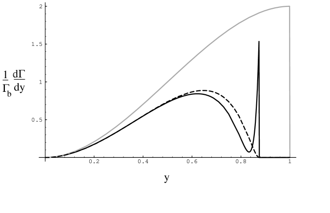
Figure 1: The electron spectrum for free quark $b\rightarrow c$ decay (dashed line), free quark $b\rightarrow u$ decay (grey line), and $B\rightarrow X_{c}e\bar{\nu}_{e}$ decay including $1/m_{b}^{2}$ corrections (solid line) with $\lambda_{1}=-0.5$ GeV² and $\lambda_{2}=0.12$ GeV². The figure is from [8].

Figure 1 shows the distributions for inclusive semileptonic decays of $B$ mesons. The spectrum close to the endpoint, where the lepton energy becomes maximal, exhibits a sharp spike as $y\to y_{max}$. In this region we have

$$\frac{d\Gamma}{dy}\propto\Theta(1-y-\rho)\left[2+\frac{\lambda_{1}}{(m_{Q}(1-y))^{2}}\left(\frac{\rho}{1-\rho}\right)^{2}\left\{3-4\left(\frac{\rho}{1-\rho}\right)\right\}\right],$$ (31)

which behaves like $\delta$-functions and its derivatives as $\rho\to 0$, which can be seen in (30). This behaviour indicates a breakdown of the operator product expansion close to the endpoint, since for the spectra the expansion parameter is not $1/m_{Q}$, but rather $1/(m_{Q}-qv)$, which becomes $1/(m_{Q}[1-y])$ after the integration over the neutrino momentum. In order to obtain a description of the endpoint region, one has to perform some resummation of the operator product expansion.

5 Resummation in the Endpoint Region

Very close to the endpoint of the inclusive semileptonic decay spectra only a few resonances contribute. In this resonance region one cannot expect to have a good description of the spectrum using an approach based on parton-hadron duality; here a sum over a few resonances will be appropriate.

In the variable $y$ the size of this resonance region is, however, of the order of $(\bar{\Lambda}/m_{Q})^{2}$ and thus small. In a larger region of the order $\bar{\Lambda}/m_{Q}$, which we shall call the endpoint region, many resonances contribute and one may hope to describe the spectrum in this region using parton-hadron duality.

It has been argued in [11] that the $\delta$-function-like singularities appearing in (30) may be reinterpreted as the expansion of a non-perturbative function describing the spectrum in the endpoint region. Keeping only the singular terms of (30) we write

$$\frac{1}{\Gamma_{b}}\frac{d\Gamma}{dy}=2y^{2}(3-2y)S(y),$$ (32)

where

$$S(y)=\Theta(1-y)+\sum_{n=0}^{\infty}a_{n}\delta^{(n)}(1-y)$$ (33)

is a non-perturbative function given in terms of the moments $a_{n}$ of the spectrum, taken over the endpoint region. These moments themselves have an expansion in $1/m_{Q}$ such that $a_{n}\sim 1/m_{Q}^{n+1}$, and we shall consider only the leading term in the expansion of the moments, corresponding to the most singular contribution to the endpoint region.

Comparing (30) with (32) and (33) one obtains that

$$a_{0} = \int dy(S(y)-\Theta(1-y))={\cal O}(1/m_{Q}^{2}),$$ (34)

$$a_{1} = \int y(S(y)-\Theta(1-y))=-\frac{\lambda_{1}}{3m_{Q}^{2}},$$ (35)

where the integral extends over the endpoint region.

The non-perturbative function implements a resummation of the most singular terms contributing to the endpoint and, in the language of deep inelastic scattering, corresponds to the leading twist contribution. A similar approach based on the parton model will be described in a separate talk at this conference [23].

This resummation has been studied in QCD [12, 13] and the function $S(y)$ may be related to the distribution of the light cone component of the heavy quark residual momentum inside the heavy meson. The latter is a fundamental function for inclusive heavy-to-light transitions, which has been defined in [12]

$$f(k_{+})=\frac{1}{2m_{B}}\langle H(v)|\,\bar{h}_{v}\,\delta(k_{+}-iD_{+})\,h_{v}\,|H(v)\rangle,$$ (36)

where $k_{+}=k_{0}+k_{3}$ is the positive light cone component of the residual momentum $k$. The relation between the two functions $S$ and $f$ is given by

$$S(y)=\frac{1}{m_{Q}}\int\limits_{-m_{Q}(1-y)}^{\bar{\Lambda}}dk_{+}f(k_{+}),$$ (37)

from which we infer that the $n^{th}$ moment of the endpoint region is given in terms of the matrix element $\langle B(v)|\bar{h}_{v}(iD_{+})^{n}h_{v}|B(v)\rangle$.

The function $f$ is a universal distribution function, which appears in all heavy-to-light inclusive decays; another example is the decay $B\to X_{s}\gamma$ [14, 12], where this function determines the photon-energy spectrum in a region of order $1/m_{Q}$ around the $K^{*}$ peak.

In principle $f$ has to be determined by other methods than the $1/m_{Q}$ expansion, e.g. from lattice calculations or from a model, or it has to be determined from experiment by measuring the photon spectrum in $B\to X_{s}\gamma$ or the lepton spectrum in $B\to X_{u}\ell\bar{\nu}$. In the context of the model ACCMM model [22] $f$ has been calculated in [24].

Some of the properties of $f$ are known. Its support is $-\infty<k_{+}<\bar{\Lambda}$, it is normalized to unity, and its first moment vanishes. Its second moment is given by $a_{1}$, and its third moment has been estimated [12, 18]. A one-parameter model for $f$ has been suggested in [13], which incorporates the known features of $f$

$$f(k_{+})={32\over\pi^{2}\bar{\Lambda}}\,(1-x)^{2}\exp\bigg{\{}-{4\over\pi}\,(1-x)^{2}\bigg{\}}\,\Theta(1-x),$$ (38)

where $x=k_{+}/\bar{\Lambda}$, and the choice $\bar{\Lambda}=570$ MeV yields reasonable values for the moments. In fig. 2 we show the spectrum for $B\to X_{u}\ell\nu_{\ell}$ using the ansatz (38).

Figure 2: Charged-lepton spectrum in $B\to X_{u}\ell\bar{\nu}$ decays. The solid line is (32) with the ansatz (38), the dashed line shows the prediction of the free-quark decay model. The figure is from [13].

Including the non-perturbative effects yields a reasonably behaved spectrum in the endpoint region and the $\delta$-function-like singularities have disappeared. Furthermore, the spectrum now extends beyond the parton model endpoint; it is shifted from $E_{\ell}^{max}=m_{Q}/2$ to the physical endpoint $E_{\ell}^{max}=M_{H}/2$, since $f$ is non-vanishing for positive values of $k_{+}<\bar{\Lambda}=M_{H}-m_{Q}$.

6 Conclusions and Open Questions

The $1/m_{Q}$ expansion obtained from the OPE and HQET offers the unique possibility to calculate the transition rates for inclusive decays in a QCD based and model independent framework. The leading term of this expansion is always the free quark decay, and the first non-trivial corrections are in general given by the mean kinetic energy of the heavy quark inside the heavy hadron $\lambda_{1}$ and the matrix element $\lambda_{2}$ of the chromomagnetic moment operator.

The method also allows us to calculate differential distributions, such as the charged lepton energy spectrum in inclusive semileptonic decays of heavy hadrons. For this case, the expansion parameter is the inverse of the energy release $m_{b}-2E_{\ell}$, where $E_{\ell}$ is the lepton energy. Close to the endpoint, the energy release is small and thus the expansion in its inverse powers becomes useless. In this kinematic region one may partially resume the $1/m_{Q}$ expansion, obtaining a result closely analogous to the leading twist term in deep inelastic scattering. Particularly in the endpoint region a non-perturbative function is needed which corresponds to the parton distributions parametrizing the deep inelastic scattering.

The main focus of this review have been the non-perturbative corrections, and we did not consider the perturbative ones. In general, the non-perturbative contributions are typically a few percent, while the perturbative ones are usually in excess of ten percent. An exception is the endpoint region of semileptonic decay spectra, where both the perturbative and the non-perturbative corrections become large and it becomes hard to disentangle the two.

The method of the $1/m_{Q}$ expansion allows us to systematically calculate even purely hadronic inclusive rates. This is remarkable, since calculations of exclusive hadronic processes are still very model dependent and thus in general not reliable. Having control over the purely hadronic inclusive widths means that one is in the position to calculate lifetimes and branching fractions within the $1/m_{Q}$ expansion.

The leading term of the $1/m_{Q}$ expansion is the free quark decay, and it is known that the semileptonic branching fraction calculated in the parton model is too large by a few percent. The first non-perturbative corrections turn out to be much too small to explain the low semileptonic branching fraction. The perturbative corrections are larger and indeed tend to lower the semileptonic branching fraction, but the effect is still too small to explain the data. Recent calculations [25, 26] indicate that there are some effects originating from the finite mass of the final state quarks, in particular in the channel $b\to c\bar{c}s$. However, enlarging this channel relative to $b\to c\bar{u}d$ will increase the average number $n_{c}$ of charm quarks produced per $b$ decay. Experimentally, $n_{c}$ is close to unity, $n_{c}=1.04\pm 0.07$ [27], while an explanation of the low semileptonic branching fraction via an enhancement of the channel $b\to c\bar{c}s$ would lead to $n_{c}\sim 1.3$.

The problem of the semileptonic branching fraction is at the level of a two standard deviation discrepancy, and another problem of about the same significance are the lifetimes of $b$ hadrons. Lifetime differences between $B$ mesons should show up a the level of the $1/m_{b}^{3}$ corrections and thus should be small. This is supported by data; however, the situation is different for the lifetime of $b$ baryons. Their lifetime may differ at the $1/m_{b}^{2}$ level and hence are expected to be of the order of a few percent. Experimentally one finds a large lifetime difference between the $\Lambda_{b}$ and the $B$ mesons: $\tau(\Lambda_{b})/\tau(B_{d})=0.72\pm 0.11$.

If with new and improved data these two problems persist, they will need clarification and perhaps will lead to new insights into the strong interaction aspects of heavy flavour weak decays.

References

- [1] M. Voloshin and M. Shifman, Sov. J. Nucl. Phys. 45 (1987) 292 and 47 (1988) 511; E. Eichten and B. Hill, Phys. Lett. B234 (1990) 511; a more complete set of references can be found in one of the reviews [3].
- [2] N. Isgur and M. Wise, Phys. Lett. B232 (1989) 113 and B237 (1990) 527; B. Grinstein, Nucl. Phys. B339 (1990) 253; H. Georgi, Phys. Lett. B240 (1990) 447; A. Falk, H. Georgi, B. Grinstein and M. Wise, Nucl. Phys. B343 (1990) 1.
- [3] The subject of HQET is reviewed in: H. Georgi: contribution to the Proceedings of TASI–91, by R. K. Ellis et al. (eds.) (World Scientific, Singapore, 1991); B. Grinstein: contribution to High Energy Phenomenology, R. Huerta and M. A. Peres (eds.) (World Scientific, Singapore, 1991); N. Isgur and M. Wise: contribution to Heavy Flavors, A. Buras and M. Lindner (eds.) (World Scientific, Singapore, 1992); M. Neubert, Phys. Rept. 245 (1994) 259; T. Mannel, contribution to QCD–20 years later, P. Zerwas and H. Kastrup (eds.) (World Scientific, Singapore 1993).
- [4] M. Shifman and M. Voloshin, Sov. J. Nucl. Phys. 41 (1985) 120; V. Khoze et al., Sov. J. Nucl. Phys. 46 (1987) 112.
- [5] J. Chay, H. Georgi and B. Grinstein, Phys. Lett. B247 (1990) 399.
- [6] I. Bigi, N. Uraltsev and A. Vainshtein, Phys. Lett. B293 (1992) 430; I. Bigi et al., Minnesota TPI-MINN-92/67-T (1992) and Phys. Rev. Lett. 71 (1993) 496.
- [7] B. Blok et al., Phys. Rev. D49 (1994) 3356.
- [8] A. Manohar and M. Wise, Phys. Rev. D49 (1994) 1310.
- [9] T. Mannel, Nucl. Phys. B423 (1994) 396.
- [10] A. Falk, M. Luke and M. Savage, Phys. Rev. D49 (1994) 3367.
- [11] M. Neubert, Phys. Rev. D49 (1994) 2472.
- [12] I. Bigi et al., Int. J. Mod. Phys. A9 (1994) 2467.
- [13] T. Mannel and M. Neubert, preprint CERN-TH.7156/94 (1994).
- [14] M. Neubert, Phys. Rev. D49 (1994) 4623.
- [15] F. Gilman and M. Wise, Phys. Rev. D20 (1979) 2392; A. Buras et al., Nucl. Phys. B370 (1992) 69.
- [16] B. Grinstein, R. Springer and M. Wise, Nucl. Phys. B319 (1988) 271; M. Misiak, Nucl. Phys. B393 (1993) 23.
- [17] M. Luke, Phys. Lett. B252 (1990) 447.
- [18] T. Mannel, Phys. Rev. D50 (1994) 428.
- [19] I. Bigi et al., preprint CERN-TH-7250/94 (1994), hep-ph/9405410.
- [20] P. Ball and V. Braun, Phys. Rev. D49 (1994) 2472.
- [21] A. Ali and E. Pietarinen, Nucl. Phys. B154 (1979) 519; N. Cabibbo, G. Corbo and L. Maiani, Nucl. Phys. B155 (1979) 83; G. Corbo, Nucl. Phys. B212 (1983) 99; M. Jezabek and J. H. Kühn, Nucl. Phys. B320 (1989) 20; A. Falk et al., Phys. Rev. D49 (1994) 3367.
- [22] G. Altarelli et al., Nucl. Phys. B208 (1982) 365.
- [23] E. Paschos, contribution to this conference, C. Jin, W. Palmer and E. Paschos, Phys. Lett. B329 (1994) 364.
- [24] I. Bigi et al, preprint CERN-TH.7159/94.
- [25] E. Bagan et al., Phys. Lett. B342 (1995) 362.
- [26] E. Bagan et al., preprint CERN-TH.95–25.
- [27] P. Roudeau, Rapporteur talk at the ICHEP 94 Conference, Glasgow, Scottland.