FTUV/94-62

IFIC/94-59

hep-ph/9412274

THE STANDARD MODEL OF
ELECTROWEAK INTERACTIONS

A. Pich

Departament de Física Teòrica and IFIC, Universitat de València – CSIC

Dr. Moliner 50, E–46100 Burjassot, València, Spain

Abstract

What follows is an updated version of the lectures given at the CERN Academic Training (November 1993) and at the Jaca Winter Meeting (February 1994). The aim is to provide a pedagogical introduction to the Standard Model of electroweak interactions. After briefly reviewing the empirical considerations which lead to the construction of the Standard Model Lagrangian, the particle content, structure and symmetries of the theory are discussed. Special emphasis is given to the many phenomenological tests (universality, flavour-changing neutral currents, precision measurements, quark mixing, etc.) which have established this theoretical framework as the Standard Theory of electroweak interactions.

Lectures given at the XXII International Winter Meeting on Fundamental Physics,

The Standard Model and Beyond, Jaca (Spain), 7-11 February 1994,

and at the

CERN Academic Training, Geneva (Switzerland), 15-26 November 1993

FTUV/94-62

IFIC/94-59

November 1994

1 Introduction

The Standard Model (SM) is a gauge theory, based on the group $SU(3)_{C}\otimes SU(2)_{L}\otimes U(1)_{Y}$, which describes strong, weak and electromagnetic interactions, via the exchange of the corresponding spin–1 gauge fields: 8 massless gluons and 1 massless photon for the strong and electromagnetic interactions, respectively, and 3 massive bosons, $W^{\pm}$ and $Z$, for the weak interaction. The fermionic-matter content is given by the known leptons and quarks, which are organized in a 3–fold family structure:

$$\left[\begin{array}[]{cc}\nu_{e}&u\\ e^{-}&d\end{array}\right]\,,\qquad\quad\left[\begin{array}[]{cc}\nu_{\mu}&c\\ \mu^{-}&s\end{array}\right]\,,\qquad\quad\left[\begin{array}[]{cc}\nu_{\tau}&t\\ \tau^{-}&b\end{array}\right]\,,$$ (1.1)

where (each quark appears in 3 different “colours”)

$$\left[\begin{array}[]{cc}\nu_{l}&q_{u}\\ l^{-}&q_{d}\end{array}\right]\,\,\equiv\,\,\left(\begin{array}[]{c}\nu_{l}\\ l^{-}\end{array}\right)_{L},\quad\left(\begin{array}[]{c}q_{u}\\ q_{d}\end{array}\right)_{L},\quad l^{-}_{R},\quad(q_{u})_{R},\quad(q_{d})_{R},$$ (1.2)

plus the corresponding antiparticles. Thus, the left-handed fields are $SU(2)_{L}$ doublets, while their right-handed partners transform as $SU(2)_{L}$ singlets. The 3 fermionic families in Eq. (1.1) appear to have identical properties (gauge interactions); they only differ by their mass and their flavour quantum number.

The gauge symmetry is broken by the vacuum, which triggers the Spontaneous Symmetry Breaking (SSB) of the electroweak group to the electromagnetic subgroup:

$$SU(3)_{C}\otimes SU(2)_{L}\otimes U(1)_{Y}\,\stackrel{{\scriptstyle\mbox{\rm\scriptsize SSB}}}{{\longrightarrow}}\,SU(3)_{C}\otimes U(1)_{QED}\,.$$ (1.3)

The SSB mechanism generates the masses of the weak gauge bosons, and gives rise to the appearance of a physical scalar particle in the model, the so-called “Higgs”.

The SM constitutes one of the most successful achievements in modern physics. It provides a very elegant theoretical framework, which is able to describe all known experimental facts in particle physics.

These lectures provide an introduction to the electroweak sector of the SM, i.e. the $SU(2)_{L}\otimes U(1)_{Y}$ part [1, 2, 3, 4] (the strong $SU(3)_{C}$ piece is discussed in Ref. [5]). Sects. 2 and 3 describe some experimental and theoretical arguments suggesting the structure presented above [Eqs. (1.1) to (1.3)] as the natural model for describing the electroweak interactions. The power of the gauge principle is shown in Sect. 4, in the simpler QED case. The SM framework is presented in Sects. 5, 6 and 8, which discuss the gauge structure, the SSB mechanism and the family structure, respectively. Some further theoretical considerations concerning quantum anomalies are given in Sect. 7. Sects. 9 to 12 summarize the present phenomenological status of the SM. A few comments on open questions, to be tested at future facilities, are finally given in Sect. 13.

2 Low-Energy Experimental Facts

2.1 $\mu^{-}\to e^{-}\bar{\nu}_{e}\nu_{\mu}$ decay

Let us parametrize the 3–body decay of the muon by a general local, derivative-free, 4–fermion Hamiltonian:

$${\cal H}_{\mbox{\rm\scriptsize eff}}\,=\,\sum_{n,\epsilon,\omega}\,g^{n}_{\epsilon,\omega}\,\left[\bar{e}_{\epsilon}\Gamma^{n}(\nu_{e})_{\sigma}\right]\,\left[(\bar{\nu}_{\mu})_{\lambda}\Gamma_{n}\mu_{\omega}\right]\,.$$ (2.1)

Here, $\epsilon,\omega,\sigma,\lambda$ denote the chiralities (left-handed, right-handed) of the corresponding fermions, and $n$ labels the type on interaction: scalar ($I$), vector ($\gamma^{\mu}$), tensor($\sigma^{\mu\nu}$). For given $n,\epsilon,\omega$, the neutrino chiralities $\sigma$ and $\lambda$ are uniquely determined.

The couplings $g^{n}_{\epsilon,\omega}$ can be determined experimentally, by studying the energy and angular (with respect to the $\mu^{-}$-spin) distribution of the final electron, the $e^{-}$ polarization, and the cross-section of the related $\nu_{\mu}e^{-}\to\mu^{-}\nu_{e}$ process. One finds that the decay amplitude involves only left-handed fermions, with an effective Hamiltonian of the $V-A$ type:

$${\cal H}_{\mbox{\rm\scriptsize eff}}\,=\,{G_{F}\over\sqrt{2}}\left[\bar{e}\gamma^{\alpha}(1-\gamma_{5})\nu_{e}\right]\,\left[\bar{\nu}_{\mu}\gamma_{\alpha}(1-\gamma_{5})\mu\right]\,.$$ (2.2)

The so-called Fermi coupling constant $G_{F}$ is fixed by the total decay width,

$${1\over\tau_{\mu}}\,=\,\Gamma(\mu^{-}\to e^{-}\bar{\nu}_{e}\nu_{\mu})\,=\,{G_{F}^{2}m_{\mu}^{5}\over 192\pi^{3}}\,\left(1+\delta_{\mbox{\rm\scriptsize QED}}\right)\,f\left({m_{e}^{2}\over m_{\mu}^{2}}\right)\,,$$ (2.3)

where $\,f(x)=1-8x+8x^{3}-x^{4}-12x^{2}\ln{x}$, and $\,\delta_{\mbox{\rm\scriptsize QED}}={\alpha\over 2\pi}\left({25\over 4}-\pi^{2}\right)\approx-0.0042\,$ takes into account the leading radiative QED corrections [7]. From the measured lifetime [8], $\tau_{\mu}=(2.19703\pm 0.00004)\times 10^{-6}$ s, one gets the value

$$G_{F}\,=\,(1.16639\pm 0.00002)\times 10^{-5}\,\mbox{\rm GeV}^{-2}\,\approx\,{1\over(293\,\mbox{\rm GeV})^{2}}\,.$$ (2.4)

2.2 Beta decay

The weak transitions $d\to ue^{-}\bar{\nu}_{e}$ and $u\to de^{+}\nu_{e}$ can be studied through the corresponding hadronic decays $n\to pe^{-}\bar{\nu}_{e}$ and $p\to ne^{+}\nu_{e}$, where the last process can only occur within a nuclear transition because it is kinematically forbidden for a free proton. The experimental analysis of these processes shows that they can be described by the effective Hamiltonian

$${\cal H}_{\mbox{\rm\scriptsize eff}}\,=\,{G^{\Delta S=0}\over\sqrt{2}}\left[\bar{p}\gamma^{\alpha}(1-g_{A}\gamma_{5})n\right]\,\left[\bar{e}\gamma_{\alpha}(1-\gamma_{5})\nu_{e}\right]\,,$$ (2.5)

where [8]

$$G^{\Delta S=0}\,\approx\,0.975\,G_{F}\,,\qquad\qquad g_{A}\,=\,1.2573\pm 0.0028\,.$$ (2.6)

The strength of the interaction turns out to be approximately the same as for $\mu$ decay and, again, only left-handed leptons are involved. The strong similarity with Eq. (2.2) suggest a universal (same type and strength) interaction at the quark-lepton level:

$${\cal H}_{\mbox{\rm\scriptsize eff}}\,=\,{G^{\Delta S=0}\over\sqrt{2}}\left[\bar{u}\gamma^{\alpha}(1-\gamma_{5})d\right]\,\left[\bar{e}\gamma_{\alpha}(1-\gamma_{5})\nu_{e}\right]\,.$$ (2.7)

In fact, the conservation of the vector current, $\partial_{\mu}\left(\bar{u}\gamma^{\mu}d\right)=0$, implies $\,\langle p|\bar{u}\gamma^{\mu}d|n\rangle=\bar{p}\gamma^{\mu}n\,$ at $q^{2}=0$; i.e. strong interactions do not renormalize the vector current. However, the axial-current matrix elements do get modified by the QCD dynamics. Thus, the factor $g_{A}$ can be easily understood as a QCD effect. The interaction (2.7) correctly describes the weak decay $\pi^{+}\to\pi^{0}e^{+}\nu_{e}$ (Br = $(1.025\pm 0.034)\times 10^{-8}$ [8]).

2.3 $\pi^{-}\to l^{-}\bar{\nu}_{l}$

One finds experimentally that the final charged lepton in the 2–body $\pi^{-}$ decay is always right-handed. By angular-momentum conservation, the $\bar{\nu}_{l}$ is also right-handed. If one assumes that only left-handed leptons (and right-handed anti-leptons) participate in the weak interaction, the $\pi^{-}\to l^{-}\bar{\nu}_{l}$ decay should be forbidden in the limit of zero lepton massess (helicity is then a good quantum number). The interaction (2.7) predicts in fact a strong helicity suppression of these decays [9],

$$R_{e/\mu}\,\equiv\,{\Gamma(\pi^{-}\to e^{-}\bar{\nu}_{e})\over\Gamma(\pi^{-}\to\mu^{-}\bar{\nu}_{\mu})}\,=\,{m_{e}^{2}(1-m_{e}^{2}/m_{\pi}^{2})^{2}\over m_{\mu}^{2}(1-m_{\mu}^{2}/m_{\pi}^{2})^{2}}\,(1+\delta_{\mbox{\rm\scriptsize QED}})\,=\,(1.2352\pm 0.0005)\times 10^{-4}\,,$$ (2.8)

in excellent agreement with the measured ratio $R_{e/\mu}=(1.230\pm 0.004)\times 10^{-4}$ [8].

2.4 Neutrino flavours

If the two neutrinos produced in the $\mu^{-}\to e^{-}\nu_{\mu}\bar{\nu}_{e}$ decay had the same lepton flavour, i.e. $\nu_{e}=\nu_{\mu}$, one could contract the two neutrino legs in Eq. (2.2) and generate (provided one is able to make sense of the divergent neutrino loop!) a $\mu^{-}\to e^{-}\gamma$ transition, by simply radiating a photon from the charged-lepton lines. The strong experimental upper-limit on this decay [8], Br$(\mu^{-}\to e^{-}\gamma)<4.9\times 10^{-11}$ (90% CL), provides then significant evidence of the existence of different neutrino flavours.

A direct experimental test can be obtained with neutrino beams. The decay $\pi^{-}\to\mu^{-}\bar{\nu}_{\mu}$ can be used to produce a $\bar{\nu}_{\mu}$ beam, out of a parent beam of pions. Studying the interactions of this neutrino beam with matter, one observes [10] that only $\mu^{+}$ are produced, but not $e^{+}$:

$$\bar{\nu}_{\mu}X\to\mu^{+}X^{\prime}\,,\qquad\qquad\bar{\nu}_{\mu}X\not\to e^{+}X^{\prime}\,.$$ (2.9)

Analogously, a beam of $\bar{\nu}_{e}$ produces $e^{+}$ but never $\mu^{+}$. Therefore, the neutrino partners of the electron and the muon are two different particles: $\nu_{e}\not=\nu_{\mu}$.

2.5 $\Delta S=1$ transitions

The analysis of strangeness-changing decays [$K\to(\pi)l^{-}\bar{\nu}_{l}$, $\Lambda\to pe^{-}\bar{\nu}_{e}$, …] shows that:

• The weak interaction is always of the $V-A$ type.

• The strength of the interaction is the same in all decays; however, it is smaller than the one measured in $\Delta S=0$ processes:

  $$G^{\Delta S=1}\,\approx\,0.22\,G_{F}\,.$$ (2.10)

• All decays satisfy the $\Delta S=\Delta Q$ rule [i.e. decays such as $\Sigma^{+}\to ne^{+}\nu_{e}$ or $\bar{K}^{0}\to\pi^{-}l^{+}\nu_{l}$ never occur], as expected from a $s\to ul^{-}\bar{\nu}_{l}$ transition.

2.6 The $V-A$ model

All previous experimental facts can be nicely described by the Hamiltonian:

$${\cal H}\,=\,{G_{F}\over\sqrt{2}}\,J^{\mu}J_{\mu}\,,$$ (2.11)

where

$$J^{\mu}\,=\,\bar{u}\gamma^{\mu}(1-\gamma_{5})\left[\cos{\theta_{C}}d+\sin{\theta_{C}}s\right]+\bar{\nu}_{e}\gamma^{\mu}(1-\gamma_{5})e+\bar{\nu}_{\mu}\gamma^{\mu}(1-\gamma_{5})\mu\,.$$ (2.12)

Thus, at low-energies, weak transitions proceed through a universal interaction (the same for all fermions), involving charged-currents only. The different strength of hadronic $\Delta S=0$ and $\Delta S=1$ processes can be simply understood [11] as originating from the mixing angle $\theta_{C}$, defined as $\sin{\theta_{C}}\equiv G^{\Delta S=1}/G_{F}\approx 0.22$. Thus, the weak partner of the up-quark is a mixture of $d$ and $s$. Note, that $\cos{\theta_{C}}\approx 0.975$ in agreement with Eq. (2.6).

3 High-Energy Behaviour

At high energies, the Hamiltonian (2.11) cannot be a correct description of weak interactions. There are two fundamental problems with the $V-A$ interaction:

1. Renormalizability: Higher-order (loop) transitions such as $\nu_{\mu}e^{-}\to\mu^{-}\bar{\nu}_{e}\to\nu_{\mu}e^{-}$ are divergent [$T\sim\int\,d^{4}k\,(1/k^{2})=\infty$]. Ultraviolet loop divergences also occur in well-behaved Quantum Field Theories like QED; but, there, all infinities can be eliminated through a redefinition of parameters (renormalization), so that measurable quantities are always finite. The problem with the interaction (2.11) is that it is non-renormalizable: it is impossible to eliminate all infinities by simply redefining the parameters and fields.

2. Unitarity: Even at tree-level, the $V-A$ Hamiltonian predicts a bad high-energy behaviour. Since $G_{F}$ is a dimensionful quantity ($[G_{F}]=M^{-2}$), the interaction (2.11) gives rise to cross-sections which increase with energy:

   $$\sigma(\nu_{\mu}e^{-}\to\mu^{-}\nu_{e})\,\approx\,G_{F}^{2}s/\pi\,.$$ (3.1)

   At large values of $s$, unitarity is clearly violated (the probability of the transition is bigger than 1). The unitarity bound $\sigma<2\pi/s$ is only satisfied if $s\leq\sqrt{2}\pi/G_{F}\sim(617\,\mbox{\rm GeV})^{2}$.

Therefore, the succesful $V-A$ model can only be a low-energy effective theory of some more fundamental dynamics.

3.1 Intermediate Vector Boson hypothesis

Figure 1: $\mu$-decay diagram.           Figure 2: $\nu_{\mu}e^{-}\to\mu^{-}\nu_{e}$ through $W$ exchange.

In QED the fundamental $\gamma\bar{e}e$ interaction generates 4-fermion couplings through $\gamma$-exchange. However, since the photon is massless, the resulting $\bar{e}e\bar{e}e$ interaction is non local; the photon propagator gives rise to a long-range force, with an amplitude $T\sim\alpha/q^{2}$. Since weak interactions are short-range, we would rather need some massive object to play the role of the photon in QED. If one assumes [12] that the charged current couples to a massive spin-1 field $W_{\mu}$,

$${\cal L}\,=\,{g\over 2\sqrt{2}}\,\left(J^{\mu}W^{\dagger}_{\mu}+\mbox{\rm h.c.}\right)\,,$$ (3.2)

the $V-A$ interaction can be generated through $W$-exchange. At energies much lower than the $W$ mass, the vector-boson propagator reduces to a contact interaction,

$${-g_{\mu\nu}+q_{\mu}q_{\nu}/M_{W}^{2}\over q^{2}-M_{W}^{2}}\quad\stackrel{{\scriptstyle q^{2}<<M_{W}^{2}}}{{\,\longrightarrow\,}}\quad{g_{\mu\nu}\over M_{W}^{2}}\,.$$ (3.3)

Eq. (2.11) is then obtained with the identification

$${g^{2}\over 8M_{W}^{2}}\,=\,{G_{F}\over\sqrt{2}}\,.$$ (3.4)

In order to have a perturbative coupling, i.e. $g<1$, the massive intermediate boson should satisfy $M_{W}<123$ GeV.

The interaction (3.2) gives rise to a better high-energy behaviour for $\nu l^{-}\to\nu l^{-}$,

$$\sigma(\nu_{\mu}e^{-}\to\mu^{-}\nu_{e})\;\;\stackrel{{\scriptstyle s\to\infty}}{{\,\sim\,}}\;\;G_{F}^{2}M_{W}^{2}/\pi\,.$$ (3.5)

Although there is still a violation of unitarity, the cross-section does not grow any longer with energy. However, the unphysical rise of the cross-section reappears now in those processes where longitudinal $W$ bosons are produced:

$$\sigma(\nu_{e}\bar{\nu}_{e}\to W^{+}_{L}W^{-}_{L})\;\;\stackrel{{\scriptstyle s\to\infty}}{{\,\sim\,}}\;\;s\,;\qquad\qquad\sigma(e^{+}e^{-}\to W^{+}_{L}W^{-}_{L})\;\;\stackrel{{\scriptstyle s\to\infty}}{{\,\sim\,}}\;\;s\,.$$ (3.6)

The origin of the problem can be better understood analyzing the 1–loop box amplitude $T(e^{+}e^{-}\to W^{+}W^{-}\to e^{+}e^{-})$, where the $W$ fields appear virtually [the absorptive part of this amplitude is related to the $e^{+}e^{-}\to W^{+}W^{-}$ production process]. The bad high-energy behaviour stems from the $q_{\mu}q_{\nu}$ piece of the $W$ propagators, which gives rise to a quadratically divergent loop integral [$T\sim\int\,d^{4}q/q^{2}=\infty$]. A similar diagram exists in QED, with photons instead of $W$’s; however, the conservation of the electromagnetic current, $q_{\mu}J^{\mu}_{\mbox{\rm\scriptsize em}}=0$, makes those $q^{\mu}$ contributions harmless. The absence of this problem in QED is related to the associated gauge symmetry [see Sect. 4], which requires a massless photon.

A possible way out would be the existence of an additional contribution to the $W^{+}W^{-}$ production amplitudes, which cancels the rising of the cross-section at large energies. In fact, since the $W$’s have electric charge, one should also consider the s-channel contribution $e^{+}e^{-}\to\gamma\to W^{+}W^{-}$, which gives rise to a similar $\sigma\sim s$ behaviour. The bad high-energy behaviour could be eliminated from the sum of the weak and electromagnetic amplitudes, provided that the weak coupling $g$ and the electromagnetic coupling $e$ are related; this points towards some kind of electroweak unification. However, even if one succeeds to realize this cancellation, the problem still remains in the $\nu_{e}\bar{\nu}_{e}\to W^{+}W^{-}$ production amplitude, because the photon does not couple to neutrinos.

3.2 Neutral currents

The high-energy cancellation can be realized introducing an additional neutral intermediate boson $Z$, which couples both to neutrinos and charged leptons. By cleverly choosing the $Z$ mass and couplings, it is possible to obtain a cancellation with the s-channel contributions $e^{+}e^{-}\to Z\to W^{+}W^{-}$ and $\nu_{e}\bar{\nu}_{e}\to Z\to W^{+}W^{-}$. This idea has important implications.

The exchange of a $Z$ boson in the t channel, should give rise to neutral-current processes such as $\nu_{\mu}e^{-}\to\nu_{\mu}e^{-}$ or $\nu_{\mu}p\to\nu_{\mu}p$. The experimental confirmation of this kind of phenomena was done in 1973 [13], with the discovery of the elastic scattering

$$\nu_{\mu}e^{-}\,\to\,\nu_{\mu}e^{-}.$$ (3.7)

Neutral-current interactions have been extensively analyzed in many experiments. In contrast with the charged-current transitions, one finds that flavour-changing neutral-current processes are very suppressed [8]:

$${\Gamma(\mu^{-}\to e^{-}e^{+}e^{-})\over\Gamma(\mu^{-}\to e^{-}\bar{\nu}_{e}\nu_{\mu})}<1.0\times 10^{-12};\qquad {\Gamma(\Sigma^{+}\to pe^{+}e^{-})\over\Gamma(\Sigma^{-}\to ne^{-}\bar{\nu}_{e})}<1.3\times 10^{-2};\qquad(90\%\mbox{\rm CL}).$$

$${\Gamma(K_{L}\to\mu^{+}\mu^{-})\over\Gamma(K^{+}\to\mu^{+}\nu_{\mu})} = (2.79\pm 0.15)\times 10^{-9}.$$ (3.8)

Therefore, the $Z$ couplings are flavour diagonal.

3.3 Wanted ingredients for a theory of weak interactions

The previous experimental and theoretical arguments, suggest a series of requirements that the fundamental theory of weak interactions should satisfy:

• Intermediate spin–1 bosons $W^{\pm}$, $Z$ and $\gamma$.

• Electroweak unification: $g_{W}/2\sqrt{2}\sim g_{Z}/2\sqrt{2}\sim e$, i.e. $g^{2}/4\pi\sim 8\alpha$. Together with the relation (3.4), the unification of couplings implies

  $$M_{W}\sim\biggl{(}{\sqrt{2}g^{2}\over 8G_{F}}\biggr{)}^{1/2}\sim\biggl{(}{4\pi\alpha\sqrt{2}\over G_{F}}\biggr{)}^{1/2}\sim 100\,\mbox{\rm GeV}.$$ (3.9)

• The $W^{\pm}$ field couples only to left-handed doublets

  $$\left(\begin{array}[]{c}\nu_{e}\\ e^{-}\end{array}\right)_{L},\qquad\left(\begin{array}[]{c}\nu_{\mu}\\ \mu^{-}\end{array}\right)_{L},\qquad\left(\begin{array}[]{c}u\\ d_{C}\end{array}\right)_{L},$$ (3.10)

  where $d_{C}\equiv\cos{\theta_{C}}d+\sin{\theta_{C}}s$.

• The $Z$ boson has only flavour-diagonal couplings.

• Lepton-number is conserved.

• Renormalizability. In order to satisfy this requirement, we need a gauge theory.

4 Gauge Symmetry: QED

Let us consider the Lagrangian describing a free Dirac fermion:

$${\cal L}_{0}\,=\,i\,\overline{\Psi}(x)\gamma^{\mu}\partial_{\mu}\Psi(x)\,-\,m\,\overline{\Psi}(x)\Psi(x)\,.$$ (4.1)

${\cal L}_{0}$ is invariant under global $U(1)$ transformations

$$\Psi(x)\,\stackrel{{\scriptstyle\mbox{\rm\scriptsize U(1)}}}{{\longrightarrow}}\,\Psi^{\prime}(x)\,\equiv\,\exp{\{iQ\theta\}}\,\Psi(x)\,,$$ (4.2)

where $Q\theta$ is an arbitrary real constant. Clearly, the phase of $\Psi(x)$ is a pure convention-dependent quantity without physical meaning.

However, the free Lagrangian is no-longer invariant if one allows the phase transformation to depend on the space-time coordinate, i.e. under local phase redefinitions $\theta=\theta(x)$, because

$$\partial_{\mu}\Psi(x)\,\stackrel{{\scriptstyle\mbox{\rm\scriptsize U(1)}}}{{\longrightarrow}}\,\exp{\{iQ\theta\}}\,\left(\partial_{\mu}+iQ\partial_{\mu}\theta\right)\,\Psi(x)\,.$$ (4.3)

Thus, once an observer situated at the point $x_{0}$ has adopted a given phase-convention, the same convention must be taken at all space-time points. This looks very unnatural.

The “Gauge Principle” is the requirement that the $U(1)$ phase invariance should hold locally. This is only possible if one adds some additional piece to the Lagrangian, transforming in such a way as to cancel the $\partial_{\mu}\theta$ term in Eq. (4.3). The needed modification is completely fixed by the transformation (4.3): one introduces a new spin–1 (since $\partial_{\mu}\theta$ has a Lorentz index) field $A_{\mu}(x)$, transforming as

$$A_{\mu}(x)\,\stackrel{{\scriptstyle\mbox{\rm\scriptsize U(1)}}}{{\longrightarrow}}\,A_{\mu}^{\prime}(x)\,\equiv\,A_{\mu}(x)+{1\over e}\,\partial_{\mu}\theta\,,$$ (4.4)

and defines the covariant derivative

$$D_{\mu}\Psi(x)\,\equiv\,\left[\partial_{\mu}-ieQA_{\mu}(x)\right]\,\Psi(x)\,,$$ (4.5)

which has the required property of transforming like the field itself:

$$D_{\mu}\Psi(x)\,\stackrel{{\scriptstyle\mbox{\rm\scriptsize U(1)}}}{{\longrightarrow}}\,\left(D_{\mu}\Psi\right)^{\prime}(x)\,\equiv\,\exp{\{iQ\theta\}}\,D_{\mu}\Psi(x)\,.$$ (4.6)

The Lagrangian

$${\cal L}\,\equiv\,i\,\overline{\Psi}(x)\gamma^{\mu}D_{\mu}\Psi(x)\,-\,m\,\overline{\Psi}(x)\Psi(x)\,=\,{\cal L}_{0}\,+\,eQA_{\mu}(x)\,\overline{\Psi}(x)\gamma^{\mu}\Psi(x)$$ (4.7)

is then invariant under local $U(1)$ transformations.

The gauge principle has automatically generated an interaction term between the Dirac spinor and the gauge field $A_{\mu}$, which is nothing else than the familiar QED interaction. Note that the corresponding electromagnetic charge $eQ$ is completely arbitrary. If one wants $A_{\mu}$ to be a true propagating field, one needs to add a gauge-invariant kinetic term

$${\cal L}_{\mbox{\rm\scriptsize Kin}}\,\equiv\,-{1\over 4}F_{\mu\nu}F^{\mu\nu}\,,$$ (4.8)

where $F_{\mu\nu}\,\equiv\,\partial_{\mu}A_{\nu}-\partial_{\nu}A_{\mu}$ is the usual electromagnetic field strength. A possible mass term for the gauge field, ${1\over 2}m^{2}A^{\mu}A_{\mu}$, is forbidden because it would violate gauge invariance; therefore, the photon field is predicted to be massless.

The total Lagrangian in Eqs. (4.7) and (4.8) gives rise to the well-known Maxwell equations. From our gauge symmetry requirement, we have deduced the right QED Lagrangian, which leads to a very successful quantum field theory. Remember that QED predictions have been tested to a very high accuracy, as exemplified by the electron and muon anomalous magnetic moments [$a_{l}\equiv(g_{l}-2)/2$, where $\mu_{l}\equiv g_{l}\,(e\hbar/2m_{l})$] [14]:

$$a_{e} = \left\{\begin{array}[]{cc}(115\,965\,214.0\pm 2.8)\times 10^{-11}&(\mbox{\rm Theory})\\ (115\,965\,219.3\pm 1.0)\times 10^{-11}&(\mbox{\rm Experiment})\end{array}\,,\right.$$ (4.11)

$$a_{\mu} = \left\{\begin{array}[]{cc}(1\,165\,919.2\pm 1.9)\times 10^{-9}&(\mbox{\rm Theory})\\ (1\,165\,923.0\pm 8.4)\times 10^{-9}&(\mbox{\rm Experiment})\end{array}\,.\right.$$ (4.14)

5 The $SU(2)_{L}\otimes U(1)_{Y}$ Theory

To describe weak interactions, we need a more elaborated structure, with several fermionic flavours and different properties for left- and right-handed fields. Moreover, the left-handed fermions should appear in doublets, and we would like to have massive gauge bosons $W^{\pm}$ and $Z$ in addition to the photon. The simplest group with doublet representations is $SU(2)$. We want to include also the electromagnetic interactions; thus we need an additional $U(1)$ group. The obvious symmetry group to consider is then

$$G\,\equiv\,SU(2)_{L}\otimes U(1)_{Y},$$ (5.1)

where $L$ refers to left-handed fields. We do not specify, for the moment, the meaning of the subindex $Y$ since, as we will see, the naive identification with electromagnetism does not work.

For simplicity, let us consider a single family of quarks, and introduce the notation

$$\psi_{1}(x)\,=\,\left(\begin{array}[]{c}u\\ d\end{array}\right)_{L},\qquad\psi_{2}(x)\,=\,u_{R}\,,\qquad\psi_{3}(x)\,=\,d_{R}\,.$$ (5.2)

Our discussion will also be valid for the lepton sector, with the identification

$$\psi_{1}(x)\,=\,\left(\begin{array}[]{c}\nu_{e}\\ e^{-}\end{array}\right)_{L},\qquad\psi_{2}(x)\,=\,(\nu_{e})_{R}\,,\qquad\psi_{3}(x)\,=\,e^{-}_{R}\,.$$ (5.3)

As in the QED case, let us consider the free Lagrangian

$${\cal L}_{0}\,=\,\sum_{j=1}^{3}\,i\,\overline{\Psi}_{j}(x)\gamma^{\mu}\partial_{\mu}\Psi_{j}(x).$$ (5.4)

${\cal L}_{0}$ is invariant under global $G$ transformations,

$$\psi_{j}(x)\,\stackrel{{\scriptstyle\mbox{\rm\scriptsize G}}}{{\longrightarrow}}\,\psi^{\prime}_{j}(x)\,\equiv\,\exp{\left\{i\vec{\tau}\vec{\alpha}/2\right\}}\,\exp{\left\{iy_{j}\beta\right\}}\,\psi_{j}(x),$$ (5.5)

where the $SU(2)_{L}$ matrices only act on the doublet field $\psi_{1}$.

We can now require the Lagrangian to be also invariant under local gauge transformations $SU(2)_{L}\otimes U(1)_{Y}$, i.e. with $\vec{\alpha}=\vec{\alpha}(x)$ and $\beta=\beta(x)$. In order to satisfy this symmetry requirement, we need to change the fermion derivatives by covariant objects. Since we have now 4 gauge parameters, $\vec{\alpha}(x)$ and $\beta(x)$, 4 different gauge bosons are needed:

$$D_{\mu}\psi_{j}(x)\,\equiv\,\left[\partial_{\mu}-ig\,{\vec{\tau}\over 2}\,\cdot\stackrel{{\scriptstyle\rightarrow}}{{W}}_{\mu}-ig^{\prime}y_{j}B_{\mu}\right]\,\psi_{j}(x).$$ (5.6)

Thus, we have the correct number of gauge fields to describe the $W^{\pm}$, $Z$ and $\gamma$.

We want $D_{\mu}\psi_{j}(x)$ to transform in exactly the same way as the $\psi_{j}(x)$ fields; this fixes the transformation properties of the gauge fields:

$$B_{\mu}(x) \stackrel{{\scriptstyle\mbox{\rm\scriptsize G}}}{{\longrightarrow}} B^{\prime}_{\mu}(x)\,\equiv\,B_{\mu}(x)+{1\over g^{\prime}}\,\partial_{\mu}\beta(x),$$ (5.7)

$$\vec{\tau}\,\cdot\stackrel{{\scriptstyle\rightarrow}}{{W}}_{\mu} \stackrel{{\scriptstyle\mbox{\rm\scriptsize G}}}{{\longrightarrow}} \vec{\tau}\,\cdot\stackrel{{\scriptstyle\rightarrow}}{{W^{\prime}}}_{\mu}\,\equiv\,U(x)\,\vec{\tau}\,\cdot\stackrel{{\scriptstyle\rightarrow}}{{W}}_{\mu}\,U^{\dagger}(x)+{2i\over g}\,U(x)\,\partial_{\mu}U^{\dagger}(x),$$ (5.8)

where $U(x)\equiv\exp{\left\{i\vec{\tau}\vec{\alpha}(x)/2\right\}}$. The transformation of $B_{\mu}$ is identical to the one obtained in QED for the photon. The $W^{i}_{\mu}$ fields transform in a more complicated way; under an infinitesimal $SU(2)_{L}\otimes U(1)_{Y}$ transformation, [$(a\times b)^{i}\equiv\epsilon_{ijk}a^{j}b^{k}$]

$$\stackrel{{\scriptstyle\rightarrow}}{{W^{\prime}}}_{\mu}\,=\,\stackrel{{\scriptstyle\rightarrow}}{{W}}_{\mu}+{1\over g}\,\partial_{\mu}\vec{\alpha}-\vec{\alpha}\,\times\stackrel{{\scriptstyle\rightarrow}}{{W}}_{\mu}+\,{\cal O}\left(\vec{\alpha}^{2}\right).$$ (5.9)

The non-commutativity of the $SU(2)$ matrices gives rise to an additional term $\vec{\alpha}\,\times\stackrel{{\scriptstyle\rightarrow}}{{W}}_{\mu}$ involving the gauge fields themselves. Note, that the $\psi_{j}$ couplings to the $B_{\mu}$ field are completely free, as in QED, i.e. there are arbitrary “hypercharges” $y_{j}$. Since the $SU(2)$ commutation relation is non-linear, this freedom does not exist for the $W^{i}_{\mu}$: there is only a unique $SU(2)_{L}$ coupling $g$.

The Lagrangian

$${\cal L}\,=\,\sum_{j=1}^{3}\,i\,\overline{\Psi}_{j}(x)\gamma^{\mu}D_{\mu}\Psi_{j}(x),$$ (5.10)

is invariant under local $G$ transformations. In order to build the gauge-invariant kinetic term for the gauge fields, we introduce the corresponding field strengths:

$$B_{\mu\nu}\,\equiv\,\partial_{\mu}B_{\nu}-\partial_{\nu}B_{\mu},\qquad\qquad\stackrel{{\scriptstyle\rightarrow}}{{W}}_{\mu\nu}\,\equiv\,\partial_{\mu}\stackrel{{\scriptstyle\rightarrow}}{{W}}_{\nu}-\partial_{\nu}\stackrel{{\scriptstyle\rightarrow}}{{W}}_{\mu}+\,g\,\stackrel{{\scriptstyle\rightarrow}}{{W}}_{\mu}\times\stackrel{{\scriptstyle\rightarrow}}{{W}}_{\nu}.$$ (5.11)

$B_{\mu\nu}$ remains invariant under $G$ transformations, while $\vec{\tau}\,\cdot\stackrel{{\scriptstyle\rightarrow}}{{W}}_{\mu\nu}$ transforms covariantly:

$$\vec{\tau}\,\cdot\stackrel{{\scriptstyle\rightarrow}}{{W}}_{\mu\nu}\,=\,{2i\over g}\,\left[\left(\partial_{\mu}-ig{\vec{\tau}\over 2}\,\cdot\stackrel{{\scriptstyle\rightarrow}}{{W}}_{\mu}\right)\,,\,\left(\partial_{\nu}-ig{\vec{\tau}\,\over 2}\cdot\stackrel{{\scriptstyle\rightarrow}}{{W}}_{\nu}\right)\right]\,\stackrel{{\scriptstyle\mbox{\rm\scriptsize G}}}{{\longrightarrow}}\,U(x)\,\,\vec{\tau}\,\cdot\stackrel{{\scriptstyle\rightarrow}}{{W}}_{\mu\nu}\,U^{\dagger}(x).$$ (5.12)

Therefore, the properly normalized kinetic Lagrangian is given by

$${\cal L}_{\mbox{\rm\scriptsize Kin}}\,=\,-{1\over 4}B_{\mu\nu}B^{\mu\nu}-{1\over 8}\mbox{\rm Tr}\left[\left(\vec{\tau}\,\cdot\stackrel{{\scriptstyle\rightarrow}}{{W}}_{\mu\nu}\right)\left(\vec{\tau}\,\cdot\stackrel{{\scriptstyle\!\!\!\!\!\!\rightarrow}}{{W^{\mu\nu}}}\right)\right]\,=\,-{1\over 4}B_{\mu\nu}B^{\mu\nu}-{1\over 4}\stackrel{{\scriptstyle\rightarrow}}{{W}}_{\mu\nu}\stackrel{{\scriptstyle\!\!\!\!\!\!\rightarrow}}{{W^{\mu\nu}}}.$$ (5.13)

The non-abelian structure of the $SU(2)$ group generates here an important difference with QED. Since the field strengths $W^{i}_{\mu\nu}$ contain a quadratic piece, the Lagrangian ${\cal L}_{\mbox{\rm\scriptsize Kin}}$ gives rise to cubic and quartic self-interactions among the gauge fields. The strength of these interactions is given by the same coupling $g$ which appears in the fermionic piece of the Lagrangian.

The gauge symmetry forbids to write a mass term for the gauge bosons. Fermionic masses are also not possible, because they would communicate the left- and right-handed fields, which have different transformation properties, and therefore would produce an explicit breaking of the gauge symmetry. Thus, the $SU(2)_{L}\otimes U(1)_{Y}$ Lagrangian in Eqs. (5.10) and (5.13) only contains massless fields.

5.1 Charged-current interaction

The Lagrangian (5.10) contains interactions of the fermion fields with the gauge bosons,

$${\cal L}\,\longrightarrow\,{g\over 2}\,\overline{\Psi}_{1}\gamma^{\mu}(\vec{\tau}\,\cdot\stackrel{{\scriptstyle\rightarrow}}{{W}}_{\mu})\Psi_{1}+\,g^{\prime}\,B_{\mu}\,\sum_{j}\,y_{j}\,\overline{\Psi}_{j}\gamma^{\mu}\Psi_{j}\,.$$ (5.14)

The term containing the $SU(2)$ matrix

$$\vec{\tau}\,\cdot\stackrel{{\scriptstyle\rightarrow}}{{W}}_{\mu}\,=\,\left(\begin{array}[]{cc}W^{3}_{\mu}&W_{\mu}^{1}-iW_{\mu}^{2}\\ W_{\mu}^{1}+iW_{\mu}^{2}&-W^{3}_{\mu}\end{array}\right)$$ (5.15)

gives rise to charged-current interactions with the boson field $W_{\mu}\equiv(W_{\mu}^{1}+iW_{\mu}^{2})/\sqrt{2}$ and its complex-conjugate $W^{\dagger}_{\mu}\equiv(W_{\mu}^{1}-iW_{\mu}^{2})/\sqrt{2}$. For a single family of quarks and leptons,

$${\cal L}_{\mbox{\rm\scriptsize CC}}\,=\,{g\over 2\sqrt{2}}\,\left\{W^{\dagger}_{\mu}\,\left[\bar{u}\gamma^{\mu}(1-\gamma_{5})d+\bar{\nu}_{e}\gamma^{\mu}(1-\gamma_{5})e\right]\,+\,\mbox{\rm h.c.}\right\}\,.$$ (5.16)

Except for the missing $\theta_{C}$ mixing, this is precisely the intermediate charged-boson interaction assumed in Eq. (3.2). The universality of the quark and lepton interactions is now a direct consequence of the gauge symmetry. Note, however, that (5.16) cannot describe the observed dynamics, because the gauge boson is massless and, therefore, gives rise to long-range forces.

5.2 Neutral-current interaction

Eq. (5.14) contains also interactions with the neutral gauge fields $W^{3}_{\mu}$ and $B_{\mu}$. We would like to identify these bosons with the $Z$ and the $\gamma$; but, since both fields are massless, any arbitrary combination of them is a priori possible:

$$\left(\begin{array}[]{c}W_{\mu}^{3}\\ B_{\mu}\end{array}\right)\,\equiv\,\left(\begin{array}[]{cc}\cos{\theta_{W}}&\sin{\theta_{W}}\\ -\sin{\theta_{W}}&\cos{\theta_{W}}\end{array}\right)\,\left(\begin{array}[]{c}Z_{\mu}\\ A_{\mu}\end{array}\right)\,.$$ (5.17)

In terms of the fields $Z$ and $\gamma$, the neutral-current Lagrangian is given by

$${\cal L}_{\mbox{\rm\scriptsize NC}}=\sum_{j}\,\overline{\Psi}_{j}\gamma^{\mu}\left\{A_{\mu}\left[{g\over 2}\tau_{3}\sin{\theta_{W}}+g^{\prime}y_{j}\cos{\theta_{W}}\right]+Z_{\mu}\left[{g\over 2}\tau_{3}\cos{\theta_{W}}-g^{\prime}y_{j}\sin{\theta_{W}}\right]\right\}\Psi_{j}\,.$$ (5.18)

In order to get QED from the $A_{\mu}$ piece, one needs to impose the conditions:

$$g\,\sin{\theta_{W}}\,=\,g^{\prime}\,\cos{\theta_{W}}\,=\,e,\qquad\qquad\qquad Y\,=\,Q-T_{3},$$ (5.19)

where $T_{3}\equiv\tau_{3}/2$ and $Q$ denotes the electromagnetic charge operator

$$Q_{1}\,\equiv\,\left(\begin{array}[]{cc}Q_{u/\nu}&0\\ 0&Q_{d/e}\end{array}\right)\,,\qquad Q_{2}\,=\,Q_{u/\nu}\,,\qquad Q_{3}\,=\,Q_{d/e}\,.$$ (5.20)

The first equality relates the $SU(2)_{L}$ and $U(1)_{Y}$ couplings to the electromagnetic coupling, providing the wanted unification of the electroweak interactions. The second identity, fixes the fermion hypercharges in terms of their electric charge and weak isospin quantum numbers: $y_{1}=Q_{u/\nu}-1/2=Q_{d/e}+1/2$, $y_{2}=Q_{u/\nu}$ and $y_{3}=Q_{d/e}$. Note that a hypothetical right-handed neutrino would have both electric charge and weak hypercharge equal to zero; since it would not couple either to the $W$ boson, such a particle would not have any kind of interaction (sterile neutrino). For aesthetical reasons, we will then not consider right-handed neutrinos any longer.

Table 1: Neutral-current couplings.

	$u$	$d$	$\nu_{e}$	$e$
$\,v_{f}\,$	$(1-{8\over 3}\sin^{2}{\theta_{W}})/2$	$(-1+{4\over 3}\sin^{2}{\theta_{W}})/2$	$\,\,1/2\,\,$	$(-1+4\sin^{2}{\theta_{W}})/2$
$a_{f}$	$1/2$	$-1/2$	$1/2$	$-1/2$

Using the relations (5.19), the neutral-current Lagrangian can be written as

$${\cal L}_{\mbox{\rm\scriptsize NC}}\,=\,{\cal L}_{\mbox{\rm\scriptsize QED}}\,+\,{\cal L}_{\mbox{\rm\scriptsize NC}}^{Z}\,,$$ (5.21)

where

$${\cal L}_{\mbox{\rm\scriptsize QED}}\,=\,e\,A_{\mu}\,\sum_{j}\,\overline{\Psi}_{j}\gamma^{\mu}Q_{j}\Psi_{j}\,\equiv\,e\,A_{\mu}\,J^{\mu}_{\mbox{\rm\scriptsize em}}$$ (5.22)

is the usual QED Lagrangian and

$$\qquad{\cal L}_{\mbox{\rm\scriptsize NC}}^{Z}\,=\,{e\over 2\sin{\theta_{W}}\cos{\theta_{W}}}\,J^{\mu}_{Z}\,Z_{\mu}\,,$$ (5.23)

$$J^{\mu}_{Z} \!\!\equiv \!\!\sum_{j}\,\overline{\Psi}_{j}\gamma^{\mu}\left(\tau_{3}-2\sin^{2}{\theta_{W}}Q_{j}\right)\Psi_{j}\,=\,J^{\mu}_{3}-2\sin^{2}{\theta_{W}}\,J^{\mu}_{\mbox{\rm\scriptsize em}}\,,$$ (5.24)

contains the $Z$-boson interactions. In terms of the more usual fermion fields, ${\cal L}_{\mbox{\rm\scriptsize NC}}^{Z}$ has the form

$${\cal L}_{\mbox{\rm\scriptsize NC}}^{Z}\,=\,{e\over 2\sin{\theta_{W}}\cos{\theta_{W}}}\,Z_{\mu}\,\sum_{f}\,\bar{f}\gamma^{\mu}(v_{f}-a_{f}\gamma_{5})\,f\,,$$ (5.25)

where $a_{f}=T_{3}^{f}$ and $v_{f}=T_{3}^{f}\left(1-4|Q_{f}|\sin^{2}{\theta_{W}}\right)$.

5.3 Gauge self-interactions

In addition to the usual kinetic terms, the Lagrangian (5.13) generates cubic and quartic self-interactions among the gauge bosons:

$${\cal L}_{3} \!\!\!\!= \!\!\!\!-ie\cot{\theta_{W}}\left\{\left(\partial^{\mu}W^{\nu}-\partial^{\nu}W^{\mu}\right)W^{\dagger}_{\mu}Z_{\nu}-\left(\partial^{\mu}W^{\nu\dagger}-\partial^{\nu}W^{\mu\dagger}\right)W_{\mu}Z_{\nu}+W_{\mu}W^{\dagger}_{\nu}\left(\partial^{\mu}Z^{\nu}-\partial^{\nu}Z^{\mu}\right)\right\}$$ (5.26)

$$\!\!\!\!\!\!\!\!\!\!-ie\left\{\left(\partial^{\mu}W^{\nu}-\partial^{\nu}W^{\mu}\right)W^{\dagger}_{\mu}A_{\nu}-\left(\partial^{\mu}W^{\nu\dagger}-\partial^{\nu}W^{\mu\dagger}\right)W_{\mu}A_{\nu}+W_{\mu}W^{\dagger}_{\nu}\left(\partial^{\mu}A^{\nu}-\partial^{\nu}A^{\mu}\right)\right\};$$

$${\cal L}_{4} \!\!\!\!= \!\!\!\!-{e^{2}\over 2\sin^{2}{\theta_{W}}}\left\{\left(W^{\dagger}_{\mu}W^{\mu}\right)^{2}-W^{\dagger}_{\mu}W^{\mu\dagger}W_{\nu}W^{\nu}\right\}-e^{2}\cot^{2}{\theta_{W}}\,\left\{W_{\mu}^{\dagger}W^{\mu}Z_{\nu}Z^{\nu}-W^{\dagger}_{\mu}Z^{\mu}W_{\nu}Z^{\nu}\right\}$$ (5.27)

$$\!\!\!\!\!\!\!\!\!\!-e^{2}\cot{\theta_{W}}\left\{2W_{\mu}^{\dagger}W^{\mu}Z_{\nu}A^{\nu}-W^{\dagger}_{\mu}Z^{\mu}W_{\nu}A^{\nu}-W^{\dagger}_{\mu}A^{\mu}W_{\nu}Z^{\nu}\right\}$$

$$\!\!\!\!\!\!\!\!\!\!-e^{2}\,\left\{W_{\mu}^{\dagger}W^{\mu}A_{\nu}A^{\nu}-W^{\dagger}_{\mu}A^{\mu}W_{\nu}A^{\nu}\right\}.$$

Notice that ${\cal L}_{3}$ has only terms with two charged $W$’s and one neutral ($Z$ or $\gamma$) boson.

6 Spontaneous Symmetry Breaking

So far, we have been able to derive charged- and neutral-current interactions of the type needed to describe weak decays; we have nicely incorporated QED into the same theoretical framework; and, moreover, we have got additional self-interactions of the gauge bosons, which are generated by the non-abelian structure of the $SU(2)$ group. Gauge symmetry also guarantees that we have a well-defined renormalizable Lagrangian. However, this Lagrangian has very little to do with reality. Our gauge bosons are massless particles; while this is fine for the photon field, the physical $W^{\pm}$ and $Z$ bosons should be quite heavy objects.

In order to generate masses, we need to break the gauge symmetry in some way; however, we also need a fully symmetric Lagrangian to preserve renormalizability. A possible solution to this dilemma, is based on the fact that it is possible to get non-symmetric results from an invariant Lagrangian.

Let us consider a Lagrangian, which:

1. Is invariant under a group $G$ of transformations.

2. Has a degenerate set of states with minimal energy, which transform under $G$ as the members of a given multiplet.

If one arbitrarily selects one of these states as the ground state of the system, one says that the symmetry becomes spontaneously broken.

This kind of situation is clearly illustrated by the so-called Buridan’s donkey dilemma: imagine a donkey at equal distance from two equal amounts of food; while this is a perfectly symmetric scenario, the symmetry will be “spontaneously” broken when the donkey will decide which one it is going to eat first. A more physical example is provided by a ferromagnet: although the Hamiltonian is invariant under rotations, the ground state has the spins aligned into some arbitrary direction. Moreover, any higher-energy state, built from the ground state by a finite number of excitations, would share its anisotropy.

In a Quantum Field Theory, the ground state is the vacuum. Thus, the SSB mechanism will appear in those cases where one has a symmetric Lagrangian, but a non-symmetric vacuum.

6.1 Goldstone theorem

Let us consider a complex scalar field $\phi(x)$, with Lagrangian

$${\cal L}\,=\,\partial_{\mu}\phi^{\dagger}\partial^{\mu}\phi-V(\phi);\qquad\qquad V(\phi)\,=\,\mu^{2}\phi^{\dagger}\phi+h\left(\phi^{\dagger}\phi\right)^{2}.$$ (6.1)

${\cal L}$ is invariant under global phase transformations of the scalar field

$$\phi(x)\,\longrightarrow\,\phi^{\prime}(x)\,\equiv\,\exp{\left\{i\theta\right\}}\,\phi(x)\,.$$ (6.2)

In order to have a ground state the potential should be bounded from below, i.e. $h>0$. For the quadratic piece there are two possibilities:

1. $\mu^{2}>0$: The potential has only the trivial minimum $\phi=0$. It describes a massive scalar particle with mass $\mu$ and quartic coupling $h$.

2. $\mu^{2}<0$: The minimum is obtained for those field configurations satisfying

   $$|\phi_{0}|\,=\,\sqrt{{-\mu^{2}\over 2h}}\,\equiv\,{v\over\sqrt{2}}\,>\,0;\qquad\qquad\qquad V(\phi_{0})\,=\,-{h\over 4}v^{4}.$$ (6.3)

   Owing to the $U(1)$ phase-invariance of the Lagrangian, there is an infinite number of degenerate states of minimum energy, $\phi_{0}(x)={v\over\sqrt{2}}\exp{\left\{i\theta\right\}}$. By choosing a particular solution, $\theta=0$ for example, as the ground state, the symmetry gets spontaneously broken. If we parametrize the excitations over the ground state as

   $$\phi(x)\,\equiv\,{1\over\sqrt{2}}\,\left[v+\phi_{1}(x)+i\phi_{2}(x)\right],$$ (6.4)

   where $\phi_{1}$ and $\phi_{2}$ are real fields, the potential takes the form

   $$V(\phi)\,=\,V(\phi_{0})-\mu^{2}\phi_{1}^{2}+hv\phi_{1}\left(\phi_{1}^{2}+\phi_{2}^{2}\right)+{h\over 4}\left(\phi_{1}^{2}+\phi_{2}^{2}\right)^{2}.$$ (6.5)

   Thus, $\phi_{1}$ describes a massive state of mass $m_{\phi_{1}}^{2}=-2\mu^{2}$, while $\phi_{2}$ is massless.

The first possibility ($\mu^{2}>0$) is just the usual situation with a single ground state. The other case, with SSB, is more interesting. The appearence of a massless particle when $\mu^{2}<0$ is easy to understand: the field $\phi_{2}$ describes excitations around a flat direction in the potential, i.e. into states with the same energy as the chosen ground state. Since those excitations do not cost any energy, they obviously correspond to a massless state.

The fact that there are massless excitations associated with the SSB mechanism is a completely general result, known as the Goldstone theorem [15]: if a Lagrangian is invariant under a continuous symmetry group $G$, but the vacuum is only invariant under a subgroup $H\subset G$, then there must exist as many massless spin–0 particles (Goldstone bosons) as broken generators (i.e. generators of $G$ which do not belong to $H$).

6.2 The Higgs–Kibble mechanism

At first sight, the Goldstone theorem has very little to do with our mass problem; in fact, it makes it worse since we want massive states and not massless ones. However, something very interesting happens when there is a local gauge symmetry [16].

Let us consider [2] an $SU(2)_{L}$ doublet of complex scalar fields

$$\phi(x)\,\equiv\,\left(\begin{array}[]{c}\phi^{(+)}(x)\\ \phi^{(0)}(x)\end{array}\right).$$ (6.6)

The gauged scalar Lagrangian of the Goldstone model (6.1),

$$\!\!{\cal L}_{S}\,=\,\left(D_{\mu}\phi\right)^{\dagger}D^{\mu}\phi-\mu^{2}\phi^{\dagger}\phi-h\left(\phi^{\dagger}\phi\right)^{2},\qquad\qquad(h>0,\,\mu^{2}<0),$$ (6.7)

$$\!\!D^{\mu}\phi\,=\,\left[\partial_{\mu}-ig\,{\vec{\tau}\over 2}\,\cdot\stackrel{{\scriptstyle\rightarrow}}{{W}}_{\mu}-ig^{\prime}y_{\phi}B_{\mu}\right]\,\phi,\qquad\qquad\quad(y_{\phi}=1/2),$$ (6.8)

is invariant under local $SU(2)_{L}\otimes U(1)_{Y}$ transformations. The value of the scalar hypercharge is fixed by the requirement of having the correct couplings between $\phi(x)$ and $A^{\mu}(x)$; i.e. that the photon does not couple to $\phi^{(0)}$, and one has the right electric charge for $\phi^{(+)}$.

The potential is very similar to the one considered before. There is a infinite set of degenerate states with minimum energy, satisfying

$$\big{|}\langle 0|\phi^{(0)}|0\rangle\big{|}\,=\,\sqrt{{-\mu^{2}\over 2h}}\,\equiv\,{v\over\sqrt{2}}\,.$$ (6.9)

Note that we have made explicit the association of the classical ground state with the quantum vacuum. Since the electric charge is a conserved quantity, only the neutral scalar field can acquire a vacuum expectation value. Once we choose a particular ground state, the $SU(2)_{L}\otimes U(1)_{Y}$ symmetry gets spontaneously broken to the electromagnetic subgroup $U(1)_{\mbox{\rm\scriptsize QED}}$, which by construction still remains a true symmetry of the vacuum. According to Goldstone theorem 3 massless states should then appear.

Now, let us parametrize the scalar doublet in the general form

$$\phi(x)\,=\,\exp{\left\{i{\vec{\tau}\over 2}\,\cdot\vec{\theta}(x)\right\}}\,{1\over\sqrt{2}}\,\left(\begin{array}[]{c}0\\ v+H(x)\end{array}\right),$$ (6.10)

with 4 real fields $\vec{\theta}(x)$ and $H(x)$. The crucial point to be realized is that the local $SU(2)_{L}$ invariance of the Lagrangian allows us to rotate away any dependence on $\vec{\theta}(x)$. These 3 fields are precisely the would-be massless Goldstone bosons associated with the SSB mechanism. The additional ingredient of gauge symmetry makes those massless excitations unphysical.

The covariant derivative (6.8) couples the scalar multiplet to the $SU(2)_{L}\otimes U(1)_{Y}$ gauge bosons. If one takes the physical (unitary) gauge $\vec{\theta}(x)=\vec{0}$, the kinetic piece of the scalar Lagrangian (6.7) takes the form:

$$\left(D_{\mu}\phi\right)^{\dagger}D^{\mu}\phi\,\,\stackrel{{\scriptstyle\vec{\theta}=\vec{0}}}{{\longrightarrow}}\,\,{1\over 2}\partial_{\mu}H\partial^{\mu}H+(v+H)^{2}\,\left\{{g^{2}\over 4}W_{\mu}^{\dagger}W^{\mu}+{g^{2}\over 8\cos^{2}{\theta_{W}}}Z_{\mu}Z^{\mu}\right\}.$$ (6.11)

The vacuum expectation value of the neutral scalar has generated a quadratic term for the $W^{\pm}$ and the $Z$, i.e. those gauge bosons have acquired masses:

$$M_{Z}\,\cos{\theta_{W}}\,=\,M_{W}\,=\,vg/2\,.$$ (6.12)

Therefore, we have found a clever way of giving masses to the intermediate carriers of the weak force. We just add ${\cal L}_{S}$ to our $SU(2)_{L}\otimes U(1)_{Y}$ model. The total Lagrangian is invariant under gauge transformations, which guarantees [17] the renormalizability of the associated Quantum Field Theory. However, SSB occurs. The 3 broken generators give rise to 3 massless Goldstone bosons which, owing to the underlying local gauge symmetry, are unphysical (i.e. do not produce any observable effect). Going to the unitary gauge, we discover that the $W^{\pm}$ and the $Z$ (but not the $\gamma$, because $U(1)_{\mbox{\rm\scriptsize QED}}$ is an unbroken symmetry) have acquired masses, which are moreover related as indicated in Eq. (6.12). Notice that (5.17) has now the meaning of writing the gauge fields in terms of the physical boson fields with definite mass.

It is instructive to count the number of degrees of freedom (d.o.f.). Before the SSB mechanism, the Lagrangian contains massless $W^{\pm}$ and $Z$ bosons (i.e. $3\times 2=6$ d.o.f., due to the 2 possible polarizations of a massless spin–1 field) and 4 real scalar fields. After SSB, the 3 Goldstone modes are “eaten” by the weak gauge bosons, which become massive and, therefore, acquire one additional longitudinal polarization. We have then $3\times 3=9$ d.o.f. in the gauge sector, plus the remaining scalar particle $H$, which is called the Higgs boson. The total number of d.o.f. remains of course the same.

6.3 Predictions

We have now all the needed ingredients to describe weak interactions. We can reproduce the old low-energy results mentioned in Sect. 2, within a well-defined Quantum Field Theory. Our theoretical framework predicts the existence of massive intermediate gauge bosons, $W^{\pm}$ and $Z$, which have been confirmed [18] by the modern high-energy colliders. Moreover, the Higgs-Kibble mechanism has produced a precise prediction for the $W^{\pm}$ and $Z$ masses, relating them to the vacuum expectation value of the scalar field through Eq. (6.12). Thus, $M_{Z}$ is predicted to be bigger than $M_{W}$. Using the relations $G_{F}/\sqrt{2}=g^{2}/(8M_{W}^{2})$ and $e=g\sin{\theta_{W}}$, we get

$$M_{W}=\left({\pi\alpha\over G_{F}\sqrt{2}}\right)^{1/2}\,{1\over\sin{\theta_{W}}}={37.280\,\mbox{\rm GeV}\over\sin{\theta_{W}}}\,,\qquad\quad v=\left(\sqrt{2}G_{F}\right)^{-1/2}=246\,\mbox{\rm GeV}\,.$$ (6.13)

A direct test of these relations can be obtained in neutrino-scattering experiments, by comparing the cross-sections of neutral-current and charged-current processes. The elastic scattering $\nu q\to\nu q$ occurs through $Z$-exchange in the $t$ channel, whereas the inelastic process $\nu q\to lq^{\prime}$ requires the exchange of a charged $W$. At low momentum transfer the boson propagators reduce to constants, given by the corresponding masses; moreover, the fermionic couplings of the $Z$ and the $W^{\pm}$ in Eqs. (5.25) and (5.16) are related by the weak mixing angle $\theta_{W}$. Therefore,

$${\sigma_{\mbox{\rm\scriptsize NC}}(\nu q)\over\sigma_{\mbox{\rm\scriptsize CC}}(\nu q)}\,\sim\,\left({M_{W}^{2}\over M_{Z}^{2}\cos^{2}{\theta_{W}}}\right)^{2}\,f\left(\sin^{2}{\theta_{W}}\right).$$ (6.14)

One can, moreover, compare $\nu$ and $\bar{\nu}$ scattering processes on different targets. The analysis of the experimental data gives [8]

$${M_{W}^{2}\over M_{Z}^{2}\cos^{2}{\theta_{W}}}\,\approx\,1;\qquad\qquad\qquad\sin^{2}{\theta_{W}}\,\approx\,0.23\,.$$ (6.15)

The excellent agreement with the theoretical prediction constitutes a very succesful confirmation of the assumed pattern of SSB. Inserting the measured value of $\theta_{W}$ in Eq. (6.13), one gets numerical predictions for the gauge-boson masses,

$$M_{W}\,\approx\,78\,\mbox{\rm GeV},\qquad\qquad\qquad M_{Z}\,\approx\,89\,\mbox{\rm GeV},$$ (6.16)

which are in quite good agreement with the experimental measurements, $M_{W}=(80.23\pm 0.18)\,\mbox{\rm GeV}$ and $M_{Z}=(91.1888\pm 0.0044)\,\mbox{\rm GeV}$ [19, 20]. The small numerical discrepancies can be understood in terms of higher-order quantum corrections (see Sects. 9 and 10).

6.4 The Higgs boson

The scalar Lagrangian (6.7) has introduced a new scalar particle into the model: the Higgs $H$. In terms of the physical fields (unitary gauge), ${\cal L}_{S}$ takes the form

$${\cal L}_{S}\,=\,{hv^{4}\over 4}\,+\,{\cal L}_{H}\,+\,{\cal L}_{HG^{2}}\,,$$ (6.17)

where

$${\cal L}_{H}\,=\,{1\over 2}\partial_{\mu}H\partial^{\mu}H-{1\over 2}M_{H}^{2}H^{2}-{M_{H}^{2}\over 2v}H^{3}-{M_{H}^{2}\over 8v^{2}}H^{4},$$ (6.18)

$${\cal L}_{HG^{2}} \!= \!M_{W}^{2}\,W_{\mu}^{\dagger}W^{\mu}\,\left\{1+{2\over v}H+{H^{2}\over v^{2}}\right\}\,+\,{1\over 2}M_{Z}^{2}\,Z_{\mu}Z^{\mu}\,\left\{1+{2\over v}H+{H^{2}\over v^{2}}\right\},$$ (6.19)

and the Higgs mass is given by

$$M_{H}\,=\,\sqrt{-2\mu^{2}}\,=\,\sqrt{2h}\,v\,.$$ (6.20)

Notice that the Higgs interactions have a very characteristic form: they are always proportional to the mass (squared) of the coupled boson. All Higgs couplings are determined by $M_{H}$, $M_{W}$, $M_{Z}$ and the vacuum expectation value $v$.

7 Anomalies

Our theoretical framework is based on the local gauge symmetry. However, we have only discussed so far the symmetries of the classical Lagrangian. It happens sometimes that a symmetry of ${\cal L}$ gets broken by quantum effects, i.e. it is not a symmetry of the quantized theory; one says then that there is an “anomaly”.

Anomalies appear in those symmetries involving both axial ($\overline{\Psi}\gamma^{\mu}\gamma_{5}\Psi$) and vector ($\overline{\Psi}\gamma^{\mu}\Psi$) currents, and reflect the impossibility of regularizing the quantum theory (the divergent loops) in a way which preserves the chiral (left/right) symmetries.

A priori there is nothing wrong with having an anomaly. In fact, sometimes they are even welcome. A good example is provided by the decay $\pi^{0}\to\gamma\gamma$. There is a (chiral) symmetry of the QCD Lagrangian which forbids this transition; the $\pi^{0}$ should then be a stable particle, in contradiction with the experimental evidence. Fortunately, there is an anomaly generated by a triangular quark loop which couples the axial current $A_{\mu}^{3}\equiv(\bar{u}\gamma_{\mu}\gamma_{5}u-\bar{d}\gamma_{\mu}\gamma_{5}d)$ to two electromagnetic currents and breaks the conservation of the axial current at the quantum level:

$$\partial^{\mu}A_{\mu}^{3}\,=\,{\alpha\over 4\pi}\,\epsilon^{\alpha\beta\sigma\rho}\,F_{\alpha\beta}\,F_{\sigma\rho}\,+\,{\cal O}\left(m_{u}+m_{d}\right).$$ (7.1)

Since the $\pi^{0}$ couples to $A_{\mu}^{3}$, the $\pi^{0}\to\gamma\gamma$ decay does finally occur, with a predicted rate

$$\Gamma(\pi^{0}\to\gamma\gamma)\,=\,\left({N_{C}\over 3}\right)^{2}{\alpha^{2}m_{\pi}^{3}\over 64\pi^{3}f_{\pi}^{2}}\,=\,7.73\,\mbox{\rm eV},$$ (7.2)

where $N_{C}=3$ denotes the number of quark “colours”. The agreement with the measured value, $\Gamma=7.7\pm 0.6$ eV [8], is excellent.

Anomalies are, however, very dangerous in the case of local gauge symmetries, because they destroy the renormalizability of the Quantum Field Theory. Since the $SU(2)_{L}\otimes U(1)_{Y}$ model is chiral (i.e. it distinguishes left from right), anomalies are clearly present. The gauge bosons couple to vector and axial-vector currents; we can then draw triangular diagrams with three arbitrary gauge bosons ($W^{\pm}$, $Z$, $\gamma$) in the external legs. Any such diagram involving one axial and two vector currents generates a breaking of the gauge symmetry. Thus, our nice model looks meaningless at the quantum level.

We have still one way out. What matters is not the value of a single Feynman diagram, but the sum of all possible contributions. The anomaly generated by the sum of all triangular diagrams connecting the three gauge bosons $G_{a}$, $G_{b}$ and $G_{c}$ is proportional to

$${\cal A}\,=\,\mbox{\rm Tr}\left(\{T^{a},T^{b}\}T^{c}\right)_{L}-\mbox{\rm Tr}\left(\{T^{a},T^{b}\}T^{c}\right)_{R},$$ (7.3)

where the traces sum over all possible left- and right-handed fermions, respectively, running along the internal lines of the triangle. The matrices $T^{a}$ are the generators associated with the corresponding gauge bosons; in our case, $T^{a}=\tau_{a}/2,Y$.

In order to preserve the gauge symmetry, one needs a cancellation of all anomalous contributions, i.e. ${\cal A}=0$. Since $\mbox{\rm Tr}(\tau_{k})=0$, we have an automatic cancellation in two combinations of generators: $\mbox{\rm Tr}\left(\{\tau_{i},\tau_{j}\}\tau_{k}\right)=2\delta^{ij}\mbox{\rm Tr}(\tau_{k})=0$, $\mbox{\rm Tr}\left(\{Y,Y\}\tau_{k}\right)\propto\mbox{\rm Tr}(\tau_{k})=0$. However, the other two combinations, $\mbox{\rm Tr}\left(\{\tau_{i},\tau_{j}\}Y\right)$ and $\mbox{\rm Tr}(Y^{3})$ turn out to be proportional to $\mbox{\rm Tr}(Q)$, i.e. to the sum of fermion electric charges:

$$\sum_{i}Q_{i}\,=\,Q_{e}+Q_{\nu}+N_{C}\left(Q_{u}+Q_{d}\right)\,=\,-1+{1\over 3}N_{C}.$$ (7.4)

Eq. (7.4) is telling us a very important message: the gauge symmetry of the $SU(2)_{L}\otimes U(1)_{Y}$ model does not have any quantum anomaly, provided that $N_{C}=3$. Fortunately, this is precisely the right number of colours to understand strong interactions. Thus, at the quantum level, the electroweak model seems to know something about QCD. The complete SM gauge theory based on the group $SU(3)_{C}\otimes SU(2)_{L}\otimes U(1)_{Y}$ is free of anomalies and, therefore, renormalizable.

8 Fermion Generations

8.1 The GIM mechanism

The $V-A$ low-energy Hamiltonian (2.11) shows that the $SU(2)_{L}$ partner of the up quark should not be the $d$, but rather the combination $d_{C}=\cos{\theta_{C}}d+\sin{\theta_{C}}s$. However, if one naively replaces $d$ by $d_{C}$ in the neutral-current Lagrangian (5.25), one generates a flavour-changing neutral-current coupling,

$$Z_{\mu}\,\bar{d}_{C}\gamma^{\mu}(v_{d}-a_{d}\gamma_{5})d_{C}\,\longrightarrow\,\cos{\theta_{C}}\sin{\theta_{C}}\,Z_{\mu}\,\left[\bar{d}\gamma^{\mu}(v_{d}-a_{d}\gamma_{5})s\,+\,\bar{s}\gamma^{\mu}(v_{d}-a_{d}\gamma_{5})d\right],$$ (8.1)

of a similar magnitude than the flavour-conserving $Z\bar{d}d$ one. This is a major phenomenological disaster, in view of the strong experimental bounds in Eq. (3.2).

In order to solve this problem, it was suggested in 1970 [4] that an additional quark flavour should exist: the charm. One could then form two different quark doublets,

$$\left(\begin{array}[]{c}u\\ d_{C}\end{array}\right),\qquad\qquad\left(\begin{array}[]{c}c\\ s_{C}\end{array}\right),$$ (8.2)

with

$$\left(\begin{array}[]{c}d_{C}\\ s_{C}\end{array}\right)\,=\,\left(\begin{array}[]{cc}\cos{\theta_{C}}&\sin{\theta_{C}}\\ -\sin{\theta_{C}}&\cos{\theta_{C}}\end{array}\right)\,\left(\begin{array}[]{c}d\\ s\end{array}\right)\,\equiv\,\mbox{\boldmath$V$}\,\left(\begin{array}[]{c}d\\ s\end{array}\right).$$ (8.3)

The orthogonality of the quark-mixing matrix $V$ would then preserve the required absence of flavour-changing neutral couplings (GIM mechanism [4]),

$$\left(\bar{d}_{C}d_{C}+\bar{s}_{C}s_{C}\right)\,=\,\left(\bar{d}d+\bar{s}s\right),$$ (8.4)

as long as the couplings of the two doublets are identical. The discovery of the charm quark in 1974 [21] was a big step forward in the development of the SM.

8.2 Fermion masses

In order to properly speak about quark flavours, we need first to understand the quark masses ($d$ and $s$ are defined as mass-eigenstates). We know already that a fermionic mass term, ${\cal L}_{m}=-m\overline{\Psi}\Psi=-m\left(\overline{\Psi}_{L}\Psi_{R}+\overline{\Psi}_{R}\Psi_{L}\right)$ is not allowed, because it breaks the gauge symmetry. However, since we have introduced an additional scalar doublet into the model, we can write the following gauge-invariant fermion-scalar coupling:

$${\cal L}_{Y}\,=\,c_{1}\,\left(\bar{u},\bar{d}\right)_{L}\left(\begin{array}[]{c}\phi^{(+)}\\ \phi^{(0)}\end{array}\right)\,d_{R}\,+\,c_{2}\,\left(\bar{u},\bar{d}\right)_{L}\left(\begin{array}[]{c}\phi^{(0)\dagger}\\ -\phi^{(+)\dagger}\end{array}\right)\,u_{R}\,+\,c_{3}\,\left(\bar{\nu}_{e},\bar{e}\right)_{L}\left(\begin{array}[]{c}\phi^{(+)}\\ \phi^{(0)}\end{array}\right)\,e_{R}\,+\,\mbox{\rm h.c.}$$ (8.5)

In the unitary gauge (after SSB), this Yukawa-type Lagrangian takes the simpler form

$${\cal L}_{Y}\,=\,{1\over\sqrt{2}}\,(v+H)\,\left\{c_{1}\,\bar{d}d+c_{2}\,\bar{u}u+c_{3}\,\bar{e}e\right\}.$$ (8.6)

Therefore, the SSB mechanism also generates fermion masses:

$$m_{d}\,=\,-c_{1}{v/\sqrt{2}}\,;\qquad m_{u}\,=\,-c_{2}{v/\sqrt{2}}\,;\qquad m_{e}\,=\,-c_{3}{v/\sqrt{2}}\,.$$ (8.7)

Since we do not know the parameters $c_{i}$, the values of the fermion masses are arbitrary. Note, however, that all Yukawa couplings are fixed in terms of the masses:

$${\cal L}_{Y}\,=\,-\left(1+{H\over v}\right)\,\left\{m_{d}\,\bar{d}d+m_{u}\,\bar{u}u+m_{e}\,\bar{e}e\right\}.$$ (8.8)

8.3 Flavour mixing

We have learnt experimentally that there are 6 different quark flavours ($u$, $d$, $s$, $c$, $b$, $t$), 3 different leptons ($e$, $\mu$, $\tau$) and their corresponding neutrinos ($\nu_{e}$, $\nu_{\mu}$, $\nu_{\tau}$). We can nicely include all these particles into the SM framework, by organizing them into 3 families of quarks and leptons, as indicated in Eqs. (1.1) and (1.2). Thus, we have 3 nearly-identical copies of the same $SU(2)_{L}\otimes U(1)_{Y}$ structure, with masses as the only difference.

Let us consider the general case of $N_{G}$ generations of fermions, and denote $\nu_{j}^{\prime}$, $l^{\prime}_{j}$, $u^{\prime}_{j}$, $d^{\prime}_{j}$ the members of the weak family $j$ ($j=1,\ldots,N_{G}$), with definite transformation properties under the gauge group. The weak eigenstates are linear combinations of mass eigenstates. The most general Yukawa Lagrangian has the form

$${\cal L}_{Y} = \sum_{jk}\,\left\{\left(\bar{u}^{\prime}_{j},\bar{d}^{\prime}_{j}\right)_{L}\left[c^{(d)}_{jk}\left(\begin{array}[]{c}\phi^{(+)}\\ \phi^{(0)}\end{array}\right)\,d^{\prime}_{kR}+c^{(u)}_{jk}\left(\begin{array}[]{c}\phi^{(0)\dagger}\\ -\phi^{(+)\dagger}\end{array}\right)\,u^{\prime}_{kR}\right]\right.$$ (8.16)

$$\quad\,\,\,\left.+\left(\bar{\nu}^{\prime}_{j},\bar{l}^{\prime}_{j}\right)_{L}c^{(l)}_{jk}\left(\begin{array}[]{c}\phi^{(+)}\\ \phi^{(0)}\end{array}\right)\,l^{\prime}_{kR}\right\}\,+\,\mbox{\rm h.c.},$$

where $c^{(d)}_{jk}$, $c^{(u)}_{jk}$ and $c^{(l)}_{jk}$ are arbitrary coupling constants.

After SSB, the Yukawa Lagrangian can be written as

$${\cal L}_{Y}=-\left(1+{H\over v}\right)\,\left\{\overline{\mbox{\boldmath$d$}}^{\prime}_{L}\mbox{\boldmath$M$}_{d}^{\prime}\mbox{\boldmath$d$}^{\prime}_{R}\,+\,\overline{\mbox{\boldmath$u$}}^{\prime}_{L}\mbox{\boldmath$M$}_{u}^{\prime}\mbox{\boldmath$u$}^{\prime}_{R}\,+\,\overline{\mbox{\boldmath$l$}}^{\prime}_{L}\mbox{\boldmath$M$}^{\prime}_{l}\mbox{\boldmath$l$}^{\prime}_{R}\,+\mbox{\rm h.c.}\right\}.$$ (8.17)

Here, $\mbox{\boldmath$d$}^{\prime}$, $\mbox{\boldmath$u$}^{\prime}$ and $\mbox{\boldmath$l$}^{\prime}$ denote vectors in flavour space, and the corresponding mass matrices are given by

$$(\mbox{\boldmath$M$}^{\prime}_{d})_{ij}\,\equiv\,-c^{(d)}_{ij}\,v/\sqrt{2}\,,\qquad(\mbox{\boldmath$M$}^{\prime}_{u})_{ij}\,\equiv\,-c^{(u)}_{ij}\,v/\sqrt{2}\,,\qquad(\mbox{\boldmath$M$}^{\prime}_{l})_{ij}\,\equiv\,-c^{(l)}_{ij}\,v/\sqrt{2}\,.$$ (8.18)

The diagonalizacion of these mass matrices determines the mass eigenstates $d_{j}$, $u_{j}$ and $l_{j}$.

The matrix $\mbox{\boldmath$M$}_{d}^{\prime}$ can be decomposed as $\mbox{\boldmath$M$}_{d}^{\prime}=\mbox{\boldmath$H$}_{d}\mbox{\boldmath$U$}_{d}=\mbox{\boldmath$S$}_{d}^{\dagger}\mbox{\boldmath${\cal M}$}_{d}\mbox{\boldmath$S$}_{d}\mbox{\boldmath$U$}_{d}$, where $\mbox{\boldmath$H$}_{d}\equiv\sqrt{\mbox{\boldmath$M$}_{d}^{\prime}\mbox{\boldmath$M$}_{d}^{{}^{\prime}\dagger}}$ is an hermitian positive-definite matrix, while $\mbox{\boldmath$U$}_{d}$ is unitary. $\mbox{\boldmath$H$}_{d}$ can be diagonalized by a unitary matrix $\mbox{\boldmath$S$}_{d}$; the resulting matrix $\mbox{\boldmath${\cal M}$}_{d}$ is diagonal, hermitian and positive definite. Similarly, one has $\mbox{\boldmath$M$}_{u}^{\prime}=\mbox{\boldmath$H$}_{u}\mbox{\boldmath$U$}_{u}=\mbox{\boldmath$S$}_{u}^{\dagger}\mbox{\boldmath${\cal M}$}_{u}\mbox{\boldmath$S$}_{u}\mbox{\boldmath$U$}_{u}$ and $\mbox{\boldmath$M$}_{l}^{\prime}=\mbox{\boldmath$H$}_{l}\mbox{\boldmath$U$}_{l}=\mbox{\boldmath$S$}_{l}^{\dagger}\mbox{\boldmath${\cal M}$}_{l}\mbox{\boldmath$S$}_{l}\mbox{\boldmath$U$}_{l}$. In terms of the diagonal mass matrices, $\mbox{\boldmath${\cal M}$}_{d}=\mbox{\rm diag}(m_{d},m_{s},m_{b},\ldots)$, $\mbox{\boldmath${\cal M}$}_{u}=\mbox{\rm diag}(m_{u},m_{c},m_{t},\ldots)$, $\mbox{\boldmath${\cal M}$}_{l}=\mbox{\rm diag}(m_{e},m_{\mu},m_{\tau},\ldots)$, the Yukawa Lagrangian takes the simpler form

$${\cal L}_{Y}=-\left(1+{H\over v}\right)\,\left\{\overline{\mbox{\boldmath$d$}}\mbox{\boldmath${\cal M}$}_{d}\mbox{\boldmath$d$}\,+\,\overline{\mbox{\boldmath$u$}}\mbox{\boldmath${\cal M}$}_{u}\mbox{\boldmath$u$}\,+\,\overline{\mbox{\boldmath$l$}}\mbox{\boldmath${\cal M}$}_{l}\mbox{\boldmath$l$}\right\},$$ (8.19)

where the mass eigenstates are defined by

$$\mbox{\boldmath$d$}_{L} \!\!\!\!\equiv \!\!\!\!\mbox{\boldmath$S$}_{d}\,\mbox{\boldmath$d$}^{\prime}_{L}\,,\qquad\,\,\,\,\,\,\,\,\,\mbox{\boldmath$u$}_{L}\equiv\mbox{\boldmath$S$}_{u}\,\mbox{\boldmath$u$}^{\prime}_{L}\,,\qquad\,\,\,\,\,\,\,\,\,\mbox{\boldmath$l$}_{L}\equiv\mbox{\boldmath$S$}_{l}\,\mbox{\boldmath$l$}^{\prime}_{L}\,,$$

$$\mbox{\boldmath$d$}_{R} \!\!\!\!\equiv \!\!\!\!\mbox{\boldmath$S$}_{d}\mbox{\boldmath$U$}_{d}\,\mbox{\boldmath$d$}^{\prime}_{R}\,,\qquad\mbox{\boldmath$u$}_{R}\equiv\mbox{\boldmath$S$}_{u}\mbox{\boldmath$U$}_{u}\,\mbox{\boldmath$u$}^{\prime}_{R}\,,\qquad\mbox{\boldmath$l$}_{R}\equiv\mbox{\boldmath$S$}_{l}\mbox{\boldmath$U$}_{l}\,\mbox{\boldmath$l$}^{\prime}_{R}\,.$$ (8.20)

Note, that the Higgs couplings are proportional to the corresponding fermions masses.

Since, $\overline{\mbox{\boldmath$f$}}^{\prime}_{L}\mbox{\boldmath$f$}^{\prime}_{L}=\overline{\mbox{\boldmath$f$}}_{L}\mbox{\boldmath$f$}_{L}$ and $\overline{\mbox{\boldmath$f$}}^{\prime}_{R}\mbox{\boldmath$f$}^{\prime}_{R}=\overline{\mbox{\boldmath$f$}}_{R}\mbox{\boldmath$f$}_{R}\,$ ($f=d,u,l$), the form of the neutral-current part of the $SU(2)_{L}\otimes U(1)_{Y}$ Lagrangian does not change when expressed in terms of mass eigenstates. Therefore, there are no flavour-changing neutral currents in the SM. This generalized GIM mechanism is a consequence of treating all equal-charge fermions on the same footing.

However, $\overline{\mbox{\boldmath$u$}}^{\prime}_{L}\mbox{\boldmath$d$}^{\prime}_{L}=\overline{\mbox{\boldmath$u$}}_{L}\mbox{\boldmath$S$}_{u}\mbox{\boldmath$S$}_{d}^{\dagger}\mbox{\boldmath$d$}_{L}\equiv\overline{\mbox{\boldmath$u$}}_{L}\mbox{\boldmath$V$}\mbox{\boldmath$d$}_{L}$. In general, $\mbox{\boldmath$S$}_{u}\not=\mbox{\boldmath$S$}_{d}$; thus if one writes the weak eigenstates in terms of mass eigenstates, a $N_{G}\times N_{G}$ unitary mixing matrix $V$, called the Cabibbo–Kobayashi–Maskawa (CKM) matrix [11, 22], appears in the quark charged-current sector:

$${\cal L}_{\mbox{\rm\scriptsize CC}}\,=\,{g\over 2\sqrt{2}}\,\left\{W^{\dagger}_{\mu}\,\left[\sum_{ij}\,\bar{u}_{i}\gamma^{\mu}(1-\gamma_{5})\mbox{\boldmath$V$}_{ij}d_{j}\,+\,\sum_{l}\,\bar{\nu}_{l}\gamma^{\mu}(1-\gamma_{5})l\right]\,+\,\mbox{\rm h.c.}\right\}\,.$$ (8.21)

The matrix $V$ couples any “up-type” quark with all “down-type” quarks.

Since neutrinos are massless, we can always redefine the neutrino flavours, in such a way as to eliminate the analogous mixing in the lepton sector: $\overline{\mbox{\boldmath$\nu$}}_{L}^{\prime}\mbox{\boldmath$l$}^{\prime}_{L}=\overline{\mbox{\boldmath$\nu$}}_{L}^{\prime}\mbox{\boldmath$S$}^{\dagger}_{l}\mbox{\boldmath$l$}_{L}\equiv\overline{\mbox{\boldmath$\nu$}}_{l}\mbox{\boldmath$l$}_{L}$. Thus, we have lepton-flavour conservation in the minimal SM without right-handed neutrinos.

The fermion masses and the quark-mixing matrix $V$ are all determined by the Yukawa couplings in Eq. (8.16). However, the Yukawas are not known; therefore we have a bunch of arbitrary parameters. A general $N_{G}\times N_{G}$ unitary matrix contains $N_{G}^{2}$ real parameters [$N_{G}(N_{G}-1)/2$ moduli and $N_{G}(N_{G}+1)/2$ phases]. In the case of $V$, many of these parameters are irrelevant, because we can always choose arbitrary quark phases. Under the phase redefinitions $u_{i}\to\mbox{\rm e}^{i\phi_{i}}u_{i}$ and $d_{j}\to\mbox{\rm e}^{i\theta_{j}}d_{j}$, the mixing matrix changes as $\mbox{\boldmath$V$}_{ij}\to\mbox{\boldmath$V$}_{ij}\mbox{\rm e}^{i(\theta_{j}-\phi_{i})}$; thus, $2N_{G}-1$ phases are unobservable. The number of physical free parameters in the quark-mixing matrix gets then reduced to $(N_{G}-1)^{2}$: $N_{G}(N_{G}-1)/2$ moduli and $(N_{G}-1)(N_{G}-2)/2$ phases.

In the simpler case of two generations, $V$ is determined by a single parameter. One recovers then the rotation Cabibbo matrix of Eq. (8.3). With $N_{G}=3$, the CKM matrix is described by 3 angles and 1 phase. Different (but equivalent) representations can be found in the literature. The Particle data Group [8] advocates the use of the following one as the “standard” CKM parametrization:

$$\mbox{\boldmath$V$}\,=\,\left[\begin{array}[]{ccc}c_{12}c_{13}&s_{12}c_{13}&s_{13}e^{-i\delta_{13}}\\ -s_{12}c_{23}-c_{12}s_{23}s_{13}e^{i\delta_{13}}&c_{12}c_{23}-s_{12}s_{23}s_{13}e^{i\delta_{13}}&s_{23}c_{13}\\ s_{12}s_{23}-c_{12}c_{23}s_{13}e^{i\delta_{13}}&-c_{12}s_{23}-s_{12}c_{23}s_{13}e^{i\delta_{13}}&c_{23}c_{13}\end{array}\right].$$ (8.22)

Here $c_{ij}\equiv\cos{\theta_{ij}}$ and $s_{ij}\equiv\sin{\theta_{ij}}$, with $i$ and $j$ being “generation” labels ($i,j=1,2,3$). The real angles $\theta_{12}$, $\theta_{23}$ and $\theta_{13}$ can all be made to lie in the first quadrant, by an appropriate redefinition of quark field phases; then, $c_{ij}\geq 0$, $s_{ij}\geq 0$ and $0\leq\delta_{13}\leq 2\pi$.

Notice that $\delta_{13}$ is the only complex phase in the SM Lagrangian. Therefore, it is the only possible source of CP-violation phenomena. In fact, it was for this reason that the third generation was assumed to exist [22], before the discovery of the $b$ and the $\tau$. With two generations, the SM could not explain the observed CP-violation in the $K$ system.

8.4 Standard Model parameters

In the gauge and scalar sectors, the SM Lagrangian contains only 4 parameters: $g$, $g^{\prime}$, $\mu^{2}$ and $h$. We can trade these parameters by $\alpha$, $\theta_{W}$, $M_{W}$ and $M_{H}$. Alternatively, one can choose as free parameters $\alpha$, $M_{Z}$, $G_{F}$ and $M_{H}$; this has the advantage of using the 3 most precise experimental determinations to fix the interaction. In any case, one describes a lot of physics with only 4 inputs.

In the Yukawa sector, however, the situation is very different. With $N_{G}=3$, we have 13 free parameters: 9 masses, 3 angles and 1 phase. Clearly, this is not very satisfactory. The source of this proliferation of parameters is the set of unknown Yukawa couplings in Eq. (8.16). The origin of masses and mixings, together with the reason for the existing family replication, constitute at present the main open problem in electroweak physics.

Thus, taking into account the QCD coupling constant $\alpha_{s}(M_{Z}^{2})$, the complete $SU(3)_{C}\otimes SU(2)_{L}\otimes U(1)_{Y}$ SM Lagrangian is determined by 18 free parameters (19 if one considers also a possible CP-violating $\bar{\theta}$ term in the strong Lagrangian).

9 Tree-level Phenomenology

It is convenient to take as inputs the well-measured quantities [8, 19]:

$$G_{F} = (1.16639\pm 0.00002)\times 10^{-5}\,\mbox{\rm GeV}^{-2},$$

$$\alpha^{-1} = 137.0359895\pm 0.0000061,$$ (9.1)

$$M_{Z} = (91.1888\pm 0.0044)\,\mbox{\rm GeV}.$$

The relations

$$M_{W}^{2}s_{W}^{2}={\pi\alpha\over\sqrt{2}G_{F}}\equiv A=[(37.2802\pm 0.0003)\,\mbox{\rm GeV}]^{2},\qquad\qquad s_{W}^{2}=1-{M_{W}^{2}\over M_{Z}^{2}}\,,$$ (9.2)

determine $s_{W}\equiv\sin{\theta_{W}}$ and $M_{W}$:

$$\!\!\!\!M_{W}={M_{Z}\over\sqrt{2}}\,\left\{1+\sqrt{1-{4A\over M_{Z}^{2}}}\right\}^{1/2}=80.94\,\mbox{\rm GeV},\qquad\quad s_{W}^{2}={1\over 2}\,\left\{1-\sqrt{1-{4A\over M_{Z}^{2}}}\right\}=0.2121\,.$$ (9.3)

The predicted $M_{W}\,$is in good agreement with the measured value, $M_{W}=80.23\pm 0.18$ GeV.

At tree level, the decay widths of the weak gauge bosons can be easily computed:

$$\!\!\!\!\!\!\!\!\!\!\!\Gamma\left[W^{-}\to\left(\begin{array}[]{c}\bar{\nu}_{l}l^{-}\\ \bar{u}_{i}d_{j}\end{array}\right)\right]={G_{F}M_{W}^{3}\over 6\pi\sqrt{2}}\,\left(\begin{array}[]{c}1\\ |V_{ij}|^{2}N_{C}\end{array}\right)=0.2320\,\left(\begin{array}[]{c}1\\ |V_{ij}|^{2}N_{C}\end{array}\right)\,\,\mbox{\rm GeV},\quad$$ (9.10)

$$\!\!\!\!\!\!\!\!\Gamma\left[Z\to\bar{f}f\right]={G_{F}M_{Z}^{3}\over 6\pi\sqrt{2}}\,\left(|v_{f}|^{2}+|a_{f}|^{2}\right)\,N_{f}=0.3318\,\left(|v_{f}|^{2}+|a_{f}|^{2}\right)\,N_{f}\,\,\mbox{\rm GeV},$$ (9.11)

where $N_{l}=1$ and $N_{q}=N_{C}$. Summing over all possible final fermion pairs, one predicts the total widths $\Gamma_{W}=2.09$ GeV and $\Gamma_{Z}=2.474$ GeV, in excellent agreement with the experimental values [8, 19] $\Gamma_{W}=(2.08\pm 0.07)$ GeV and $\Gamma_{Z}=(2.4974\pm 0.0038)$ GeV.

The universality of the $W$ couplings implies

$$\mbox{\rm Br}(W^{-}\to\bar{\nu}_{l}l^{-})\,=\,{1\over 3+2N_{C}}\,=\,11.1\%\,,$$ (9.12)

where we have taken into account that the decay into the top quark is kinematically forbidden, $m_{t}=174\pm 10{\,}^{+13}_{-12}$ GeV [23]. Similarly, the leptonic decay widths of the $Z$ are predicted to be

$$\Gamma_{l}\,\equiv\,\Gamma(Z\to l^{+}l^{-})\,=\,84.85\,\,\mbox{\rm MeV}.$$ (9.13)

As shown in Table 2, the predictions (9.12) and (9.13) are in excellent agreement with the measured leptonic widths. Moreover, the data confirms the universality of the $W$ and $Z$ leptonic couplings at the 9% and 0.4% level, respectively. If lepton universality is assumed, the experimental average of the three leptonic modes gives $\mbox{\rm Br}(W^{-}\to\bar{\nu}_{l}l^{-})=(10.76\pm 0.33)\%$ and $\Gamma_{l}=83.96\pm 0.18$ MeV [8, 19].

Table 2: Measured [8, 19] values of $\mbox{\rm Br}(W^{-}\to\bar{\nu}_{l}l^{-})$, $\Gamma(Z\to l^{+}l^{-})$ and the leptonic forward-backward asymmetries. The average of the three leptonic modes is shown in the last column.

	$e$	$\mu$	$\tau$	$l$
Br($W^{-}\to\bar{\nu}_{l}l^{-}$)   (%)	$10.8\pm 0.4$	$10.6\pm 0.7$	$10.8\pm 1.0$	$10.76\pm 0.33$
$\Gamma(Z\to l^{+}l^{-})$   (MeV)	$83.85\pm 0.21$	$83.95\pm 0.30$	$84.26\pm 0.34$	$83.96\pm 0.18$
${\cal A}_{\mbox{\rm\scriptsize FB}}^{0,l}$   (%)	$1.56\pm 0.34$	$1.41\pm 0.21$	$2.28\pm 0.26$	$1.70\pm 0.16$

Other useful quantities are the $Z$-decay width into invisible modes,

$${\Gamma_{\mbox{\rm\scriptsize inv}}\over\Gamma_{l}}\,\equiv\,{N_{\nu}\,\Gamma(Z\to\bar{\nu}\nu)\over\Gamma_{l}}\,=\,{N_{\nu}\over 2(|v_{l}|^{2}+|a_{l}|^{2})}\,=\,5.865\,,$$ (9.14)

which is usually normalized to the (charged) leptonic width, and the ratio

$$R_{Z}\,\equiv\,{\Gamma(Z\to\mbox{\rm hadrons})\over\Gamma_{l}}\,=\,20.29\,.$$ (9.15)

The comparison with the experimental values, shown in Table 3, is excellent.

9.1 Fermion-pair production at the $Z$ peak

Additional information can be obtained from the study of the fermion-pair production process

$$e^{+}e^{-}\to\gamma,Z\to\bar{f}f\,.$$ (9.16)

For unpolarized $e^{+}$ and $e^{-}$ beams, the differential production cross-section can be written, at lowest order, as

$${d\sigma\over d\Omega}\,=\,{\alpha^{2}\over 8s}\,N_{f}\,\left\{A\,(1+\cos^{2}{\theta})\,+B\,\cos{\theta}\,-\,h_{f}\left[C\,(1+\cos^{2}{\theta})\,+\,D\cos{\theta}\right]\right\},$$ (9.17)

where $h_{f}$ ($=\pm 1$) is the helicity of the produced fermion $f$, and $\theta$ is the scattering angle between $e^{-}$ and $f$. Here,

$$A = 1+2v_{e}v_{f}\mbox{\rm Re}(\chi)+\left(v_{e}^{2}+a_{e}^{2}\right)\left(v_{f}^{2}+a_{f}^{2}\right)|\chi|^{2},$$ (9.18)

$$B = 4a_{e}a_{f}\mbox{\rm Re}(\chi)+8v_{e}a_{e}v_{f}a_{f}|\chi|^{2},$$ (9.19)

$$C = 2v_{e}a_{f}\mbox{\rm Re}(\chi)+2\left(v_{e}^{2}+a_{e}^{2}\right)v_{f}a_{f}|\chi|^{2},$$ (9.20)

$$D = 4a_{e}v_{f}\mbox{\rm Re}(\chi)+4v_{e}a_{e}\left(v_{f}^{2}+a_{f}^{2}\right)|\chi|^{2},$$ (9.21)

and $\chi$ contains the $Z$ propagator

$$\chi\,=\,{G_{F}M_{Z}^{2}\over 2\sqrt{2}\pi\alpha}\,\,{s\over s-M_{Z}^{2}+is\Gamma_{Z}/M_{Z}}\,.$$ (9.22)

The coefficients $A$, $B$, $C$ and $D$ can be experimentally determined, by measuring the total cross-section, the forward-backward asymmetry, the polarization asymmetry and the forward-backard polarization asymmetry, respectively:

$$\quad\sigma(s)\,\,\,\,\,\,\,\,\,\,\,\,\,\,\,\, \!\!\!\!\!\!\!\!\!\!\!\!\!\!\!\!\!\!\!\!\!\!\!\!\!\!\!\!\!\!\!\!\!\!=\! \!\!\!\!\!\!\!\!\!\!\!\!\!\!\!\!\!{4\pi\alpha^{2}\over 3s}\,N_{f}\,A\,,\qquad\qquad\qquad\qquad{\cal A}_{\mbox{\rm\scriptsize FB}}(s)\equiv{N_{F}-N_{B}\over N_{F}+N_{B}}={3\over 8}{B\over A}\,,$$ (9.24)

$${\cal A}_{\mbox{\rm\scriptsize Pol}}(s)\equiv{\sigma^{(h_{f}=+1)}-\sigma^{(h_{f}=-1)}\over\sigma^{(h_{f}=+1)}+\sigma^{(h_{f}=-1)}}=-{C\over A}\,,$$

$${\cal A}_{\mbox{\rm\scriptsize FB,Pol}}(s) \!\!\!\equiv \!\!\!{N_{F}^{(h_{f}=+1)}-N_{F}^{(h_{f}=-1)}-N_{B}^{(h_{f}=+1)}+N_{B}^{(h_{f}=-1)}\over N_{F}^{(h_{f}=+1)}+N_{F}^{(h_{f}=-1)}+N_{B}^{(h_{f}=+1)}+N_{B}^{(h_{f}=-1)}}=-{3\over 8}{D\over A}\,.\quad$$ (9.25)

Here, $N_{F}$ and $N_{B}$ denote the number of $f$’s emerging in the forward and backward hemispheres, respectively, with respect to the electron direction. The measurement of the final fermion polarization can be done for $f=\tau$, by measuring the distribution of the final $\tau$-decay products.

For $s=M_{Z}^{2}$, the real part of the $Z$-propagator vanishes and the photon exchange terms can be neglected in comparison with the $Z$-exchange contributions ($\Gamma_{Z}^{2}/M_{Z}^{2}<<1$). Eqs. (9.24) to (9.25) become then,

$$\sigma^{0,f}\equiv\sigma(M_{Z}^{2})={12\pi\over M_{Z}^{2}}\,{\Gamma_{e}\Gamma_{f}\over\Gamma_{Z}^{2}}\,, \qquad\qquad{\cal A}_{\mbox{\rm\scriptsize FB}}^{0,f}\equiv{\cal A}_{FB}(M_{Z}^{2})={3\over 4}{\cal P}_{e}{\cal P}_{f}\,,$$ (9.26)

$${\cal A}_{\mbox{\rm\scriptsize Pol}}^{0,f}\equiv{\cal A}_{\mbox{\rm\scriptsize Pol}}(M_{Z}^{2})={\cal P}_{f}\,,\quad \qquad\qquad{\cal A}_{\mbox{\rm\scriptsize FB,Pol}}^{0,f}\equiv{\cal A}_{\mbox{\rm\scriptsize FB,Pol}}(M_{Z}^{2})={3\over 4}{\cal P}_{e}\,,$$ (9.27)

where $\Gamma_{f}$ is the $Z$ partial decay width to the $\bar{f}f$ final state, and

$${\cal P}_{f}\,\equiv\,{-2v_{f}a_{f}\over v_{f}^{2}+a_{f}^{2}}$$ (9.28)

is the average longitudinal polarization of the fermion $f$, which only depends on the ratio of the vector and axial-vector couplings. ${\cal P}_{f}$ is a sensitive function of $\sin^{2}{\theta_{W}}$.

With polarized $e^{+}e^{-}$ beams, one can also study the “left-right” asymmetry between the cross-sections for initial left- and right-handed electrons. At the $Z$ peak, this asymmetry directly measures the average initial lepton polarization, ${\cal P}_{e}$, without any need for final particle identification:

$${\cal A}_{\mbox{\rm\scriptsize LR}}^{0}\,\equiv\,{\cal A}_{\mbox{\rm\scriptsize LR}}(M_{Z}^{2})\,=\,{\sigma_{L}(M_{Z}^{2})-\sigma_{R}(M_{Z}^{2})\over\sigma_{L}(M_{Z}^{2})+\sigma_{R}(M_{Z}^{2})}\,=\,-{\cal P}_{e}\,.$$ (9.29)

Table 3: Comparison between tree-level SM predictions and experimental [8, 19, 24, 20] measurements. The third column shows the effect of including the main QED and QCD corrections. The experimental value for $s_{W}^{2}$ refers to the effective electroweak mixing angle in the charged-lepton sector, defined in Eq. (10.22).

Parameter	Theoretical prediction		Experimental
	Tree-level	improved	value
$M_{W}$    (GeV)	80.94	79.95	$80.23\pm 0.18$
$s_{W}^{2}$	0.2121	0.2314	$0.2320\pm 0.0004$
$\Gamma_{W}$    (GeV)	2.09	2.06	$2.08\pm 0.07$
$\Gamma_{Z}$    (GeV)	2.474	2.486	$2.4974\pm 0.0038$
Br($W^{-}\to\bar{\nu}_{l}l^{-}$)    (%)	11.1	10.8	$10.76\pm 0.33$
$\Gamma_{l}$    (MeV)	84.85	83.41	$83.96\pm 0.18$
$\Gamma_{\mbox{\rm\scriptsize inv}}/\Gamma_{l}$	5.865	5.967	$5.953\pm 0.046$
$R_{Z}$	20.29	20.84	$20.795\pm 0.040$
$\sigma^{0}_{\mbox{\rm\scriptsize Had}}$    (nb)	42.13	41.41	$41.49\pm 0.12$
${\cal A}_{\mbox{\rm\scriptsize FB}}^{0,l}$	0.0657	0.0165	$0.0170\pm 0.0016$
${\cal A}_{\mbox{\rm\scriptsize Pol}}^{0,\tau}$	$-0.296$	$-0.148$	$-0.143\pm 0.010$
${4\over 3}{\cal A}^{0,\tau}_{\mbox{\rm\scriptsize FB,Pol}}$	$-0.296$	$-0.148$	$-0.135\pm 0.011$
$-{\cal A}_{\mbox{\rm\scriptsize LR}}^{0}$	$-0.296$	$-0.148$	$-0.1637\pm 0.0075$
${\cal A}_{\mbox{\rm\scriptsize FB}}^{0,b}$	0.210	0.104	$0.0967\pm 0.0038$
${\cal A}_{\mbox{\rm\scriptsize FB}}^{0,c}$	0.162	0.074	$0.0760\pm 0.0091$
$R_{b}$	0.219	0.220	$0.2202\pm 0.0020$
$R_{c}$	0.172	0.170	$0.1583\pm 0.0098$

Using the value of the weak mixing angle determined in Eq. (9.3), one gets the predictions:

$$\!\!\!\!\sigma^{0}_{\mbox{\rm\scriptsize Had}}\equiv\sum_{q}\,\sigma^{0,q}=42.13\,\mbox{\rm nb},\quad\quad{\cal A}_{\mbox{\rm\scriptsize FB}}^{0,l}=0.0657\,,\quad\quad{\cal A}_{\mbox{\rm\scriptsize Pol}}^{0,l}={4\over 3}\,{\cal A}_{\mbox{\rm\scriptsize FB,Pol}}^{0,l}=-{\cal A}_{\mbox{\rm\scriptsize LR}}^{0}=-0.296\,.$$ (9.30)

The comparison with the experimental measurements, given in Table 3, is excellent for the total hadronic cross-section; however, all leptonic asymmetries disagree with the measured values by several standard deviations. As shown in the table, the same happens with the heavy-flavour asymmetries,

$${\cal A}_{\mbox{\rm\scriptsize FB}}^{0,b}\,=\,0.210\,,\qquad\qquad\qquad{\cal A}_{\mbox{\rm\scriptsize FB}}^{0,c}\,=\,0.162\,,$$ (9.31)

which compare very badly with the experimental measurements. The partial hadronic widths,

$$R_{b}\,\equiv\,{\Gamma(Z\to\bar{b}b)\over\Gamma(Z\to\mbox{\rm hadrons})}\,=\,0.219\,,\qquad\qquad R_{c}\,\equiv\,{\Gamma(Z\to\bar{c}c)\over\Gamma(Z\to\mbox{\rm hadrons})}\,=\,0.172\,,$$ (9.32)

are again in good agreement with the data. Clearly, the problem with the asymmetries is their high sensitivity to the input value of $\sin^{2}{\theta_{W}}$. Therefore, they are an extremely good window into higher-order electroweak corrections.

9.2 Important QED and QCD corrections

Before trying to analyze the relevance of higher-order electroweak contributions, it is instructive to consider the numerical impact of the well-known QED and QCD corrections.

The photon propagator gets vacuum polarization corrections, induced by virtual fermion-antifermion pairs. The conservation of the electromagnetic current, together with Lorentz invariance, imply that the 1–loop vacuum-polarization amplitude takes the form

$$-i\,\Pi^{\mu\nu}(q^{2})\,=\,-i\left(-g^{\mu\nu}q^{2}+q^{\mu}q^{\nu}\right)\,\Pi_{\gamma}(q^{2})\,,$$ (9.33)

with $\Pi_{\gamma}(q^{2})$ a ${\cal O}(\alpha)$ scalar function satisfying $\Pi_{\gamma}(0)=0$. Remembering the form of the tree-level photon propagator, $-ig^{\alpha\beta}/q^{2}$, it is straightforward to sum the effect of an infinite number of 1–loop vacuum-polarization insertions. The correction induced in the $e^{+}e^{-}\to\gamma\to\bar{f}f$ process amounts to the change:

$${\alpha\over s}\,\Longrightarrow\,{\alpha\over s}\,\left\{1-\Pi_{\gamma}(s)+\Pi_{\gamma}^{2}(s)-\Pi_{\gamma}^{3}(s)+\ldots\right\}\,=\,{1\over s}\,{\alpha\over 1+\Pi_{\gamma}(s)}\,\approx\,{\alpha(s)\over s}\,.$$ (9.34)

Thus, we can take into account this kind of QED loop corrections, by making a redefinition of the QED coupling. But now, $\alpha(s)$ is a function of the energy scale, i.e. the effective coupling “runs” with the energy; $\alpha(s)$ is called the QED running coupling. The fine structure constant in Eq. (9) is measured at very low energies; it corresponds to $\alpha(m_{e}^{2})$. However, at the $Z$ peak, we should rather use $\alpha(M_{Z}^{2})$. The long running from $m_{e}$ to $M_{Z}$ gives rise to a sizeable QED correction [25]:

$$\alpha\equiv\alpha(m_{e}^{2})\,\Longrightarrow\,\alpha(M_{Z}^{2})\equiv{\alpha\over 1-\Delta\alpha}=1.064\,\alpha\,.$$ (9.35)

The running effect generates an important change in Eq. (9.2). Since $G_{F}$ is measured at low energies, while $M_{W}$ is a high-energy parameter, the relation between both quantities is clearly modified by vacuum-polarization contributions:

$$M_{W}^{2}s_{W}^{2}\,=\,{\pi\alpha(M_{Z}^{2})\over\sqrt{2}G_{F}}\,=\,{A\over 1-\Delta\alpha}\,\equiv\,\bar{A}\,=\,[38.455\,\mbox{\rm GeV}]^{2},$$ (9.36)

Changing $A$ by $\bar{A}$ in Eqs. (9.3), one gets the corrected predictions:

$$M_{W}\,=\,79.95\,\mbox{\rm GeV},\qquad\qquad\qquad s^{2}_{W}\,=\,0.2314\,.$$ (9.37)

The value of $M_{W}$ is now in better agreement with the experimental determination.

So far, we have treated quarks and leptons on an equal footing. However, quarks are strong-interacting particles. The gluonic corrections to the decays $Z\to\bar{q}q$ and $W^{-}\to\bar{u}_{i}d_{j}$ can be directly incorporated into the formulae given before, by taking an “effective” number of colours:

$$N_{C}\,\Longrightarrow\,N_{C}\,\left\{1+{\alpha_{s}\over\pi}+\ldots\right\}\,\approx\,3.115\,,$$ (9.38)

where we have used $\alpha_{s}(M_{Z}^{2})\approx 0.12\,$. Note that the strong coupling also “runs”; one should then use the value of $\alpha_{s}$ at $s=M_{Z}^{2}$.

The third column in Table 3 shows the numerical impact of these QED and QCD corrections. In all cases, the comparison with the data gets improved. However, it is in the asymmetries where the effect gets more spectacular. Owing to the high sensitivity to $s^{2}_{W}$, the small change in the value of the weak mixing angle generates a huge difference of about a factor of 2 in the predicted asymmetries. The agreement with the experimental values is now very good.

10 Higher-Order Electroweak Corrections

We can distinguish five types of loop corrections:

1. QED: Initial- and final-state photon radiation is by far the most important numerical correction. One has in addition the contributions coming from photon exchange between the fermionic lines. All these corrections are to a large extent dependent on the detector and the experimental cuts, because of the infra-red problems associated with massless photons (one needs to define, for instance, the minimun photon-energy which can be detected). Therefore, these effects are usually estimated with Monte Carlo programs and subtracted from the data. Notice that in the decay $\mu^{-}\to e^{-}\bar{\nu}_{e}\nu_{\mu}$, the QED corrections are already partly included in the definition of $G_{F}$ [see Eq. (2.3)]; thus, one should take care of subtracting those corrections already incorporated in the old $V-A$ calculation.

2. Oblique: The gauge-boson self-energies, induced by vacuum polarization diagrams. We have already seen the important role of the photon self-energy in the previous section. In the case of the $W^{\pm}$ and the $Z$, these corrections are very interesting because they are sensitive to heavy particles (such as the top) running along the loop [26]. In addition, these contributions are “universal” (process independent).

3. Vertex: Corrections to the different couplings. They are “non-universal” and usually smaller than the oblique contributions. There is one interesting exception, the $Z\bar{b}b$ vertex, which is sensitive to the top quark mass [27].

4. Box: Diagrams with two gauge-boson exchanges. At the $Z$ peak, they give a very small contribution, because they are non resonant (they do not have an on-shell $Z$ propagator). However, the box correction to the decay $\mu^{-}\to e^{-}\bar{\nu}_{e}\nu_{\mu}$ is not negligible.

5. Higgs: The exchange of a Higgs particle between two fermionic lines. This correction is usually irrelevant, because the amplitude is suppressed by the product of the two fermionic masses.

10.1 The weak mixing angle

At tree level, there are three different places where $\sin^{2}{\theta_{W}}$ appears:

• In the charged-current sector, regulates the relation between $M_{W}$ and $G_{F}$ [Eq. (9.36)].

• The neutral couplings in Eq. (5.25). Thus, it shows up in the vector couplings $v_{f}$ and in the ratio of neutral to charged current interactions,

  $$\left({\sigma_{\mbox{\rm\scriptsize NC}}(\nu f)\over\sigma_{\mbox{\rm\scriptsize CC}}(\nu f)}\right)^{1/2}\,\sim\,\rho\,=\,\rho_{0}\,\equiv\,{M_{W}^{2}\over M_{Z}^{2}\cos^{2}{\theta_{W}}}\,.$$ (10.1)

• In the SSB mechanism, which predicts $\rho_{0}=1$.

Quantum loops generate different corrections in the three sectors; thus, one needs to specify how the weak mixing angle is defined. The so-called “on-shell” scheme adopts the definition [28]:

$$s_{W}^{2}\,\equiv\,1-{M_{W}^{2}/M_{Z}^{2}}\,.$$ (10.2)

The corrections to the different couplings are then parametrized as

$$M_{W}^{2}s_{W}^{2} = M_{Z}^{2}s_{W}^{2}c_{W}^{2}\,=\,{A\over 1-\Delta r}\,,$$ (10.3)

$$\rho = {\rho_{0}\over 1-\Delta\rho}\,=\,{1\over 1-\Delta\rho}\,,$$ (10.4)

$$v_{f} = T_{3}^{f}\,\left(1-4|Q_{f}|K_{f}s^{2}_{W}\right)\,.$$ (10.5)

10.2 Oblique corrections

Quantum corrections offer the possibility to be sensitive to heavy particles, which cannot be kinematically accessed, through their virtual loop effects.

In QED, the vacuum polarization contribution of a heavy fermion pair, $\gamma\to\bar{f}f\to\gamma$, is suppressed by inverse powers of the fermion mass,

$$\Pi_{\gamma}(s)\,=\,{\alpha\over 15\pi}\,{s\over m_{f}^{2}}\,+\,{\cal O}\left({s^{2}\over m_{f}^{4}}\right),\qquad\qquad(s<<m_{f}^{2}).$$ (10.6)

At low energies, the information on the heavy fermions is then lost. This “decoupling” of the heavy fields happens in theories like QED and QCD, with only vector couplings and an exact gauge symmetry [29], where the effects generated by the heavy particles can always be reabsorbed into a redefinition of the low-energy parameters.

The SM involves, however, a broken chiral gauge symmetry. This has the very interesting implication of avoiding the decoupling theorem [29]. The vacuum polarization contributions modify the $W^{\pm}$ and $Z$ propagators:

$${-g^{\mu\nu}+\cdots\over s-M^{2}_{Z/W}}\,\,\Longrightarrow\,\,{-g^{\mu\nu}+\cdots\over s-M^{2}_{Z/W}+\Sigma_{Z/W}(s)}.$$ (10.7)

The self-energies $\Sigma_{Z/W}(s)$ induced by a heavy top, i.e. $W^{-}\to\bar{t}b\to W^{-}$ and $Z\to\bar{t}t\to Z$, generate contributions to $\Delta r$ and $\Delta\rho$,

$$\Delta r={\Sigma_{W}(0)\over M^{2}_{W}}\sim-{c^{2}_{W}\over s^{2}_{W}}\,\Delta\bar{\rho}+\ldots,\qquad\qquad\Delta\rho={\Sigma_{Z}(0)\over M^{2}_{Z}}-{\Sigma_{W}(0)\over M^{2}_{W}}\sim\Delta\bar{\rho}+\ldots,$$ (10.8)

which increase quadratically with the top mass [26],

$$\Delta\bar{\rho}\,\equiv\,{\alpha N_{C}\over 16\pi s^{2}_{W}c^{2}_{W}}\,{m_{t}^{2}\over M_{Z}^{2}}.$$ (10.9)

Therefore, a heavy top does not decouple. Taking $m_{t}=174$ GeV, the leading quadratic correction $\Delta\bar{\rho}$ amounts to a $-3\%$ (0.9%) contribution to $\Delta r$ ($\Delta\rho$).

The quadratic mass contribution originates in the strong breaking of weak isospin generated by the top and bottom quark masses, i.e. the effect is actually proportional to $m_{t}^{2}-m_{b}^{2}$. There is, however, a smaller non-decoupling contribution even for a degenerate heavy fermion doublet $F\equiv(U,D)$, with $M_{U}=M_{D}>>M_{Z}$. The virtual production of those hypothetical heavy particles would generate the correction: $\Delta r\sim\alpha N_{C}^{F}/(12\pi s^{2}_{W})\sim 2.5\times 10^{-3}\,(N_{C}^{F}/3)$; $\,\Delta\rho=0$.

Owing to an accidental $SU(2)_{R}$ symmetry of the scalar sector (the so-called custodial symmetry), the virtual production of Higgs particles does not generate any $M_{H}^{2}$ dependence at one loop (Veltman screening [26]). The dependence on the Higgs mass is only logarithmic:

$$\Delta r\,\sim\,-{c^{2}_{W}\over s^{2}_{W}}\,\Delta\rho\,\sim\,{\alpha\over 16\pi s^{2}_{W}}\,{11\over 3}\,\left[\ln{\left({M_{H}^{2}\over M_{W}^{2}}\right)}-{5\over 6}\right],\qquad\qquad(M_{H}^{2}>>M_{W}^{2}).$$ (10.10)

The numerical size of the correction is $-0.0041$ (0.0098) for $M_{H}=50$ (1000) GeV.

Therefore, within the SM, the oblique corrections contain a strong dependence on $m_{t}$ and a much smaller one on $M_{H}$. In addition, they are sensitive to all kinds of heavy new physics; i.e. heavy new particles which cannot be produced at present energies, but which could generate virtual contributions to $\Delta r$ and $\Delta\rho$. Taking all SM electroweak contributions into account:

$$\Delta\alpha=0.060\,,\qquad\quad\Delta r=\Delta\alpha-{c_{W}^{2}\over s_{W}^{2}}\,\Delta\bar{\rho}+\ldots\,,\qquad\quad\Delta\rho=\Delta\bar{\rho}+\ldots$$ (10.11)

The appearence of $\Delta\alpha$ in the $W$ (and $Z$) contribution should not be a surprise, since the vector-vector self-energy diagram is basically the same as in QED.

In addition, the self-energy mixing between the $Z$ and the $\gamma$, $Z\to\bar{f}f\to\gamma$, produces a contribution to the factor $K_{f}$ in the $Z\bar{f}f$ vector coupling $v_{f}$. Although $K_{f}$ is a non-universal vertex correction, this particular “oblique” contribution does not depend on the fermion $f$. It has become usual to include this effect by defining an “effective” $\bar{s}^{2}_{W}$,

$$\bar{s}^{2}_{W}\,\equiv\,s^{2}_{W}-c_{W}s_{W}\,\mbox{\rm Re}\left({\Pi_{\gamma Z}(s)\over 1+\Pi_{\gamma}(s)}\right)\,=\,s_{W}^{2}\,+\,c_{W}^{2}\,\Delta\bar{\rho}\,+\,\ldots\,,$$ (10.12)

such that $v_{f}=T_{3}^{f}\,\left(1-4|Q_{f}|\bar{s}^{2}_{W}\right)$.

Note that $s_{W}^{2}(1-\Delta r)\approx\bar{s}_{W}^{2}(1-\Delta\alpha)$ and $\bar{c}_{W}^{2}\approx c_{W}^{2}(1-\Delta\bar{\rho})$. Therefore, to a very good approximation, the relation (10.3) can be written as

$$\rho M_{Z}^{2}\bar{c}_{W}^{2}\bar{s}_{W}^{2}\,\approx\,{A\over 1-\Delta\alpha}\,,$$ (10.13)

where the hard $m_{t}^{2}$ dependence has nearly disappeared (it is only present in $\rho$, where the effect is about $1\%$). We can then conclude that the tree-level determinations of $M_{W}^{2}$ and the weak mixing angle are in fact very accurate, provided one incorporates the QED correction $\Delta\alpha$ and the effective $\bar{s}_{W}^{2}$ is used. This explains the excellent results we have obtained in Sect. 9.2.

10.3 Improved Born Approximation

It is possible to understand nearly all electroweak effects at the $Z$ peak, by using the simplified (tree-level like) formulae:

$$\Gamma(Z\to\bar{f}f)\approx{G_{F}M_{Z}^{3}\over 6\pi\sqrt{2}}\,\rho\,N_{f}\,\left(1+v_{f}^{2}\right),$$ (10.14)

$$T(e^{+}e^{-}\to\bar{f}f)\approx \!\!\!\!\!\!\!{4\pi\alpha(M_{Z}^{2})\over s}\,Q_{e}J^{\mu}_{\mbox{\rm\scriptsize em}}(e)\,Q_{f}J_{\mu}^{\mbox{\rm\scriptsize em}}(f)\,+\,\sqrt{2}G_{F}M_{Z}^{2}\rho\,{J^{\mu}_{Z}(e)\,J_{\mu}^{Z}(f)\over s-M_{Z}^{2}+is\Gamma_{Z}/M_{Z}}\,,\qquad\quad$$ (10.15)

with

$$\!\!v_{f}\approx T_{3}^{f}\,\left(1-4|Q_{f}|\bar{s}^{2}_{W}\right),\,\quad a_{f}\approx T_{3}^{f},\quad\,\Delta\rho\approx\Delta\bar{\rho}={3G_{F}m_{t}^{2}\over 8\pi^{2}\sqrt{2}}=0.0096\,\left({m_{t}\over 175\,\mbox{\rm GeV}}\right)^{2},$$ (10.16)

and

$$\bar{s}_{W}^{2}\,=\,{1\over 2}\,\left\{1-\sqrt{1-{4A\over\rho M_{Z}^{2}(1-\Delta\alpha)}}\right\}.$$ (10.17)

This “Improved Born Approximation” works with a precision better than 1% (compared with the exact loop results), except for the $Z\bar{b}b$ vertex that we will discuss next.

10.4 The $Z\to\bar{b}b$ vertex

The $Z\bar{f}f$ vertex gets 1–loop corrections where a virtual $W^{\pm}$ is exchanged between the two fermionic legs. Since, the $W^{\pm}$ coupling changes the fermion flavour, the decays $Z\to\bar{d}d,\bar{s}s,\bar{b}b$ get contributions with a top quark in the internal fermionic lines, i.e. $Z\to\bar{t}t\to\bar{d}_{i}d_{i}$. Notice that this mechanism can also induce the flavour-changing neutral-current decays $Z\to\bar{d}_{i}d_{j}$ with $i\not=j$. These amplitudes are suppressed by the small CKM mixing factors $|\mbox{\boldmath$V$}^{\phantom{*}}_{\!\!tj}\mbox{\boldmath$V$}^{*}_{\!\!ti}|^{2}$. However, for the $Z\to\bar{b}b$ vertex, there is no suppression because $|\mbox{\boldmath$V$}_{\!\!tb}|\approx 1$ (see Sect. 11).

The explicit calculation [27, 30] shows the presence of hard $m_{t}^{2}$ corrections to the $Z\to\bar{b}b$ vertex. This effect can be easily understood [27] in non-unitary gauges where the unphysical charged scalar $\phi^{(\pm)}$ is present. The Yukawa couplings of the charged scalar to fermions are proportional to the fermion masses; therefore, the exchange of a virtual $\phi^{(\pm)}$ gives rise to a $m_{t}^{2}$ factor. In the unitary gauge, the charged scalar has been “eaten” by the $W^{\pm}$ field; thus, the effect comes now from the exchange of a longitudinal $W^{\pm}$, with terms proportional to $q^{\mu}q^{\nu}$ in the propagator that generate fermion masses.

Since the $W^{\pm}$ couples only to left-handed fermions, the induced correction is the same for the vector and axial-vector $Z\bar{b}b$ couplings [27]:

$$\delta v_{b}\,=\,\delta a_{b} = -{\alpha\over 8\pi s_{W}^{2}}\,\left\{{m_{t}^{2}\over M_{W}^{2}}+\left({8\over 3}+{1\over 6c_{W}^{2}}\right)\,\ln{\left({m_{t}^{2}\over M_{W}^{2}}\right)}\,+\,\ldots\right\},$$

$$\delta_{b} \equiv {\delta\Gamma(Z\to\bar{b}b)\over\Gamma(Z\to\bar{b}b)}\,\approx\,-5\times 10^{-3}\,\left({m_{t}^{2}\over M_{Z}^{2}}-{2\over 5}\right).$$ (10.18)

The second line is just a fit to the exact numerical result, which works better than 1% in the range of $m_{t}$ between 90 and 230 GeV.

The “non-decoupling” present in the $Z\bar{b}b$ vertex is quite different from the one happening in the boson self-energies. The vertex correction does not have any dependence with the Higgs mass. Moreover, while any kind of new heavy particle coupling to the gauge bosons would contribute to the $W$ and $Z$ self-energies, the possible new physics contributions to the $Z\bar{b}b$ vertex are much more restricted and, in any case, different. Therefore, an independent experimental test of the two effects would be very valuable in order to disentangle the possible new physics contributions from the SM corrections. In addition, since the “non-decoupling” vertex effect is related to $W_{L}$-exchange, it is sensitive to the SSB mechanism.

Theoretically, the cleanest way to separate the vertex correction $\delta_{b}$ would be through the ratio [27] $\Gamma(Z\to\bar{b}b)/\Gamma(Z\to\bar{s}s)\approx 0.9949(1+\delta_{b})$. Except for the small kinematical correction due to the different final masses, all other corrections cancel. Unfortunately, it is quite difficult to make an accurate selection of $Z\to\bar{s}s$ events. Therefore, the ratio $R_{b}$ is usually used in the experimental analysis. Although there is some cancellation between the $\delta_{b}$ contributions to $Z\to\bar{b}b$ and $Z\to\mbox{\rm hadrons}$, the sensitivity of $R_{b}$ to the vertex correction is still quite good, while the main QCD corrections cancel [27]. Another possibility would be to measure the ratio of $Z\to\bar{b}b$ events to $Z\to\bar{u}u+\bar{d}d+\bar{s}s+\bar{c}c$ [31], where only the numerator gets a $\delta_{b}$ contribution; this would require a very good efficiency for selecting $\bar{b}b$ events.

10.5 SM electroweak fit

The partial widths of the $Z$ into leptons, the leptonic forward-backward asymmetries, the $\tau$ polarization ${\cal A}_{\mbox{\rm\scriptsize Pol}}^{0,\tau}$ and the $\tau$ polarization asymmetry ${\cal A}_{\mbox{\rm\scriptsize FB,Pol}}^{0,\tau}$, can all be combined to determine effective vector and axial-vector couplings of the three charged leptons. The asymmetries determine the ratio $v_{l}/a_{l}$, while the sum $(v_{l}^{2}+a_{l}^{2})$ is derived from

$$\Gamma_{l}\,=\,{G_{F}M_{Z}^{3}\over 6\pi\sqrt{2}}\,(|v_{f}|^{2}+|a_{f}|^{2})\,\left(1+\delta_{l}^{\mbox{\rm\scriptsize QED}}\right),$$ (10.19)

where $\delta_{l}^{\mbox{\rm\scriptsize QED}}=3\alpha/(4\pi)$ accounts for the final-state photonic corrections. The signs of $v_{l}$ and $a_{l}$ are fixed by requiring $a_{e}<0$.

Table 4: Measured [19] effective vector and axial-vector couplings of the charged leptons. The last column gives the averaged results, assuming lepton universality.

	$e$	$\mu$	$\tau$	$l$
$v_{l}$	$-0.0370\pm 0.0021$	$-0.0308\pm 0.0051$	$-0.0386\pm 0.0023$	$-0.0366\pm 0.0013$
$a_{l}$	$-0.50093\pm 0.00064$	$-0.50164\pm 0.00096$	$-0.5026\pm 0.0010$	$-0.50128\pm 0.00054$

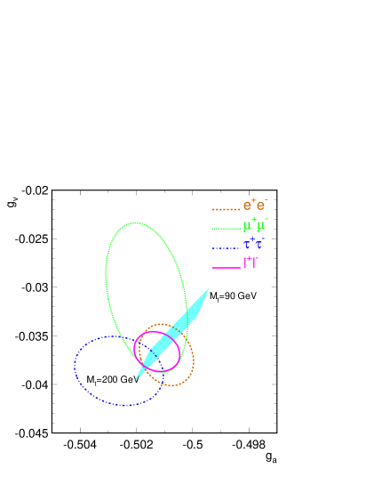
Figure 3: 68% probability contours in the $a_{l}$-$v_{l}$ plane. The solid contour assumes lepton universality. The shaded band represents the SM prediction. (Taken from Ref. [19])

Table 4 gives the averaged results obtained from the present LEP data [19]. The 68% probability contours in the $a_{l}$-$v_{l}$ plane are shown in Fig. 3. The measured ratios,

$$\!\!{v_{\mu}\over v_{e}}=0.83\pm 0.16\,,\quad{v_{\tau}\over v_{e}}=1.044\pm 0.091\,,\quad{a_{\mu}\over a_{e}}=1.0014\pm 0.0021\,,\quad{a_{\tau}\over a_{e}}=1.0034\pm 0.0023\,,$$ (10.20)

provide a test of charged-lepton universality in the neutral-current sector.

The neutrino coupling can also be determined from the invisible $Z$-decay width, by assuming three identical neutrino generations with left-handed couplings, and fixing the sign from neutrino scattering data [32]. The resulting experimental value [19],

$$v_{\nu}\,=\,a_{\nu}\,=\,-0.5011\pm 0.0018\,,$$ (10.21)

is in perfect agreement with the SM. Alternatively, one can use the SM prediction for $\Gamma_{\mbox{\rm\scriptsize inv}}$ to get a determination of the number of (light) neutrino flavours, $N_{\nu}=2.988\pm 0.023$ [19].

The measured leptonic asymmetries can be used to obtain the effective electroweak mixing angle in the charged-lepton sector [19]:

$$\sin^{2}{\theta^{\mbox{\rm\scriptsize lept}}_{\mbox{\rm\scriptsize eff}}}\,\equiv\,{1\over 4}\,\left(1-{v_{l}\over a_{l}}\right)\,=\,0.2317\pm 0.0007\,.$$ (10.22)

Since the hadronic asymmetries have a reduced sensitivity to corrections particular to the hadronic vertex, $\sin^{2}{\theta^{\mbox{\rm\scriptsize lept}}_{\mbox{\rm\scriptsize eff}}}$ can also be extracted from the quark forward-backward asymmetries. The measured values of ${\cal A}_{\mbox{\rm\scriptsize FB}}^{0,b}$ and ${\cal A}_{\mbox{\rm\scriptsize FB}}^{0,c}$ imply $\sin^{2}{\theta^{\mbox{\rm\scriptsize lept}}_{\mbox{\rm\scriptsize eff}}}=0.2325\pm 0.0006$, while the total hadronic charge asymmetry $\langle Q_{\mbox{\rm\scriptsize FB}}\rangle$ gives $0.2320\pm 0.0016$ [19]. The three LEP values are in good agreement, giving and average of $0.2321\pm 0.0004$.

A slightly smaller value,

$$\sin^{2}{\theta^{\mbox{\rm\scriptsize lept}}_{\mbox{\rm\scriptsize eff}}}\,=\,0.2294\pm 0.0010\,,$$ (10.23)

is obtained from the measurement of ${\cal A}_{\mbox{\rm\scriptsize LR}}$, performed at SLC [24]. Making a global average with the LEP determination, one gets $\sin^{2}{\theta^{\mbox{\rm\scriptsize lept}}_{\mbox{\rm\scriptsize eff}}}=0.2317\pm 0.0004$ with a $\chi^{2}/\mbox{\rm d.o.f.}=9.0/6$.

Including the full SM predictions at the 1–loop level, the $Z$ measurements can be used to obtain information on the SM parameters. Figs. 4 and 5, taken from Ref. [19], compare different LEP measurements with the corresponding SM predictions as a function of $m_{t}$. The parameters $M_{H}$ and $\alpha_{s}(M_{Z}^{2})$ have been taken in the ranges 60 GeV $<M_{H}<$ 1000 GeV and $\alpha_{s}(M_{Z}^{2})=0.123\pm 0.006$. For the comparison of $R_{b}$ with the SM the value of $R_{c}$ has been fixed to the SM prediction. The overall agreement is very good; moreover, the different observables determine a similar range of $m_{t}$. Only the ratios $R_{b}$ and $R_{c}$ seem to be slightly off.

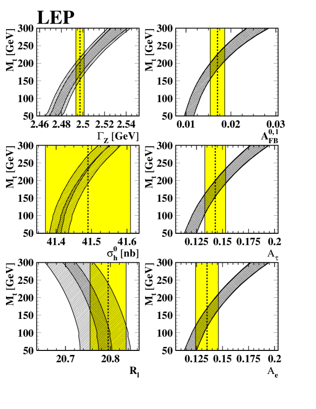
Figure 4: Comparison of LEP measurements with the SM prediction as a function of $m_{t}$. The cross-hatched area shows the variation of the SM prediction with $M_{H}$ spanning the interval 60 GeV $<M_{H}<$ 1000 GeV and the singly-hatched area corresponds to a variation of $\alpha_{s}(M_{Z}^{2})$ within the interval $\alpha_{s}(M_{Z}^{2})=0.123\pm 0.006$. The total width of the band corresponds to the linear sum of both uncertainties. The experimental errors are indicated as vertical bands. (Taken from Ref. [19]).

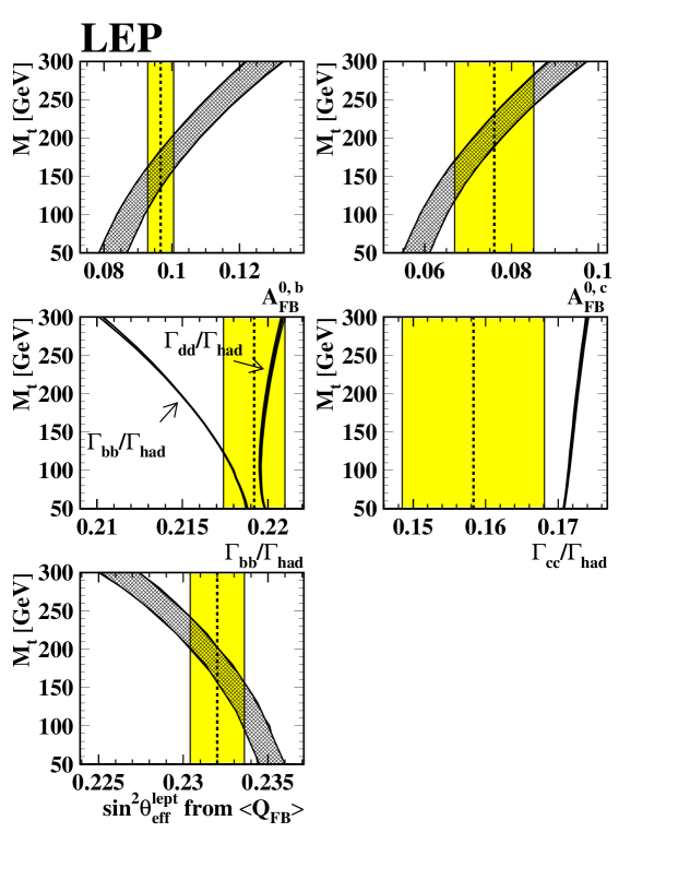
Figure 5: Same as Fig. 4.

Table 5 shows the constraints obtained on $m_{t}$ and $\alpha_{s}(M_{Z}^{2})$, from a global fit to the electroweak data [19]. The fitted value of the top mass is in perfect agreement with the CDF measurement, $m_{t}=174\pm 10{\,}^{+13}_{-12}$ GeV [23]. Moreover, the extracted value of the strong coupling agrees very well with direct determinations from event shape measurements, $\alpha_{s}(M_{Z}^{2})=0.123\pm 0.006$ [5], or $\tau$ decay, $\alpha_{s}(M_{Z}^{2})=0.119\pm 0.004$ [33].

Taking the central values for $m_{t}$ and $\alpha_{s}(M_{Z}^{2})$, the SM fit implies $R_{b}=0.2158$ and $R_{c}=0.172$. The discrepancy with the measured asymmetries $R_{b}=0.2202\pm 0.0020$ and $R_{c}=0.1583\pm 0.0098$ is at the $2.2\sigma$ and $-1.4\sigma$ level, respectively. The agreement between $R_{b}$ and its SM prediction improves to $1.9\sigma$ if $R_{c}$ is fixed to the SM value of $R_{c}=0.171$ (there is a strong correlation between both hadronic asymmetries). In this case, one obtains $R_{b}=0.2192\pm 0.0018$ [19]. Although it is still premature to extract any conclusion from this small (and statistically not significant) discrepancy, it is certainly an important thing to keep in mind, in view of the special role played by the $Z\bar{b}b$ vertex.

Since the main $M_{H}$ dependence is only logarithmic, it is not possible to extract information on $M_{H}$, without a direct measurement of $m_{t}$. If the CDF value of $m_{t}$ is used as an additional constraint on the electroweak fit, the observed $\Delta\chi^{2}\equiv\chi^{2}-\chi^{2}_{\mbox{\rm\scriptsize min}}$ curve exhibits a minimum for low values of $M_{H}$. However, at 95% CL the entire range of $M_{H}$ up to 1000 GeV is allowed.

Table 5: Values of $m_{t}$ and $\alpha_{s}(M_{Z}^{2})$ obtained from a global fit to present electroweak precision data [19]. No external constraint on $\alpha_{s}(M_{Z}^{2})$ has been imposed. The central values and the first errors quoted refer to $M_{H}=300$ GeV. The second errors correspond to the variation of the central value in the interval 60 GeV $<M_{H}<$ 1000 GeV. The bottom part of the table lists derived results for the effective leptonic electroweak mixing angle, $1-M_{W}^{2}/M_{Z}^{2}$ and $M_{W}$.

	LEP	LEP	LEP
	only	+ $p\bar{p}$ and $\nu N$ data	+ $p\bar{p}$ and $\nu N$ data + ${\cal A}_{\mbox{\rm\scriptsize LR}}$
$m_{t}$    (GeV)	$173{\,}^{+12}_{-13}{\,}^{+18}_{-20}$	$171{\,}^{+11}_{-12}{\,}^{+18}_{-19}$	$178{\,}^{+11}_{-11}{\,}^{+18}_{-19}$
$\alpha_{s}(M_{Z}^{2})$	$0.126\pm 0.005\pm 0.002$	$0.126\pm 0.005\pm 0.002$	$0.125\pm 0.005\pm 0.002$
$\chi^{2}/\mbox{\rm d.o.f.}$	$7.6/9$	$7.7/11$	$15/12$
$\sin^{2}{\theta^{\mbox{\rm\scriptsize lept}}_{\mbox{\rm\scriptsize eff}}}$	$0.2322\pm 0.0004{\,}^{+0.0001}_{-0.0002}$	$0.2323\pm 0.0003{\,}^{+0.0001}_{-0.0002}$	$0.2320\pm 0.0003{\,}^{+0.}_{-0.0002}$
$1-M_{W}^{2}/M_{Z}^{2}$	$0.2249\pm 0.0013{\,}^{+0.0003}_{-0.0002}$	$0.2250\pm 0.0013{\,}^{+0.0003}_{-0.0002}$	$0.2242\pm 0.0012{\,}^{+0.0003}_{-0.0002}$
$M_{W}$    (GeV)	$80.28\pm 0.07{\,}^{+0.01}_{-0.02}$	$80.27\pm 0.06{\,}^{+0.01}_{-0.01}$	$80.32\pm 0.06{\,}^{+0.01}_{-0.01}$

11 Quark Mixing

Our knowledge of the charged-current parameters is unfortunately not so good as in the neutral-current case. In order to measure the CKM matrix elements, one needs to study semileptonic weak decays $H\to H^{\prime}l\bar{\nu}_{l}$, associated with the corresponding quark transition $d_{j}\to u_{i}l^{-}\bar{\nu}_{l}$. Since quarks are confined within hadrons, the decay amplitude

$$T[H\to H^{\prime}l\bar{\nu}_{l}]\,\approx\,{G_{F}\over\sqrt{2}}\,\mbox{\boldmath$V$}_{\!\!ij}\,\,\langle H^{\prime}|\bar{u}_{i}\gamma^{\mu}(1-\gamma_{5})d_{j}|H\rangle\,\,\bar{l}\gamma_{\mu}(1-\gamma_{5})\nu_{l}$$ (11.1)

always involves an hadronic matrix element of the weak left current. The evaluation of this matrix element is a non-perturbative QCD problem and, therefore, introduces unavoidable theoretical uncertainties.

Usually, one looks for a semileptonic transition where the matrix element can be fixed at some kinematical point, by a symmetry principle. This has the virtue of reducing the theoretical uncertainties to the level of symmetry-breaking corrections and kinematical extrapolations. The standard example is a $0^{-}\to 0^{-}$ decay such as $K\to\pi l\nu$, $D\to Kl\nu$ or $B\to Dl\nu$. Only the vector current can contribute in this case:

$$\langle P^{\prime}(k^{\prime})|\bar{u}_{i}\gamma^{\mu}d_{j}|P(k)\rangle\,=\,C_{PP^{\prime}}\,\left\{(k+k^{\prime})^{\mu}f_{+}(t)+(k-k^{\prime})^{\mu}f_{-}(t)\right\}.$$ (11.2)

Here, $C_{PP^{\prime}}$ is a Clebsh-Gordan factor and $t=(k-k^{\prime})^{2}$. The unknown strong dynamics is fully contained in the form factors $f_{\pm}(t)$. In the massless quark limit, the divergence of the vector current is zero; thus, $f_{-}(t)=0$ and, moreover, $f_{+}(0)=1$ because the associated flavour charge is a conserved quantity. Therefore, one only needs to estimate the corrections induced by the finite values of the quark masses.

Since $(k-k^{\prime})^{\mu}\,\bar{l}\gamma_{\mu}(1-\gamma_{5})\nu_{l}\sim m_{l}$, the contribution of $f_{-}(t)$ is kinematically suppressed in the $e$ and $\mu$ modes. The decay width can then be written as

$$\Gamma(P\to P^{\prime}l\nu)\,=\,{G_{F}^{2}M_{P}^{5}\over 192\pi^{3}}\,|\mbox{\boldmath$V$}_{\!\!ij}|^{2}\,C_{PP^{\prime}}^{2}\,|f_{+}(0)|^{2}\,{\cal I}\,\left(1+\delta_{\mbox{\rm\scriptsize RC}}\right),$$ (11.3)

where $\delta_{\mbox{\rm\scriptsize RC}}$ is an electroweak radiative correction factor and ${\cal I}$ denotes a phase-space integral, which in the $m_{l}=0$ limit takes the form

$${\cal I}\,\approx\,\int_{0}^{(M_{P}-M_{P^{\prime}})^{2}}{dt\over M_{P}^{8}}\,\lambda^{3/2}(t,M_{P}^{2},M_{P^{\prime}}^{2})\,\left|{f_{+}(t)\over f_{+}(0)}\right|^{2}.$$ (11.4)

The usual procedure to determine $|\mbox{\boldmath$V$}_{\!\!ij}|$ involves three steps:

1. Measure the shape of the $t$ distribution. This fixes the ratio $|f_{+}(t)/f_{+}(0)|$ and therefore determines ${\cal I}$.

2. Measure the total decay width $\Gamma$. Since $G_{F}$ is already known from $\mu$ decay, one gets then an experimental value for the product $|f_{+}(0)|\,|\mbox{\boldmath$V$}_{\!\!ij}|$.

3. Get a theoretical prediction for $f_{+}(0)$.

The important point to realize is that theoretical input is always needed. Thus, the accuracy of the $|\mbox{\boldmath$V$}_{\!\!ij}|$ determination is limited by our ability to calculate the relevant hadronic input.

11.1 V${}_{\!ud}$

The most accurate measurement of $\mbox{\boldmath$V$}_{\!\!ud}$ is done with superallowed nuclear $\beta$ decays of the Fermi type [$0^{+}\to 0^{+}$], where the nuclear matrix element $\langle N^{\prime}|\bar{u}\gamma^{\mu}d|N\rangle$ can be fixed by vector-current conservation. The CKM factor is obtained through the relation [34],

$$|\mbox{\boldmath$V$}_{\!\!ud}|^{2}\,=\,{\pi^{3}\ln{2}\over ft\,G_{F}^{2}m_{e}^{5}\,(1+\delta_{\mbox{\rm\scriptsize RC}})}\,=\,{(2984.4\pm 0.1)\,\mbox{\rm s}\over ft\,(1+\delta_{\mbox{\rm\scriptsize RC}})},$$ (11.5)

where the factor $ft$ denotes a “comparative half-life” corrected for phase-space and Coulomb effects [35]. In order to obtain $|\mbox{\boldmath$V$}_{\!\!ud}|$, one needs to perform a careful analysis of radiative corrections [36], including both short-distance contributions $\Delta_{\mbox{\rm\scriptsize inner}}=0.0234\pm 0.0012$, and nucleus-dependent corrections $\Delta_{\mbox{\rm\scriptsize outer}}\equiv\delta_{\mbox{\rm\scriptsize RC}}-\Delta_{\mbox{\rm\scriptsize inner}}$. These radiative corrections are quite large, $\delta_{\mbox{\rm\scriptsize RC}}\sim 3$-4%, and have a crucial role in order to bring the results from different nuclei into good agreement. The final result quoted by the Particle Data Group [8] is

$$|\mbox{\boldmath$V$}_{\!\!ud}|\,=\,0.9744\pm 0.0010\,.$$ (11.6)

An independent determination can be obtained from neutron decay, $n\to pe^{-}\nu_{e}$. The axial current also contributes in this case; therefore, one needs the experimental determination of the axial coupling $g_{A}=1.2573\pm 0.0028$ [8]. The measured neutron lifetime, $\tau_{n}=887.0\pm 2.0$ s, implies [34]:

$$|\mbox{\boldmath$V$}_{\!\!ud}|\,=\,\left\{{(4904.0\pm 5.0)\,\mbox{\rm s}\over\tau_{n}(1+3g_{A}^{2})}\right\}^{1/2}\,=\,0.981\pm 0.002\,,$$ (11.7)

which is bigger than (11.6). Thus, a better measurement of $g_{A}$ and $\tau_{n}$ is needed.

The pion $\beta$-decay $\pi^{+}\to\pi^{0}e^{+}\nu_{e}$ offers a cleaner way to measure $|\mbox{\boldmath$V$}_{\!\!ud}|$. It is a pure vector transition, with very small theoretical uncertainties. Unfortunately, owing to the kinematical suppression, it has a small branching fraction. The present experimental value is not very precise, Br=$(1.025\pm 0.034)\times 10^{-8}$; it implies $|\mbox{\boldmath$V$}_{\!\!ud}|=0.968\pm 0.018$. An accurate measurement of this transition would be very valuable.

11.2 V${}_{\!us}$

The decays $K^{+}\to\pi^{0}l^{+}\nu_{l}$ and $K^{0}\to\pi^{-}l^{+}\nu_{l}$ are ideal for measuring $|\mbox{\boldmath$V$}_{\!\!us}|$, because the relevant hadronic form factors are well understood. $SU(3)$ breaking corrections are very suppressed [37] and isospin violations can be easily taken into account: $f_{+}^{K^{0}\pi^{-}}(0)=1+{\cal O}[(m_{s}-m_{u})^{2}]$; $f_{+}^{K^{+}\pi^{0}}(0)=1+3(m_{d}-m_{u})/(4m_{s}-2m_{u}-2m_{d})+\ldots$ Moreover, higher-order corrections have been estimated [38], using Chiral Perturbation Theory methods [38, 39]. The resulting values [38], $f_{+}^{K^{0}\pi^{-}}(0)=0.977$ and $f_{+}^{K^{+}\pi^{0}}(0)/f_{+}^{K^{0}\pi^{-}}(0)=1.022$, should be compared with the experimental ratio [8] $|f_{+}^{K^{+}\pi^{0}}(0)/f_{+}^{K^{0}\pi^{-}}(0)|=1.028\pm 0.010$. The accurate calculation of these quantities allows to extract [40] a precise determination of $|\mbox{\boldmath$V$}_{\!\!us}|$:

$$|\mbox{\boldmath$V$}_{\!\!us}|\,=\,0.2196\pm 0.0023\,.$$ (11.8)

The analysis of semileptonic hyperon decay data can also provide information on $|\mbox{\boldmath$V$}_{\!\!us}|$. However, the theoretical uncertainties are much larger, owing to the first-order $SU(3)$-breaking effects in the axial-vector couplings [41]. The Particle Data Group [8] quotes the result $|\mbox{\boldmath$V$}_{\!\!us}|\,=\,0.222\pm 0.003$. The average with (11.8) gives the final value:

$$|\mbox{\boldmath$V$}_{\!\!us}|\,=\,0.2205\pm 0.0018\,.$$ (11.9)

11.3 V${}_{\!cd}$ and V${}_{\!cs}$

The value of $|\mbox{\boldmath$V$}_{\!\!cd}|$ is deduced from deep inelastic $\nu_{\mu}$ and $\bar{\nu}_{\mu}$ scattering data, by measuring the dimuon production rates off valence $d$ quarks; i.e. $\nu_{\mu}d\to\mu^{-}c$ with the charm quark detected through $c\to\mu^{+}\nu_{\mu}d$ or $\mu^{+}\nu_{\mu}s$. One gets in this way, the product [8] $\overline{B}_{c}\,|\mbox{\boldmath$V$}_{\!\!cd}|^{2}=(0.47\pm 0.05)\times 10^{-2}$, where $\overline{B}_{c}$ is the average semileptonic branching fraction of the produced charmed hadrons. Using $\overline{B}_{c}=0.113\pm 0.015$ [8], yields

$$|\mbox{\boldmath$V$}_{\!\!cd}|\,=\,0.204\pm 0.017\,.$$ (11.10)

Similarly, one could extract $|\mbox{\boldmath$V$}_{\!\!cs}|$ from $\nu_{\mu}s\to\mu^{-}c$ data. The resulting values depend, however, on assumptions about the strange quark density in the parton-sea. Making the conservative assumption that the strange quark-sea does not exceed the value corresponding to an $SU(3)$ symmetric sea, leads to the lower bound [42] $|\mbox{\boldmath$V$}_{\!\!cs}|>0.59$.

Better information is obtained from the decay $D\to\bar{K}e^{+}\nu_{e}$. The measured $t$ distribution [8] can be fitted with the parametrization $f_{+}^{D}(t)/f_{+}^{D}(0)=M^{2}/(M^{2}-t)$ and $M=2.1$ GeV; this determines the corresponding integral ${\cal I}$. Using $\Gamma(D\to\bar{K}e^{+}\nu_{e})=(0.762\pm 0.055)\times 10^{11}$ s^-1, one gets [8]:

$$|f_{+}^{D}(0)|\,|\mbox{\boldmath$V$}_{\!\!cs}|\,=\,0.704\pm 0.026\,.$$ (11.11)

The status of our theoretical understanding of charm form factors is quite crude. The symmetry arguments are not very helpful here, because the charm-quark mass is too heavy for using the $SU(4)$ massless limit, and, at the same time, is too light to believe the naive results obtained in the limit $m_{c}\to\infty$. Symmetry-breaking corrections are very important. The conservative assumption $|f_{+}^{D}(0)|<1$, implies $|\mbox{\boldmath$V$}_{\!\!cs}|>0.62$. The Particle Data Group [8] takes the range $|f_{+}^{D}(0)|=0.7\pm 0.1$, which covers the main part of the existing calculations, and quotes:

$$|\mbox{\boldmath$V$}_{\!\!cs}|\,=\,1.01\pm 0.18\,.$$ (11.12)

Theoretical uncertainties are largely avoided by taking ratios, such as $\Gamma(D\to\pi l\nu_{l})/\Gamma(D\to\bar{K}l\nu_{l})$, where the form-factor uncertainty is reduced to the level of $SU(3)$ breaking. The present measurements of the $D\to\pi l\nu_{l}$ decays are still too poor to be competitive. However, a 1% measurement of these semileptonic ratios seems possible at a future tau-charm factory; this would allow a precise determination of $|\mbox{\boldmath$V$}_{\!\!cd}|/|\mbox{\boldmath$V$}_{\!\!cs}|$.

11.4 V${}_{\!cb}$ and V${}_{\!ub}$

Assuming that the inclusive semileptonic decay width of a bottom hadron is given by the corresponding quark decay $b\to cl\nu_{l}$, the magnitude of $|\mbox{\boldmath$V$}_{\!\!cb}|$ can be determined from the ratio of the measured semileptonic branching ratio and lifetime. However, since $\Gamma(b\to cl\nu_{l})\propto m_{b}^{5}$, this method is very sensitive to the not so well-known value of the $b$-quark mass. Moreover, higher-order QCD corrections are sizeable. A recent experimental summary [43] quotes the results: $|\mbox{\boldmath$V$}_{\!\!cb}|=0.039\pm 0.001\pm 0.005$ from $\Upsilon(4S)$ data, and $|\mbox{\boldmath$V$}_{\!\!cb}|=0.042\pm 0.002\pm 0.005$ from LEP data, where the second error gives an educated guess of the theoretical uncertainty.

The cleanest determination of $|\mbox{\boldmath$V$}_{\!\!cb}|$ uses the decay $B\to D^{*}l\bar{\nu}_{l}$ [44], where the relevant hadronic form factor [${\cal F}(v_{B}\cdot v_{D^{*}})$] can be controlled at the level of a few per cent, close to the zero-recoil region. In the infinite $B$-mass limit, the normalization of this form factor at zero recoil is fixed to be one, and the leading $1/M$ corrections vanish [45] due to heavy-quark symmetry; thus the theoretical uncertainty is of order $1/M^{2}$ and therefore in principle small. The calculated short-distance QCD corrections and the present estimates of the $1/M^{2}$ contributions result in ${\cal F}(1)=0.93\pm 0.03$ [46], implying

$$|\mbox{\boldmath$V$}_{\!\!cb}|=0.040\pm 0.003\,.$$ (11.13)

The present determination of $|\mbox{\boldmath$V$}_{\!\!ub}|$ is based on measurements of the lepton momentum spectrum in inclusive $B\to X_{q}l\bar{\nu}_{l}$ decays, where $X_{q}$ is any hadronic state containing a quark $q=c$ or $u$. The method is very sensitive to the assumed theoretical spectrum near the kinematic limit for $B\to Dl\bar{\nu}_{l}$. Using different models to estimate the systematic theoretical uncertainties, the analyses of the experimental data give [8]

$$\left|{\mbox{\boldmath$V$}_{\!\!ub}/\mbox{\boldmath$V$}_{\!\!cb}}\right|\,=\,0.08\pm 0.02\,.$$ (11.14)

Eq. (11.13), implies then $|\mbox{\boldmath$V$}_{\!\!ub}|=0.003\pm 0.001$.

11.5 Unitarity

The present status of direct $\mbox{\boldmath$V$}_{\!\!ij}$ determinations can be easily summarized:

• The light-quark mixings $|\mbox{\boldmath$V$}_{\!\!ud}|$ and $|\mbox{\boldmath$V$}_{\!\!us}|$ are rather well-known (0.1% and 0.8% accuracy, respectively). Moreover, since the theory is good, improved values could be obtained with better data on semileptonic $\pi^{+}$ and $K$ decays.

• $|\mbox{\boldmath$V$}_{\!\!cd}|$ and $|\mbox{\boldmath$V$}_{\!\!cs}|$ are very badly known (8% and 18% accuracy, respectively). This could be largely improved at a tau-charm factory. Much better theoretical input is needed.

• $|\mbox{\boldmath$V$}_{\!\!cb}|$ and $|\mbox{\boldmath$V$}_{\!\!ub}|$ are also badly known (8% and 33% accuracy, respectively). However, there are good theoretical tools available. Thus, better determinations could be easily performed at a $B$ factory.

• Nothing is known about the CKM mixings involving the top quark.

The entries of the first row are already accurate enough to perform a sensible test of the unitarity of the CKM matrix:

$$|\mbox{\boldmath$V$}_{\!\!ud}|^{2}+|\mbox{\boldmath$V$}_{\!\!us}|^{2}+|\mbox{\boldmath$V$}_{\!\!ub}|^{2}\,=\,0.9981\pm 0.0027\,.$$ (11.15)

It is important to notice that radiative corrections play here a crucial role. If one uses $|\mbox{\boldmath$V$}_{\!\!uj}|$ values determined without radiative corrections, the result (11.15) changes to $1.0384\pm 0.0027$, giving an apparent violation of unitarity (by many $\sigma$’s) [34].

Imposing the unitarity constraint $\mbox{\boldmath$V$}\mbox{\boldmath$V$}^{\dagger}=\mbox{\boldmath$V$}^{\dagger}\mbox{\boldmath$V$}=1$ (and assuming only three generations) one can get a more precise picture of the CKM matrix. The 90% confidence limits on the magnitude of the CKM matrix elements are then [8]:

$$\mbox{\boldmath$V$}\,=\,\left[\begin{array}[]{ccc}0.9747\,\,\mbox{\rm to}\,\,0.9759&0.218\,\,\mbox{\rm to}\,\,0.224&0.002\,\,\mbox{\rm to}\,\,0.005\\ 0.218\,\,\mbox{\rm to}\,\,0.224&0.9738\,\,\mbox{\rm to}\,\,0.9752&0.032\,\,\mbox{\rm to}\,\,0.048\\ 0.004\,\,\mbox{\rm to}\,\,0.015&0.030\,\,\mbox{\rm to}\,\,0.048&0.9988\,\,\mbox{\rm to}\,\,0.9995\end{array}\right].$$ (11.16)

The ranges given here are slightly different from (but consistent with) the direct determinations mentioned before.

The resulting CKM matrix shows a hierarchical pattern, with the diagonal elements being very close to one, the ones connecting the two first generations having a size $\lambda\equiv|\mbox{\boldmath$V$}_{\!\!us}|=0.2205\pm 0.0018$, the mixing between the second and third families being of order $\lambda^{2}$, and the mixing between the first and third quark flavours having a much smaller size of about $\lambda^{3}$. It is then quite practical to use the approximate parametrization [47]:

$$\mbox{\boldmath$V$}\,=\,\left[\matrix{\displaystyle\ 1-{\lambda^{2}\over 2}\hfill&\displaystyle\ \ \ \ \ \ \lambda\hfill&\displaystyle\ \ \ \ \ A\lambda^{3}(\rho-i\eta)\hfill\cr\displaystyle\hfill&\displaystyle\hfill&\displaystyle\hfill\cr\displaystyle\ \ \ -\lambda\hfill&\displaystyle\ \ \ \ \ 1-{\lambda^{2}\over 2}\hfill&\displaystyle\ \ \ \ \ A\lambda^{2}\hfill\cr\displaystyle\hfill&\displaystyle\hfill&\displaystyle\hfill\cr\displaystyle\ A\lambda^{3}(1-\rho-i\eta)\hfill&\displaystyle\ \ \ \ \ -A\lambda^{2}\hfill&\displaystyle\ \ \ \ \ \ \ \ \ 1\hfill\cr}\right]\ +\ O\left(\lambda^{4}\right)\,,$$ (11.17)

where $A=|\mbox{\boldmath$V$}_{\!\!cb}|/\lambda^{2}=0.82\pm 0.06$, and

$$\sqrt{\rho^{2}+\eta^{2}}\,=\,\left|{\mbox{\boldmath$V$}_{\!\!ub}\over\lambda\mbox{\boldmath$V$}_{\!\!cb}}\right|\,=\,0.36\pm 0.09\,.$$ (11.18)

11.6 Indirect determinations

Additional information can be obtained from flavour-changing neutral-current transitions, occurring at the 1–loop level. An important example is provided by the mixing between the $B^{0}$ meson and its antiparticle. This process occurs through the exchange of two $W$’s between the fermionic lines, the so-called box diagrams. The mixing amplitude is proportional to

$$\langle\bar{B}_{d}^{0}|{\cal H}|B_{0}\rangle\,\sim\,\sum_{ij}\,\mbox{\boldmath$V$}_{\!\!id}^{\phantom{*}}\mbox{\boldmath$V$}_{\!\!ib}^{*}\mbox{\boldmath$V$}_{\!\!jd}^{*}\mbox{\boldmath$V$}_{\!\!jb}^{\phantom{*}}\,S(r_{i},r_{j}),$$ (11.19)

where $S(r_{i},r_{j})$ is a loop function which depends on the masses [$r_{i}\equiv m_{i}^{2}/M_{W}^{2}$] of the up-type quarks running along the internal lines. Owing to the unitarity of the CKM matrix, the mixing amplitude vanishes for equal (up-type) quark masses (GIM mechanism); thus the effect is proportional to the mass splittings between the $u$, $c$ and $t$ quarks. Since the different CKM factors have all a similar size, $\mbox{\boldmath$V$}_{\!\!ud}^{\phantom{*}}\mbox{\boldmath$V$}_{\!\!ub}^{*}\sim\mbox{\boldmath$V$}_{\!\!cd}^{\phantom{*}}\mbox{\boldmath$V$}_{\!\!cb}^{*}\sim\mbox{\boldmath$V$}_{\!\!td}^{\phantom{*}}\mbox{\boldmath$V$}_{\!\!tb}^{*}\sim A\lambda^{3}$, the final amplitude is completely dominated by the top contribution; i.e. $\langle\bar{B}_{d}^{0}|{\cal H}|B_{0}\rangle\,\sim\,|\mbox{\boldmath$V$}_{\!\!tb}|^{2}S(r_{t},r_{t})$.

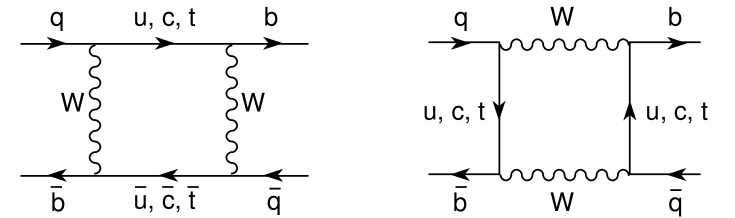
Figure 6: $B^{0}$-$\bar{B}^{0}$ mixing diagrams.

One can then determine $|\mbox{\boldmath$V$}_{\!\!td}|$ from the measured mixing $x_{d}\equiv\Delta M_{B_{d}}/\Gamma_{B_{d}}=0.76\pm 0.06$ [48]. Unfortunately, one also needs to know the hadronic matrix element of the 4-quark operator $(\bar{b}_{L}\gamma^{\mu}d_{L})(\bar{b}_{L}\gamma_{\mu}d_{L})$ between the $B^{0}$ and $\bar{B}^{0}$ states. This is again a non-perturbative QCD problem, which introduces a big theoretical uncertainty. The most recent analysis [49] gets:

$$|\mbox{\boldmath$V$}_{\!\!td}|\,=\,0.007{\,}^{+0.003}_{-0.002}\,,$$ (11.20)

in good agreement with (but more precise than) the value obtained from the unitarity constraint in Eq. (11.16). In terms of the $(\rho,\eta)$ parametrization of Eq. (11.17), this gives

$$\sqrt{(1-\rho)^{2}+\eta^{2}}\,=\,\left|{\mbox{\boldmath$V$}_{\!\!td}\over\lambda\mbox{\boldmath$V$}_{\!\!cb}}\right|\,=\,0.8{\,}^{+0.3}_{-0.2}\,.$$ (11.21)

Notice that together with (11.18), this result implies $\eta\not=0$; although errors are still too large to make any strong statement. Thus, if CKM unitarity is assumed, it is possible to establish the existence of CP violation from CP conserving measurements. A more direct constraint on the parameter $\eta$ is provided [49] by the measured CP violation in the $K^{0}$-$\bar{K}^{0}$ system, $\varepsilon_{K}$.

12 Charged-Current Lepton Universality

In the SM, the $W$ couples with the same strength $g/(2\sqrt{2})$ to all charged fermionic currents (up to CKM mixing factors in the quark sector). The universality of the leptonic couplings can be easily tested, by allowing these couplings to depend on the considered lepton flavour and comparing several leptonic and semileptonic decays.

The ratio $R_{e/\mu}$ of the two semileptonic $\pi^{-}\to l^{-}\bar{\nu}_{l}$ decay modes is proportional to $|g_{e}/g_{\mu}|^{2}$. From Eq. (2.8), one inmediately gets:

$$\left|{g_{\mu}/g_{e}}\right|\,=\,1.0021\pm 0.0016\,.$$ (12.1)

A less accurate value, $\left|g_{\mu}/g_{e}\right|=1.004\pm 0.009$, is obtained from the ratio $B_{\tau\to\mu}/B_{\tau\to e}=0.9800\pm 0.017$ [8], where $B_{\tau\to l}\equiv\Gamma(\tau^{-}\to l^{-}\bar{\nu}_{l}\nu_{\tau})$.

Comparing $\Gamma(\tau^{-}\to e^{-}\bar{\nu}_{e}\nu_{\tau})$ and $\Gamma(\mu^{-}\to e^{-}\bar{\nu}_{e}\nu_{\mu})$ [see Eq. (2.3)], one can test $g_{\tau}$:

$$\left|{g_{\tau}\over g_{\mu}}\right|\,=\,\left\{B_{\tau\to e}\,{\tau_{\mu}m_{\mu}^{5}\,f(m_{e}^{2}/m_{\mu}^{2})\,(1+\delta^{\mu}_{\mbox{\rm\scriptsize RC}})\over\tau_{\tau}m_{\tau}^{5}\,f(m_{e}^{2}/m_{\tau}^{2})\,(1+\delta^{\tau}_{\mbox{\rm\scriptsize RC}})}\right\}^{1/2}\,=\,0.997\pm 0.007\,.$$ (12.2)

Other (less precise) tests of lepton universality are obtained from $p\bar{p}$ collider data on leptonic $W$ decays, and from the ratio of the $\Gamma[\tau^{-}\to\nu_{\tau}\pi^{-}(K^{-})]$ and $\Gamma[\pi^{-}(K^{-})\to l^{-}\bar{\nu}_{l}]$ decay widths [50].

The $V-A$ structure of the $\tau$ charged current can also be studied, following the same kind of analysis performed for $\mu$ decay (see Sect. 2.1). Unfortunately, the data is still not accurate enough to determine the interaction. Assuming that the $\tau\nu_{\tau}W$ vertex is a linear combination of vector and axial currents, $g_{V}^{(\tau)}V^{\mu}-g_{A}^{(\tau)}A^{\mu}$, and using the SM $V-A$ form for the other $W$ couplings, one gets the constraints [50, 51]:

$$\left|{g_{V}^{(\tau)}-g_{A}^{(\tau)}\over g_{V}^{(\tau)}+g_{A}^{(\tau)}}\right|\,<\,0.37\qquad(95\%\mbox{\rm CL}),\qquad\qquad{2g_{V}^{(\tau)}g_{A}^{(\tau)}\over\left|g_{V}^{(\tau)}\right|^{2}+\left|g_{A}^{(\tau)}\right|^{2}}\,=\,1.022\pm 0.041.$$ (12.3)

13 Summary and Outlook

The SM provides a beautiful theoretical framework which is able to accommodate all our present knowledge on electroweak interactions. It is able to explain any single experimental fact, and in some cases, such as the neutral-current sector, has succesfully passed very precise tests at the 0.1% to 1% level. However, there are still pieces of the SM Lagrangian which so-far have not been experimentally analyzed in any precise way. Moreover, the SM leaves many unaswered questions and contains too many free parameters to qualify as an ultimate fundamental theory. Clearly, new physics should exist.

The discovery of the top quark [23] is awaiting confirmation. In addition to complete the SM fermionic structure in the third generation, an accurate measurement of $m_{t}$ is needed to improve the significance of present neutral-current analyses at the $Z$ peak. Together with a much better meaurement of $\Gamma(Z\to\bar{b}b)$, that would provide a non-trivial consistency test of the SM at the quantum level, including effects related with the longitudinal gauge-boson polarization.

The gauge self-couplings will be investigated at LEP II, through the study of the $e^{+}e^{-}\to W^{+}W^{-}$ production cross-section. The $V-A$ ($\nu_{e}$-exchange in the $t$ channel) contribution generates an unphysical growing of the cross-section with the centre-of-mass energy, which is compensated through a delicate gauge cancellation with the $e^{+}e^{-}\to\gamma,Z\to W^{+}W^{-}$ amplitudes. This offers a good way to test the gauge-boson self-interactions. The study of this process will also provide a more accurate measurement of $M_{W}$, allowing to improve the precision of present LEP I analyses.

The Higgs particle is the main missing block of the SM framework. The present experimental lower bound is [8]

$$M_{H}\,>\,58.4\,\,\mbox{\rm GeV}\qquad\qquad(95\%\,\mbox{\rm CL}).$$ (13.1)

LEP II first and later LHC will try to find out wether such scalar field exists. Note that the present succesful tests of the $\rho_{0}=1$ prediction only provide a confirmation of the assumed pattern of SSB, but do not prove the minimal Higgs mechanism embedded in the SM.

The Higgs width increases very fast with its mass [$\Gamma(H\to W^{+}W^{-},ZZ)\sim G_{F}M_{H}^{3}$]. At $M_{H}\sim 1$ TeV, $\Gamma_{H}\sim M_{H}$; thus a heavy Higgs would look experimentally like a very broad resonant structure rather than as a “fundamental” peak. In fact, since the $|\phi|^{4}$ coupling grows with $M_{H}$ ($h\sim M_{H}^{2}$), at such large masses the Higgs interactions are very strong. For $M_{H}\geq\sqrt{2}v\approx 348$ GeV, $h\geq 1$ and the SM enters into a non-perturbative strong-coupling regime. A naive resummation of higher-order corrections to the $|\phi|^{4}$ vertex generates an effective “running” coupling $h(s)$, which grows with the energy scale and blows up (Landau pole) at $\sqrt{s}\sim v\exp{\left\{-3M_{H}^{2}/(4\pi^{2}v^{2})\right\}}$. The perturbative predictions become completely meaningless above $s\sim M_{H}\sim 815$ GeV. A similar phenomenon happens in the scattering of longitudinal gauge bosons, where the tree-level $W^{+}_{L}W^{-}_{L}\to W^{+}_{L}W^{-}_{L}$ amplitude violates the unitarity limit for $M_{H}\geq 713$ GeV; higher-order contributions (which obviously would restore unitarity) are then huge, indicating again a non-perturbative regime. Thus, the experimental investigation of the SSB mechanism at higher-energy machines could provide hints of completely new phenomena.

The family structure and the pattern of fermionic masses and mixings constitute a “terra incognita”, where we know nothing else than the empirical determinations of the relevant parameters. Flavour factories (such as kaon, tau-charm, $B$ or even a futuristic top factory) are needed in order to make an accurate investigation of the properties of the different fermionic flavours. A precise (and overconstrained) measurement of the quark-mixing parameters would allow to test the unitarity structure of the CKM matrix.

CP-violation offers an interesting window into possible new physics. The tiny violation of the CP symmetry observed in the kaon system, can be parametrized through the CKM phase. However, a fundamental explanation of the origin of this phenomena is lacking. In the SM, all CP-violating effects should be explained by a single parameter $\delta_{13}$; moreover, any signal should disappear in the limit where any two equal-charge quarks become degenerate in mass (the CP phase could then be rotated away by a field redefinition). Thus, the SM makes very precise predictions for CP-violating observables, which should be tested in appropriate experiments.

Finally, the possibility of non-zero neutrino massess, and the associated lepton-flavour violation phenomena, should be investigated. Moreover, a better knowledge of the $\tau$-neutrino properties is required. The existence of the $\nu_{\tau}$ as a different neutrino flavour can be inferred from the measured invisible $Z$ width; however, so far, nobody has been able to detect a single $\nu_{\tau}$ interaction.

Clearly, we need more experiments in order to learn what kind of physics exists beyond the present SM frontiers. We have, fortunately, a very promising and exciting future ahead of us.

References

References

• [1] S.L. Glashow, Nucl. Phys. 22 (1961) 579.
• [2] S. Weinberg, Phys. Rev. Lett. 19 (1967) 1264.
• [3] A. Salam, in Elementary Particle Theory, ed. N. Svartholm (Almquist and Wiksells, Stockholm, 1969), p. 367.
• [4] S.L. Glashow, J. Iliopoulos and L. Maiani, Phys. Rev. D2 (1970) 1285.
• [5] D. Espriu, Perturbative QCD, these proceedings;
A. Pich, Quantum ChromoDynamics, lectures given at the 1994 CERN-JINR Summer School (Sorrento, Italy, September 1994).
• [6] W. Fetscher, H.-J. Gerber and K.F. Johnson, Phys. Lett. B173 (1986) 102.
• [7] T. Kinoshita and A. Sirlin, Phys. Rev. 113 (1959) 1652.
• [8] Particle Data Group, Review of Particle Properties, Phys. Rev. D50 (1994) 1173.
• [9] W.J. Marciano and A. Sirlin, Phys. Rev. Lett. 71 (1993) 3629.
• [10] G. Danby et al., Phys. Rev. Lett. 9 (1962) 36.
• [11] N. Cabibbo, Phys. Rev. Lett. 10 (1963) 531.
• [12] T.D. Lee and C.N. Yang, Phys. Rev. Lett. 4 (1960) 307.
• [13] H.J. Hasert et al., Phys. Lett. 46B (1973) 121.
• [14] T. Kinoshita (editor), Quantum Electrodynamics, Advanced Series on Directions in High Energy Physics, Vol. 7 (World Scientific, Singapore, 1990);
T. Kinoshita, Phys. Rev. D47 (1993) 5013.
• [15] J. Goldstone, Nuov. Cim. 19 (1961) 154.
• [16] P.W. Higgs, Phys. Rev. 145 (1966) 1156;
T.W.B Kibble, Phys. Rev. 155 (1967) 1554.
• [17] G. ’t Hooft, Nucl. Phys. B33 (1971) 173.
• [18] G. Arnison et al. (UA1), Phys. Lett. B122 (1983) 103; B126 (1993) 398;
M. Banner et al. (UA2), Phys. Lett. B122 (1983) 476; B129 (1983) 130.
• [19] The LEP Collaborations and the LEP Electroweak Working Group, CERN/PPE/94-187.
• [20] M. Demarteau et al., CDF/PHYS/CDF/PUBLIC/2552 and D0 NOTE 2115.
• [21] J.J. Aubert et al., Phys. Rev. Lett. 33 (1974) 1404;
J.E. Augustin et al., Phys. Rev. Lett. 33 (1974) 1406; 1453.
• [22] M. Kobayashi and T. Maskawa, Prog. Theor. Phys. 42 (1973) 652.
• [23] F. Abe et al (CDF), Phys. Rev. D50 (1994) 2966; Phys. Rev. Lett. 73 (1994) 225.
• [24] K. Abe et al. (SLD), Phys. Rev. Lett. 73 (1994) 25.
• [25] H. Burkhardt et al., Z. Phys. C43 (1989) 497.
• [26] M. Veltman, Nucl. Phys. B123 (1977) 89.
• [27] J. Bernabéu, A. Pich and A. Santamaría, Phys. Lett. B200 (1988) 569; Nucl. Phys. B363 (1991) 326.
• [28] A. Sirlin, Phys. Rev. D22 (1980) 971.
• [29] T. Appelquist and J. Carazzone, Phys. Rev. D11 (1975) 2856.
• [30] A.A. Akhundov, D. Yu. Bardin and T. Riemann, Nucl. Phys. B276 (1986) 1;
W. Beenakker and W. Hollik, Z. Phys. C40 (1988) 141;
B.W. Lynn and R.G. Stuart, Phys. Lett. B252 (1990) 676.
• [31] J.M. Benlloch et al., Z. Phys. C59 (1993) 471.
• [32] P. Vilain et al. (CHARM II), Phys. Lett. B335 (1994) 246.
• [33] A. Pich, QCD Predictions for the $\tau$ Hadronic Width: Determination of $\alpha_{s}(M_{\tau}^{2})$, to appear in Proc. QCD 94 Workshop (Montpellier, 1994) [Valencia preprint FTUV/94-71].
• [34] W.J. Marciano, Annu. Rev. Nucl. Part. Sci. 41 (1991) 469.
• [35] J.C. Hardy et al., Nucl. Phys. A509 (1990) 429.
• [36] W.J. Marciano and A. Sirlin, Phys. Rev. Lett. 56 (1986) 22;
A. Sirlin and R. Zucchini, Phys. Rev. Lett. 57 (1986) 1994;
A. Sirlin, Phys. Rev. D35 (1987) 3423;
W. Jaus and G. Rasche, Phys. Rev. D35 (1987) 3420; D41 (1990) 166.
• [37] M. Ademollo and R. Gatto, Phys. Rev. Lett. 13 (1964) 264.
• [38] J. Gasser and H. Leutwyler, Nucl. Phys. B250 (1985) 465; 517; 539.
• [39] A. Pich, Introduction to Chiral Perturbation Theory, Proc. Fifth Mexican School of Particles and Fields (Guanajuato, Mexico, 1992), eds. J.L. Lucio M. and M. Vargas, AIP Conference Proceedings 317 (New York, 1994), p. 95.
• [40] H. Leutwyler and M. Roos, Z. Phys. C25 (1984) 91.
• [41] J.F. Donoghue, B.R. Holstein and S.W. Klimt, Phys. Rev. D35 (1987) 934.
• [42] H. Abramowicz et al., Z. Phys. C15 (1982) 19.
• [43] R. Patterson, Weak and rare decays, to appear in Proc. of the 27th Int. Conf. on High Energy Physics (Glasgow, 1994).
• [44] M. Neubert, Phys. Lett. B264 (1991) 455.
• [45] M. Luke, Phys. Lett. B252 (1990) 447.
• [46] M. Neubert, Phys. Lett. B338 (1994) 84.
• [47] L. Wolfenstein, Phys. Rev. Lett. 51 (1983) 1945.
• [48] R. Forty, CP Violation and $B^{0}$-$\bar{B}^{0}$ Mixing, to appear in Proc. of the 27th Int. Conf. on High Energy Physics (Glasgow, 1994).
• [49] A. Pich and J. Prades, Valencia preprint FTUV/94-37.
• [50] A. Pich, Nucl. Phys. B (Proc. Suppl.) 31 (1993) 213.
• [51] H. Albrecht et al. (ARGUS), Phys. Lett. B337 (1994) 383.
• [52] J. Bernabéu and P. Pascual, Electro-Weak Theory, GIFT report (University Autónoma of Barcelona, Bellaterra, 1981).