FTUV/94-71 IFIC/94-68 hep-ph/9412273 November 1994 QCD Predictions for the $\tau$ Hadronic Width: Determination of $\alpha_{s}(M_{\tau}^{2})$

Abstract

The total $\tau$ hadronic width can be accurately calculated using analyticity and the operator product expansion. The theoretical analysis of this observable is updated to include all available perturbative and non-perturbative corrections. The experimental determination of $\alpha_{s}(M_{\tau}^{2})$ and its actual uncertainties are discussed.

1 INTRODUCTION

The inclusive character of the total $\tau$ hadronic width renders possible an accurate calculation of the ratio [1, 2, 3, 4, 5, 6, 7]

$$R_{\tau}\equiv{\Gamma[\tau^{-}\rightarrow\nu_{\tau}\,\mbox{\rm hadrons}\,(\gamma)]\over\Gamma[\tau^{-}\rightarrow\nu_{\tau}e^{-}{\bar{\nu}}_{e}(\gamma)]},$$ (1)

using standard field theoretic methods. If strong and electroweak radiative corrections are ignored and if the masses of final-state particles are neglected, the universality of the W coupling to the fermionic charged currents implies

$$R_{\tau}\,\simeq\,N_{c}\,(|V_{ud}|^{2}+|V_{us}|^{2})\,\simeq\,3\;,$$ (2)

which compares quite well with the experimental average $R_{\tau}=3.56\pm 0.03$. This provides strong evidence for the colour degree of freedom $N_{c}$.

The QCD dynamics is able to account quantitatively for the difference between the naïve prediction (2) and the measured value of $R_{\tau}$. Moreover, the uncertainties in the theoretical calculation of $R_{\tau}$ are quite small. The value of $R_{\tau}$ can then be accurately predicted as a function of $\alpha_{s}(M_{\tau}^{2})$. Alternatively, measurements of inclusive $\tau$ decay rates can be used to determine the value of the QCD running coupling $\alpha_{s}(M_{\tau}^{2})$ at the scale of the $\tau$ mass. In fact, $\tau$ decay is probably the lowest energy process from which the running coupling constant can be extracted cleanly, without hopeless complications from non-perturbative effects. The $\tau$ mass, $M_{\tau}=1.7771{\,}^{+0.0004}_{-0.0005}$ GeV [8], lies fortuitously in a “compromise” region where the coupling constant $\alpha_{s}(M_{\tau}^{2})$ is large enough that $R_{\tau}$ is sensitive to its value, yet still small enough that the perturbative expansion still converges well. Moreover, the non-perturbative contributions to the total $\tau$-hadronic width are very small.

It is the inclusive nature of the total semihadronic decay rate that makes a rigorous theoretical calculation of $R_{\tau}$ possible. The only separate contributions to $R_{\tau}$ that can be calculated are those associated with specific quark currents. We can calculate the non-strange and strange contributions to $R_{\tau}$, and resolve these further into vector and axial-vector contributions. Since strange decays cannot be resolved experimentally into vector and axial-vector contributions, we will decompose our predictions for $R_{\tau}$ into only three categories:

$$R_{\tau}\,=\,R_{\tau,V}+R_{\tau,A}+R_{\tau,S}\,.$$ (3)

Non-strange semihadronic decays of the $\tau$ are resolved experimentally into vector ($R_{\tau,V}$) and axial-vector ($R_{\tau,A}$) contributions according to whether the hadronic final state includes an even or odd number of pions. Strange decays ($R_{\tau,S}$) are of course identified by the presence of an odd number of kaons in the final state. The naïve predictions for these three ratios are $R_{\tau,V}\simeq R_{\tau,A}\simeq(N_{c}/2)|V_{ud}|^{2}$ and $R_{\tau,S}\simeq N_{c}|V_{us}|^{2}$, which add up to (2).

2 THEORETICAL FRAMEWORK

The theoretical analysis of $R_{\tau}$ involves the two-point correlation functions for the vector $\,V^{\mu}_{ij}=\bar{\psi}_{j}\gamma^{\mu}\psi_{i}\,$ and axial-vector $\,A^{\mu}_{ij}=\bar{\psi}_{j}\gamma^{\mu}\gamma_{5}\psi_{i}\,$ colour-singlet quark currents ($i,j=u,d,s$):

$$\Pi^{\mu\nu}_{ij,V}(q) \!\!\!\!\!\equiv \!\!\!\!\!i\int d^{4}x\,e^{iqx}\langle 0|T(V^{\mu}_{ij}(x)V^{\nu}_{ij}(0)^{\dagger})|0\rangle,$$ (4)

$$\Pi^{\mu\nu}_{ij,A}(q) \!\!\!\!\!\equiv \!\!\!\!\!i\int d^{4}x\,e^{iqx}\langle 0|T(A^{\mu}_{ij}(x)A^{\nu}_{ij}(0)^{\dagger})|0\rangle.$$ (5)

The vector ($V$) and axial-vector ($A$) correlators have the Lorentz decompositions

$$\Pi^{\mu\nu}_{ij,V/A}(q) \!\!\!\!= \!\!\!\!(-g^{\mu\nu}q^{2}+q^{\mu}q^{\nu})\,\Pi_{ij,V/A}^{(1)}(q^{2})$$ (6)

$$\!\!\!\!+q^{\mu}q^{\nu}\,\Pi_{ij,V/A}^{(0)}(q^{2}),$$

where the superscript $(J=0,1)$ denotes the angular momentum in the hadronic rest frame.

The imaginary parts of the two-point functions $\,\Pi^{(J)}_{ij,V/A}(q^{2})\,$ are proportional to the spectral functions for hadrons with the corresponding quantum numbers. The semihadronic decay rate of the $\tau$ can be written as an integral of these spectral functions over the invariant mass $s$ of the final-state hadrons:

$$R_{\tau} \!\!\!\!\!= \!\!\!\!\!12\pi\int^{M_{\tau}^{2}}_{0}{ds\over M_{\tau}^{2}}\,\left(1-{s\over M_{\tau}^{2}}\right)^{2}$$ (7)

$$\!\!\!\!\!\times \!\!\!\!\!\biggl{[}\left(1+2{s\over M_{\tau}^{2}}\right)\mbox{\rm Im}\Pi^{(1)}(s)+\mbox{\rm Im}\Pi^{(0)}(s)\biggr{]}.$$

The appropriate combinations of correlators are

$$\Pi^{(J)}(s) \!\!\!\equiv \!\!\!|V_{ud}|^{2}\,\left(\Pi^{(J)}_{ud,V}(s)+\Pi^{(J)}_{ud,A}(s)\right)$$ (8)

$$\!\!\!+ \!\!\!|V_{us}|^{2}\,\left(\Pi^{(J)}_{us,V}(s)+\Pi^{(J)}_{us,A}(s)\right).$$

The contributions coming from the first two terms correspond to $R_{\tau,V}$ and $R_{\tau,A}$ respectively, while $R_{\tau,S}$ contains the remaining Cabibbo-suppressed contributions.

Since the hadronic spectral functions are sensitive to the non-perturbative effects of QCD that bind quarks into hadrons, the integrand in Eq. (7) cannot be calculated at present from QCD. Nevertheless the integral itself can be calculated systematically by exploiting the analytic properties of the correlators $\Pi^{(J)}(s)$. They are analytic functions of $s$ except along the positive real $s$-axis, where their imaginary parts have discontinuities. The integral (7) can therefore be expressed as a contour integral in the complex $s$-plane running counter-clockwise around the circle $|s|=M_{\tau}^{2}$:

$$R_{\tau} \!\!\!\!\!= \!\!\!\!\!6\pi i\oint_{|s|=M_{\tau}^{2}}{ds\over M_{\tau}^{2}}\,\left(1-{s\over M_{\tau}^{2}}\right)^{2}$$ (9)

$$\!\!\!\!\!\times \!\!\!\!\!\left[\left(1+2{s\over M_{\tau}^{2}}\right)\Pi^{(0+1)}(s)-2{s\over M_{\tau}^{2}}\Pi^{(0)}(s)\right]\!.$$

The advantage of expression (9) over (7) for $R_{\tau}$ is that it requires the correlators only for complex $s$ of order $M_{\tau}^{2}$, which is significantly larger than the scale associated with non-perturbative effects in QCD. The short-distance Operator Product Expansion (OPE) can therefore be used to organize the perturbative and non-perturbative contributions to the correlators into a systematic expansion [9] in powers of $1/s$,

$$\Pi^{(J)}(s)=\sum_{D=2n}\,\sum_{\mbox{\rm\scriptsize dim}{\cal O}=D}{{\cal C}^{(J)}(s,\mu)\,\langle{\cal O}(\mu)\rangle\over(-s)^{D/2}},$$ (10)

where the inner sum is over local gauge-invariant scalar operators of dimension $D=0,2,4,\ldots$ The possible uncertainties associated with the use of the OPE near the time-like axis are absent in this case, because the integrand in Eq. (9) includes a factor $(1-s/M_{\tau}^{2})^{2}$, which provides a double zero at $s=M_{\tau}^{2}$, effectively suppressing the contribution from the region near the branch cut. The parameter $\mu$ in Eq. (10) is an arbitrary factorization scale, which separates long-distance non-perturbative effects, which are absorbed into the vacuum matrix elements $\langle{\cal O}(\mu)\rangle$, from short-distance effects, which belong in the Wilson coefficients ${\cal C}^{(J)}(s,\mu)$. The $D=0$ term (unit operator) corresponds to the pure perturbative contributions, neglecting quark masses. The leading quark-mass corrections generate the $D=2$ term. The first dynamical operators involving non-perturbative physics appear at $D=4$. Inserting the functions (10) into (9) and evaluating the contour integral, $R_{\tau}$ can be expressed as an expansion in powers of $1/M_{\tau}^{2}$, with coefficients that depend only logarithmically on $M_{\tau}$.

It is convenient to express the corrections to $R_{\tau}$ from dimension-$D$ operators in terms of the fractional corrections $\delta^{(D)}_{ij,V/A}$ to the naïve contribution from the current with quantum numbers $ij,V$ or $ij,A$:

$$R_{\tau,V/A} \!\!\!\!\!= \!\!\!\!\!{3\over 2}|V_{ud}|^{2}S_{EW}\left(1+\delta_{EW}^{\prime}+\sum_{D}\delta^{(D)}_{ud,V/A}\right)\!,$$

$$R_{\tau,S}\quad \!\!\!\!\!\!\!\!\!\!\!\!\!\!\!= \!\!\!\!\!\!\!\!\!3|V_{us}|^{2}S_{EW}\left(1+\delta_{EW}^{\prime}+\sum_{D}\delta^{(D)}_{us}\right)\!.$$ (11)

$\delta^{(D)}_{ij}=(\delta^{(D)}_{ij,V}+\delta^{(D)}_{ij,A})/2$ is the average of the vector and axial-vector corrections. The dimension-0 contribution is the purely perturbative correction neglecting quark masses, which is the same for all the components of $R_{\tau}$: $\delta^{(0)}_{ij,V/A}=\delta^{(0)}$. The factors $S_{EW}$ and $\delta_{EW}^{\prime}$ contain the known electroweak corrections. Adding the three terms, the total ratio $R_{\tau}$ is

$$R_{\tau} \!\!\!\!\!= \!\!\!\!\!3\left(|V_{ud}|^{2}+|V_{us}|^{2}\right)S_{EW}\biggl{\{}1+\delta_{EW}^{\prime}+\delta^{(0)}$$ (12)

$$\!\!\!\!\!+ \!\!\!\!\!\sum_{D=2,4,...}\left(\cos^{2}\theta_{C}\delta^{(D)}_{ud}+\sin^{2}\theta_{C}\delta^{(D)}_{us}\right)\biggr{\}},$$

where $\sin^{2}\theta_{C}\equiv|V_{us}|^{2}/(|V_{ud}|^{2}+|V_{us}|^{2})$.

2.1 Perturbative corrections

In the chiral limit ($m_{u}=m_{d}=m_{s}=0$), the vector and axial-vector currents are conserved. This implies $s\Pi^{(0)}(s)=0$; therefore, only the correlator $\Pi^{(0+1)}(s)$ contributes to Eq. (9). Owing [10] to the chiral invariance of massless QCD, $\Pi^{(0+1)}_{ij,V}(s)=\Pi^{(0+1)}_{ij,A}(s)\equiv\Pi(s)$ ($i\not=j$) at any finite order in $\alpha_{s}$. Moreover, this result is flavour-independent.

The perturbative QCD contribution to $R_{\tau}$ can then be extracted from the analogous calculation of the ratio $R_{e^{+}e^{-}}(s)$ for $e^{+}e^{-}$ annihilation,

$$R_{e^{+}e^{-}}(s) \!\!\!\!\equiv \!\!\!\!{\sigma(e^{+}e^{-}\rightarrow\,\mbox{\rm hadrons)}\over\sigma(e^{+}e^{-}\rightarrow\mu^{+}\mu^{-})}$$ (13)

$$\!\!\!\!= \!\!\!\!12\pi\,\mbox{\rm Im}\Pi_{\mbox{\rm\scriptsize em}}(s)\,,$$

where $\Pi_{\mbox{\rm\scriptsize em}}(s)$ is the correlator associated with the conserved electromagnetic current $J^{\mu}_{\mbox{\rm\scriptsize em}}\equiv\sum_{i}Q_{i}\bar{\psi}_{i}\gamma^{\mu}\psi_{i}\,\,(i=u,d,s,...)$. The result is more conveniently expressed in terms of the logarithmic derivative of the two-point correlation function of the vector (axial) current,

$$D(s)\equiv-s{d\over ds}\Pi(s)={1\over 4\pi^{2}}\sum_{n=0}K_{n}\left({\alpha_{s}(s)\over\pi}\right)^{n},$$ (14)

which satisfies a homogeneous Renormalization Group Equation. The $K_{n}$ coefficients are known to order $\alpha_{s}^{3}$ [11, 12, 13]. For three flavours, one has: $K_{0}=K_{1}=1$; $K_{2}=1.6398$; $K_{3}(\overline{MS})=6.3711$.

The perturbative component of $R_{\tau}$ is given by

$$R_{\tau}^{\mbox{\rm\scriptsize pert}}\equiv 3\,\{1+\delta^{(0)}\}=3\sum_{n=0}K_{n}\,A^{(n)}(\alpha_{s}),$$ (15)

where the functions [5]

$$A^{(n)}(\alpha_{s}) \!\!\!\!= \!\!\!\!{1\over 2\pi i}\oint_{|s|=M_{\tau}^{2}}{ds\over s}\,\left({\alpha_{s}(-s)\over\pi}\right)^{n}$$ (16)

$$\!\!\!\!\times \!\!\!\!\left(1-2{s\over M_{\tau}^{2}}+2{s^{3}\over M_{\tau}^{6}}-{s^{4}\over M_{\tau}^{8}}\right)$$

are contour integrals in the complex plane, which only depend on $\alpha_{s}(M_{\tau}^{2})$.

The running coupling $\alpha_{s}(-s)$ in Eq. (16) can be expanded in powers of $\alpha_{s}(M_{\tau}^{2})$, with coefficients that are polynomials in $\log{(-s/M_{\tau}^{2})}$. The perturbative expansion of $\delta^{(0)}$ in powers of $a_{\tau}\equiv\alpha_{s}(M_{\tau}^{2})/\pi$ then takes [1, 2, 3, 4, 5, 6] the form $\delta^{(0)}\,=\,\sum_{n=1}(K_{n}+g_{n})\,a_{\tau}^{n}$, where the $g_{n}$ coefficients depend on $K_{m<n}$ and on $\beta_{m<n}$ [$\beta_{1}=-9/2$, $\beta_{2}=-8$, $\beta_{3}(\overline{MS})=-3863/192$, …, are the coefficients of the QCD $\beta$-function]:

$$\delta^{(0)} \!\!\!\!= \!\!\!\!a_{\tau}+\left(K_{2}-{19\over 24}\beta_{1}\right)a_{\tau}^{2}+\left(K_{3}-{19\over 12}K_{2}\beta_{1}\right.$$ (17)

$$\!\!\!\!\left.-{19\over 24}\beta_{2}+{265-24\pi^{2}\over 288}\beta_{1}^{2}\right)a_{\tau}^{3}+\,{\cal O}(a_{\tau}^{4})$$

$$\!\!\!\!= \!\!\!\!a_{\tau}+5.2023\,a_{\tau}^{2}+26.366\,a_{\tau}^{3}+\,{\cal O}(a_{\tau}^{4}).$$

One observes [5] that the $g_{n}$ contributions are larger than the direct $K_{n}$ contributions ($g_{2}=3.563$, $g_{3}=19.99$). For instance, the bold-guess value $K_{4}\sim K_{3}(K_{3}/K_{2})\approx 25$ is to be compared with $g_{4}=78$. These large “running” contributions are responsible for the sizeable renormalization scale dependence found in ref. [14]. The reason of such uncomfortably large contributions [5] stems from the complex integration along the circle $s=M_{\tau}^{2}\exp{(i\phi)}$ ($\phi\epsilon[0,2\pi]$) in Eq. (16), which generates the $g_{n}$ terms. When the running coupling $\alpha_{s}(-s)$ is expanded in powers of $\alpha_{s}(M_{\tau}^{2})$, one gets imaginary logarithms, $\log{(-s/M_{\tau}^{2})}=i(\phi-\pi)$, which are large in some parts of the integration range. The radius of convergence of this expansion is actually quite small. A numerical analysis of the series [5] shows that, at the three-loop level, an upper estimate for the convergence radius is $a_{\tau,\mbox{\rm\scriptsize conv}}\,<0.11$.

Note, however, that there is no deep reason to stop the $A^{(n)}(\alpha_{s})$ integral expansions at ${\cal O}(\alpha_{s}^{3})$. One can calculate the $A^{(n)}(\alpha_{s})$ expansion to all orders in $\alpha_{s}$, apart from the unknown $\beta_{n>3}$ contributions, which are likely to be negligible. Even for $a_{\tau}$ larger than the radius of convergence $a_{\tau,\mbox{\rm\scriptsize conv}}$, the integrals $A^{(n)}(\alpha_{s})$ are well-defined functions that can be numerically computed, by using in Eq. (16) the exact solution for $\alpha_{s}(s)$ obtained from the renormalization-group $\beta$-function equation. Thus a more appropriate approach [5] is to use a $K_{n}$ expansion of $R_{\tau}^{\mbox{\rm\scriptsize pert}}$ as in Eq. (15), and to fully keep the known three-loop-level calculation of the functions $A^{(n)}(\alpha_{s})$. The perturbative uncertainties are then reduced to the corrections coming from the unknown $\beta_{n>3}$ and $K_{n>3}$ contributions, since the $g_{n}$ contributions are properly resummed to all orders. To appreciate the size of the effect, Table 1 gives the exact results [5] for $A^{(n)}(\alpha_{s})$ ($n=1,2,3$) obtained at the one-, two- and three-loop approximations (i.e. $\beta_{n>1}=0$, $\beta_{n>2}=0$, and $\beta_{n>3}=0$, respectively), together with the final value of $\delta^{(0)}$, for $a_{\tau}=0.1$. For comparison, the numbers coming from the truncated expressions at order $a_{\tau}^{3}$ are also given. Although the difference between the exact and truncated results represents a tiny $0.6\%$ effect on $R_{\tau}$, it produces a sizeable $4\%$ shift on the value of $\delta^{(0)}$. The $\delta^{(0)}$ shift, which reflects into a corresponding shift in the experimental $\alpha_{s}(M_{\tau}^{2})$ determination, depends strongly on the value of the coupling constant; for $a_{\tau}=0.14$ the $\delta^{(0)}$ shift reaches the $-20\%$ level.

Table 1: Exact results for $A^{(n)}(\alpha_{s})$ ($n=1,2,3$) obtained at the one- ($\beta_{n>1}=0$), two- ($\beta_{n>2}=0$) and three-loop ($\beta_{n>3}=0$) approximations, together with the final value of $\delta^{(0)}$, for $a_{\tau}=0.1$. For comparison, the numbers coming from the truncated expressions at order $a_{\tau}^{3}$ are also given

Loops $A^{(1)}$ $A^{(2)}$ $A^{(3)}$ $\delta^{(0)}$ $1$ $0.13247$ $0.01570$ $0.00170$ $0.1690$ $2$ $0.13523$ $0.01575$ $0.00163$ $0.1714$ $3$ $0.13540$ $0.01565$ $0.00160$ $0.1712$ ${\cal O}(\alpha_{s}^{3})$ $0.14394$ $0.01713$ $0.00100$ $0.1784$

Table 2: $\delta^{(0)}$ for different values of $\overline{\alpha}_{s}\equiv\alpha_{s}(M_{\tau}^{2})$

$\overline{\alpha}_{s}$ $\delta^{(0)}$ $\overline{\alpha}_{s}$ $\delta^{(0)}$ $0.24$ $0.118\pm 0.003$ $0.34$ $0.191\pm 0.009$ $0.26$ $0.132\pm 0.004$ $0.36$ $0.205\pm 0.010$ $0.28$ $0.146\pm 0.005$ $0.38$ $0.220\pm 0.012$ $0.30$ $0.161\pm 0.006$ $0.40$ $0.234\pm 0.013$ $0.32$ $0.176\pm 0.008$ $0.42$ $0.248\pm 0.013$

Notice that the difference between using the one- or two-loop approximation to the $\beta$-function is already quite small ($1.4\%$ effect on $\delta^{(0)}$), while the change induced by the three-loop corrections is completely negligible ($0.1\%$). Therefore (unless the $\beta$-function has some unexpected pathological behaviour at higher orders), the error induced by the truncation of the $\beta$-function at third order should be smaller than $0.1\%$ and therefore can be safely neglected.

The only relevant perturbative uncertainties come from the unknown higher-order coefficients $K_{n>3}$. To obtain an estimate of the error induced on $\delta^{(0)}$, we will take $\Delta(\delta^{(0)})\sim\pm K_{4}\,A^{(4)}(\alpha_{s})$. The naïve guess $K_{4}\sim(K_{3}/K_{2})K_{3}\approx 25$ gives, for $a_{\tau}=0.1$, a small $\Delta(\delta^{(0)})=\pm 0.004$ effect. The sensitivity on the choice of renormalization scale and renormalization scheme has been studied in ref. [5], where it has been shown to be very small.

The perturbative contribution $\delta^{(0)}$, obtained through Eqs. (15) and (16), is given in Table 2 for different values of the strong coupling constant $\alpha_{s}(M_{\tau}^{2})$. In order to be conservative, and to account for all possible sources of perturbative uncertainties, we have used [6] $K_{4}=50$ for estimating $\Delta(\delta^{(0)})$.

2.2 Leading quark-mass corrections

The $1/M_{\tau}^{2}$ contributions $\delta^{(2)}_{ij}$ to the ratio $R_{\tau}$ are simply the leading quark-mass corrections to the perturbative QCD result of the previous section. These contributions are known [4, 16] to order $\alpha_{s}^{2}$. Quark-mass corrections are certainly tiny for the up and down quarks ($\delta^{(2)}_{ud}\sim-0.08\%$), but the correction from the strange-quark mass is important for strange decays [4, 16]: ($m_{u}=m_{d}=0$)

$$\delta^{(2)}_{us,V/A}=-8{\overline{m}_{s}^{2}\over M_{\tau}^{2}}\left\{1+{16\over 3}a_{\tau}+11.03\,a_{\tau}^{2}\right\},$$ (18)

where $\overline{m}_{s}\equiv m_{s}(M_{\tau}^{2})$ is the running mass of the strange quark evaluated at the scale $M_{\tau}$. For $\alpha_{s}(M_{\tau}^{2})=0.33$, $\delta^{(2)}_{us}\approx-19\%$; nevertheless, because of the $\sin^{2}{\theta_{C}}$ suppression, the effect on the total ratio $R_{\tau}$ is only $-(0.9\pm 0.2)\%$.

2.3 Non-perturbative contributions

Since the $\tau$ mass is a quite low energy scale, we should worry about possible non-perturbative effects. In the framework of the OPE, the long-distance dynamics is absorbed into the vacuum matrix elements $\langle{\cal O}(\mu)\rangle$, which are (at present) quantities to be fixed phenomenologically. If the logarithmic dependence of the Wilson coefficients ${\cal C}^{(J)}(s,\mu)$ on $s$ is neglected (this is an effect of order $\alpha_{s}^{2}$), the contour integrals can be evaluated trivially using Cauchy’s residue theorem, and are non-zero only for $D=2,4,6$ and $8$. The corrections simplify even further if we also take the chiral limit ($m_{u}=m_{d}=m_{s}=0$). The dimension-2 corrections then vanish because there are no operators of dimension 2. In the chiral limit, $s\Pi^{(0)}(s)=0$; thus only the $\Pi^{(0+1)}(s)$ term in Eq. (9) contributes to $R_{\tau}$. The form of the kinematical factor multiplying $\Pi^{(0+1)}(s)$ in Eq. (9) is such that, when the $s$-dependence of the Wilson coefficients is ignored, only the $D=6$ and $D=8$ contributions survive the integration. The power corrections to $R_{\tau}$ then reduce to [1, 2, 3, 4]

$$\delta^{(6)}_{ij,V/A} \!\!\!\simeq \!\!\!-24\pi^{2}{\left[\sum{\cal C}^{(0+1)}_{ij,V/A}\langle{\cal O}\rangle\right]^{(D=6)}\over M_{\tau}^{6}}\,,$$ (19)

$$\delta^{(8)}_{ij,V/A} \!\!\!\simeq \!\!\!-16\pi^{2}{\left[\sum{\cal C}^{(0+1)}_{ij,V/A}\langle{\cal O}\rangle\right]^{(D=8)}\over M_{\tau}^{8}}\,,$$ (20)

and $\delta^{(2n)}_{ij,V/A}\simeq 0$ for $2n\not=6,8$.

When the logarithmic dependence of the Wilson coefficients on $s$ is taken into account, operators of dimensions other than 6 and 8 do contribute, but they are suppressed by two powers of $\alpha_{s}(M_{\tau}^{2})$. The largest power corrections to $R_{\tau}$ then come from dimension-6 operators, which have no such suppression. Their size has been estimated in ref. [4], using published phenomenological fits to different sets of data:

$$\delta^{(6)}_{ij}\approx-{2\over 7}\delta^{(6)}_{ij,V}\approx{2\over 11}\delta^{(6)}_{ij,A}\approx-(0.7\pm 0.4)\%.$$ (21)

These power corrections are numerically very small, which is due to the fact that they fall off like the sixth power of $1/M_{\tau}$. Moreover, there is a large cancellation between the vector and axial-vector contributions to the total hadronic width (the operator with the largest Wilson coefficient contributes with opposite signs to the vector and axial-vector correlators, due to the $\gamma_{5}$ flip). Thus, the non-perturbative corrections to $R_{\tau}$ are smaller than the corresponding contributions to $R_{\tau,V/A}$. A more detailed study of non-perturbative corrections, including the very small $D=4$ contributions proportional to quark masses or to $\alpha_{s}(M_{\tau}^{2})^{2}$, can be found in ref. [4].

2.4 Electroweak corrections

The electroweak corrections to the ratio $R_{\tau}$ are quite sizeable, because the corrections to the numerator include logarithms of $M_{Z}/M_{\tau}$, which are not present in the corrections to the denominator. These logarithms represent a short-distance correction to the low-energy effective four-fermion coupling of the $\tau$ to $\nu_{\tau}d{\bar{u}}$ or $\nu_{\tau}s{\bar{u}}$, and, therefore, should be absorbed into an overall multiplicative factor $S_{EW}$. Using the renormalization group to sum up higher-order $\alpha^{n}\log^{n}(M_{Z}/M_{\tau})$ contributions, $S_{EW}$ becomes [17]

$$S_{EW} \!\!\!\!\!= \!\!\!\!\!\left({\alpha(m_{b}^{2})\over\alpha(M_{\tau}^{2})}\right)^{9\over 19}\left({\alpha(M_{W}^{2})\over\alpha(m_{b}^{2})}\right)^{9\over 20}\left({\alpha(M_{Z}^{2})\over\alpha(M_{W}^{2})}\right)^{36\over 17}$$ (22)

$$\!\!\!\!\!= \!\!\!\!\!1.0194\,.$$

The residual non-logarithmic electroweak correction is quite small [18]:

$$\delta_{EW}^{\prime}=(5/12)\,\alpha(M_{\tau}^{2})/\pi\simeq 0.0010.$$ (23)

3 DETERMINATION OF $\alpha_{s}(M_{\tau}^{2})$

Table 3: QCD predictions for the different components of the $\tau$ hadronic width as function of $\overline{\alpha}_{s}\equiv\alpha_{s}(M_{\tau}^{2})$

$\overline{\alpha}_{s}$ $R_{\tau,V}$ $R_{\tau,A}$ $R_{\tau,S}$ $0.24$ $1.66\pm 0.02$ $1.56\pm 0.03$ $0.145\pm 0.005$ $0.26$ $1.68\pm 0.02$ $1.58\pm 0.03$ $0.145\pm 0.005$ $0.28$ $1.70\pm 0.02$ $1.61\pm 0.03$ $0.145\pm 0.005$ $0.30$ $1.72\pm 0.02$ $1.63\pm 0.03$ $0.145\pm 0.006$ $0.32$ $1.75\pm 0.02$ $1.65\pm 0.03$ $0.145\pm 0.006$ $0.34$ $1.77\pm 0.02$ $1.67\pm 0.03$ $0.145\pm 0.006$ $0.36$ $1.79\pm 0.02$ $1.69\pm 0.03$ $0.144\pm 0.006$ $0.38$ $1.81\pm 0.03$ $1.71\pm 0.03$ $0.144\pm 0.007$ $0.40$ $1.83\pm 0.03$ $1.73\pm 0.03$ $0.143\pm 0.007$ $0.42$ $1.85\pm 0.03$ $1.75\pm 0.04$ $0.143\pm 0.007$

The final QCD predictions [4, 5, 6] for $R_{\tau,V}$, $R_{\tau,A}$, $R_{\tau,S}$ and $R_{\tau}$ are given in Tables 3 and 4, as functions of the coupling constant $\alpha_{s}(M_{\tau}^{2})$.

The experimental value for $R_{\tau}$ is actually determined by measuring the leptonic branching fractions:

$$R_{\tau}^{B}\equiv{1-B_{e}-B_{\mu}\over B_{e}}\,,$$ (24)

where $B_{\ell}=\Gamma[\tau^{-}\rightarrow\nu_{\tau}\ell^{-}\bar{\nu}_{\ell}(\gamma)]/\Gamma_{\tau}$ and $\Gamma_{\tau}$ is the total decay rate.

An independent determination of $R_{\tau}$ can be obtained by measuring the lifetime. Because the decays $\tau^{-}\rightarrow\nu_{\tau}\ell^{-}\bar{\nu}_{\ell}(\gamma)$ are purely electroweak processes, their rates $\Gamma_{\tau\rightarrow\ell}=B_{l}/\tau_{\tau}$ can be calculated theoretically with great accuracy. The only unknown in Eq. (24) is therefore the total decay rate [19]:

$$R_{\tau}^{\Gamma}={(1.632\pm 0.002)\times 10^{-12}\,\mbox{\rm s}\over\tau_{\tau}}-1.97257.$$ (25)

Table 4: $R_{\tau}$ for different values of $\overline{\alpha}_{s}\equiv\alpha_{s}(M_{\tau}^{2})$

$\overline{\alpha}_{s}$ $R_{\tau}$ $\overline{\alpha}_{s}$ $R_{\tau}$ $0.24$ $3.37\pm 0.02$ $0.34$ $3.58\pm 0.03$ $0.26$ $3.41\pm 0.02$ $0.36$ $3.63\pm 0.03$ $0.28$ $3.45\pm 0.02$ $0.38$ $3.67\pm 0.04$ $0.30$ $3.50\pm 0.02$ $0.40$ $3.71\pm 0.04$ $0.32$ $3.54\pm 0.03$ $0.42$ $3.75\pm 0.04$

The present [8] results for these two independent determinations of $R_{\tau}$ are

$$R_{\tau}^{B} \!\!\!= \!\!\!3.56\pm 0.04\,,$$ (26)

$$R_{\tau}^{\Gamma} \!\!\!= \!\!\!3.55\pm 0.06\,.$$ (27)

Using the predictions in Table 4, the average of the two experimental determinations of $R_{\tau}$,

$$R_{\tau}=3.56\pm 0.03\,,$$ (28)

corresponds to

$$\alpha_{s}(M_{\tau}^{2})=0.33\pm 0.03\,.$$ (29)

Once the running coupling constant $\alpha_{s}(\mu^{2})$ is determined at the scale $M_{\tau}$, it can be evolved to higher energies using the renormalization group. The error bar on $\alpha_{s}(\mu^{2})$ must also be evolved using the renormalization group. Its size scales roughly as $\alpha_{s}(\mu^{2})^{2}$, and it therefore shrinks as $\mu$ increases. Thus a modest precision in the determination of $\alpha_{s}$ at low energies results in a very high precision in the coupling constant at high energies. After evolution up to the scale $M_{Z}$, the strong coupling constant in Eq. (29) decreases to

$$\alpha_{s}(M_{Z}^{2})=0.120{\,}^{+0.003}_{-0.004}\,,$$ (30)

in excellent agreement with the present LEP average (without $R_{\tau}$) $\alpha_{s}(M_{Z}^{2})=0.123\pm 0.006$ [20], and with a similar error bar. The comparison of these two determinations of $\alpha_{s}(\mu^{2})$ in two extreme energy regimes, $M_{\tau}$ and $M_{Z}$, provides a beautiful test of the predicted running of the QCD coupling constant.

3.1 Semi-inclusive $\tau$-decay widhts

With $\alpha_{s}(M_{\tau}^{2})$ fixed to the value in Eq. (29), Table 3 gives definite predictions for the semi-inclusive $\tau$-decay widths: $R_{\tau,V}=1.76\pm 0.06$, $R_{\tau,A}=1.66\pm 0.06$, $R_{\tau,S}=0.145\pm 0.006$. The experimental results on exclusive hadronic $\tau$-decay modes provide then a consistency check of the reliability of the theoretical analysis.

The assignment of a given measurement to one of the three categories $R_{\tau,V}$, $R_{\tau,A}$, $R_{\tau,S}$, is not completely straightforward. One needs to have a clean $\pi/K$ identification, and to know the exact number of neutral particles, to separate the vector and axial-vector contributions. Fortunately, the improved quality of the recent data has allowed to perform an explicit identification of multiple $\pi^{0}$’s [21, 22] and the first systematic analysis [23] of exclusive Cabibbo-suppressed decays.

The Particle Data Group [8] has made a constrained fit to the data, using 12 basis modes whose branching fractions sum exactly to unity: $e^{-}\bar{\nu}_{e}\nu_{\tau}$, $\mu^{-}\bar{\nu}_{\mu}\nu_{\tau}$, $\pi^{-}\nu_{\tau}$, $K^{-}\nu_{\tau}$, $K^{*}(892)^{-}\nu_{\tau}$, $\pi^{-}\pi^{0}\nu_{\tau}$, $h^{-}2\pi^{0}\nu_{\tau}$, $h^{-}3\pi^{0}\nu_{\tau}$, $h^{-}4\pi^{0}\nu_{\tau}$, $2h^{-}h^{+}\nu_{\tau}$, $2h^{-}h^{+}(\geq 1h^{0})\nu_{\tau}$ and $3h^{-}2h^{+}(\geq 0h^{0})\nu_{\tau}$, where $h^{\pm}$ and $h^{0}$ denote charged and neutral hadrons, respectively. Assigning the modes with an unknown number of neutral pions to the category corresponding to the minimum possible multiplicity [i.e. the decay into $2h^{-}h^{+}(\geq 1h^{0})\nu_{\tau}$ to $R_{\tau,V}$ and $3h^{-}2h^{+}(\geq 0h^{0})\nu_{\tau}$ to $R_{\tau,A}$], this fit provides a first approximation to the actual semi-inclusive decay widths. The resulting values can then be slightly corrected using the more exclusive measurements of the modes $3h^{-}2h^{+}\pi^{0}\nu_{\tau}$, $2h^{-}h^{+}2\pi^{0}\nu_{\tau}$, $\eta\pi^{-}\pi^{0}\nu_{\tau}$, $\bar{K}^{*}(892)^{0}\pi^{-}(\geq 0h^{0})\nu_{\tau}$, $K^{-}K^{+}\pi^{-}(\geq 0h^{0})\nu_{\tau}$ and $K^{*}(892)^{-}(\geq 0h^{0})\nu_{\tau}$. Following this procedure and taking into account the most recent data [22, 23, 24], I get:

$$R_{\tau,V} \!\!\!\!= \!\!\!\!1.76\pm 0.04\,,$$

$$R_{\tau,A} \!\!\!\!= \!\!\!\!1.66\pm 0.05\,,$$ (31)

$$R_{\tau,S} \!\!\!\!= \!\!\!\!0.14\pm 0.02\,,$$

which add to $R_{\tau}=3.56\pm 0.07$. The agreement with the theoretical predictions is excellent.

The $R_{\tau,S}$ predictions are very sensitive to the power corrections. As shown in Table 3, there is practically no dependence on the value of the strong coupling in this case. In fact, the final predictions turn out to be very close to the naïve expectation $R_{\tau,S}\simeq N_{c}|V_{us}|^{2}\simeq 0.147$, because there is a strong cancellation between the perturbative contribution $\delta^{(0)}$ and the strange-quark-mass correction $\delta^{(2)}$. The success of the theoretical prediction can then be taken in this case as a test of the $D=2$ contribution. With more precise data, it could be possible to use $R_{\tau,S}$ to check the value of the strange-quark mass.

3.2 $e^{+}e^{-}$ test

In the vector channel, one can also use the information obtained, through an isospin rotation, from the isovector part of the $e^{+}e^{-}$ annihilation cross-section into hadrons. The exclusive $\tau$-decay width into Cabibbo-allowed modes with $J^{P}=1^{-}$ can be expressed as an integral over the corresponding $e^{+}e^{-}$ cross-section [25],

$$R_{\tau,V} \!\!\!\!= \!\!\!\!{3\cos^{2}{\theta_{C}}\over 2\pi\alpha^{2}M_{\tau}^{8}}S_{EW}\int_{0}^{M_{\tau}^{2}}ds\;(M_{\tau}^{2}-s)^{2}$$ (32)

$$\!\!\!\!\quad\times\,(M_{\tau}^{2}+2s)\,s\,\sum_{V^{0}}\sigma^{I=1}_{e^{+}e^{-}\to V^{0}}(s).$$

The analysis of the separate exclusive vector modes [26, 27] shows a good agreement between the actual $\tau$-decay measurements and the numbers obtained from $e^{+}e^{-}$ data. However, the $\tau$-decay data is already more accurate than the $e^{+}e^{-}$ results; therefore, this exercise does not improve the $R_{\tau,V}$ measurement in Eq. (3.1). Nevertheless, the $e^{+}e^{-}$ data offers us the opportunity to make an additional test of the QCD predictions, by varying the value of $M\equiv M_{\tau}$ in Eq. (32).

The theoretical predictions for $R_{\tau,V}$ as a function of $M$ can be trivially obtained from the formulae given in refs. [4, 5]. For lower values of $M$ it is important to use the resummed perturbative expansion of ref. [5], since the bigger values of $\alpha_{s}(M^{2})$ in that region imply that the non-resummed expansion is non-convergent. Figure 1 [26] compares the theoretical predictions with the results obtained from $e^{+}e^{-}$ data (the points with vertical error bars). Above 2 GeV the data is rather conflicting and incomplete, and one needs to rely on extrapolations of the fits done at lower energies; so this region has not been plotted. The shaded area between the two dashed curves corresponds to the theoretical prediction for $\alpha_{s}(M_{\tau}^{2})=0.33$. The big allowed region at low values of $M$ is due to the uncertainty in the leading non-perturbative correction, taken from the estimate in Eq. (21), i.e.

$$\delta^{(6)}_{V}(M)=(0.024\pm 0.013)\times\left({M_{\tau}/M}\right)^{6}\,.$$ (33)

At the $\tau$-mass scale, $\delta^{(6)}_{V}(M_{\tau})=\delta^{(6)}_{V}$ is a very tiny correction; however, since it scales as the sixth power of $M$, this non-perturbative contribution (and its associated uncertainty) increases very rapidly as $M$ decreases.

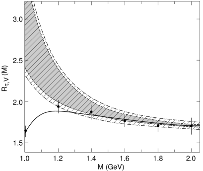
Figure 1: $R_{\tau,V}$ as a function of $M\equiv M_{\tau}$.

Allowing the value of $\alpha_{s}(M_{\tau}^{2})$ to change in the range (29), one gets the larger region between the two dot-dashed curves in Figure 1. For $M\sim M_{\tau}$, the theoretical uncertainty is dominated by the uncertainty in the input value of $\alpha_{s}(M^{2}_{\tau})$; the error on $\delta^{(6)}_{V}$ becomes dominant for $M<1.6$ GeV, and overwhelms the result for $M<$ 1.2 GeV.

One can notice that there is a good agreement between the QCD predictions and the $e^{+}e^{-}$ data points for $M\geq 1.2$ GeV. This confirms the role of the threshold factor $(1-s/M^{2})^{2}$, which minimizes the theoretical uncertainties near the physical cut, and further supports the theoretical framework used to analyze the $\tau$ hadronic width.

The departure of the theoretical prediction from the data points below 1.2 GeV signals the important role of higher-order power corrections in this region. The subleading dimension-8 correction has been neglected before because, at the $\tau$-mass scale, its contribution is expected to be smaller than the uncertainty on $\delta^{(6)}_{V}$. However, when going to smaller values of $M$, the $\delta^{(8)}_{V}(M)$ contribution increases much faster than the dimension-6 one and at some point would even become dominant, indicating a breakdown of the expansion in powers of $1/M$. We can use the lower-mass data points to make an estimate of the size of this contribution. Taking $\alpha_{s}(M_{\tau}^{2})=0.33$ and $\delta^{(6)}_{V}=0.024$, a quite reasonable fit is obtained for $\delta^{(8)}_{V}=-0.0095$. This is shown by the continuous curve in Figure 1. Although the $\delta^{(8)}_{V}(M)$ correction is tiny at $M=M_{\tau}$, its effect changes completely the predicted behaviour below 1.2 GeV. Note, however, that for this value of $\delta^{(8)}_{V}$ one has $\delta^{(8)}_{V}(M)/\delta^{(6)}_{V}(M)=-1.25$ at $M=1$ GeV, which puts some doubts on the applicability of the inverse power expansion at such a low scale. If one takes only into account the region above 1.2 GeV, the size of the experimental error bars does not allow us to make a clear statement about the size of $\delta^{(8)}_{V}$ ($\delta^{(8)}_{V}=0$ is compatible with the data), although smaller values of $\delta^{(8)}_{V}$ seem to be preferred.

3.3 Hadronic invariant-mass distribution

The leading non-perturbative contributions to $R_{\tau}$ are suppressed by a factor of $1/M_{\tau}^{6}$ and, therefore, are very small. Nevertheless they introduce a small uncertainty in the predictions, since their actual evaluation involves a mixture of experimental measurements and theoretical considerations, which are model-dependent to some extent. It would be better to directly measure this contribution from the $\tau$-decay data themselves. This information can be extracted [28] from the invariant-mass distribution of the final hadrons in $\tau$ decay.

Although the distributions themselves cannot be predicted at present, certain weighted integrals of the hadronic spectral functions can be calculated in the same way as $R_{\tau}$. The analyticity properties of $\Pi^{(J)}_{ij,V/A}$ imply [28, 29]:

$$\int_{0}^{s_{0}}ds\,W(s)\,\mbox{\rm Im}\Pi^{(J)}_{ij,V/A}=\qquad\qquad\qquad$$

$$\qquad\qquad\qquad{i\over 2}\oint_{|s|=s_{0}}ds\,W(s)\,\Pi^{(J)}_{ij,V/A},$$ (34)

with $W(s)$ an arbitrary weight function without singularities in the region $|s|\leq s_{0}$. Generally speaking, the accuracy of the theoretical predictions can be much worse than the one of $R_{\tau}$, because non-perturbative effects are not necessarily suppressed. In fact, choosing an appropriate weight function, non-perturbative effects can even be made to dominate the final result. But this is precisely what makes these integrals interesting: they can be used to measure the parameters characterizing the non-perturbative dynamics.

To perform an experimental analysis, it is convenient to use moments of the directly measured invariant-mass distribution [29] ($k,l\geq 0$)

$$R^{kl}_{\tau}(s_{0})\equiv\int_{0}^{s_{0}}\,ds\,\left(1-{s\over s_{0}}\right)^{k}\left({s\over M_{\tau}^{2}}\right)^{l}{dR_{\tau}\over ds}.$$ (35)

The factor $(1-s/s_{0})^{k}$ supplements $(1-s/M_{\tau}^{2})^{2}$ for $s_{0}\not=M_{\tau}^{2}$, in order to squeeze the integrand at the crossing of the positive real-axis and, therefore, improves the reliability of the OPE analysis; moreover, for $s_{0}=M_{\tau}^{2}$ it reduces the contribution from the tail of the distribution, which is badly defined experimentally. A combined fit of different $R_{\tau}^{kl}(s_{0})$ moments results in experimental values for $\alpha_{s}(M_{\tau}^{2})$ and for the coefficients of the inverse-power corrections in the OPE.

The first experimental study has been done by ALEPH [30], using the moments (0,0), (1,0), (1,1), (1,2) and (1,3). $R^{00}=R_{\tau}$ uses the overall normalization of the hadronic distribution, while the ratios $D_{\tau}^{kl}=R^{kl}_{\tau}/R_{\tau}$ are based on the shape of the $s$ distribution and are more dependent on non-perturbative effects [29]. The resulting strong coupling constant measurement [30], $\alpha_{s}(M_{\tau}^{2})=0.330\pm 0.046$, is in excellent agreement with the $R_{\tau}$ determination in Eq. (29). Moreover, the ALEPH analysis has determined the total non-perturbative contribution to $R_{\tau}$ to be [30]

$$\delta_{\mbox{\rm\scriptsize NP}}=(0.3\pm 0.5)\%,$$ (36)

confirming the predicted [4] suppression of non-perturbative corrections.

More recently, ALEPH [31] and CLEO [32] have reported preliminary results of two independent analyses, with a much larger data sample. Although their measured $s$-distributions are in excellent agreement [31], the fitted $\alpha_{s}$ values, shown in Table 5, disagree by about 2 standard deviations. The origin of the discrepancy stems from their different normalizations. While CLEO uses the world-averaged $B_{l}$ values quoted by the Particle Data Group [8], ALEPH has smaller (and precise) leptonic branching ratios and therefore a larger $\tau$ hadronic width, $R_{\tau}=3.645\pm 0.024$. The average of the ALEPH and CLEO $\alpha_{s}(M_{\tau}^{2})$ determinations,

$$\alpha_{s}(M_{\tau}^{2})=0.335\pm 0.016\,,$$ (37)

nicely reproduces the result (29), obtained from $R_{\tau}$ using the theoretical estimates of the small non-perturbative corrections. Nevertheless, the error in (37) should probably be increased by a factor of 2, to account for the present $2\sigma$ discrepancy between the individual measurements.

In addition to confirm that the total non-perturbative correction to $R_{\tau}$ is indeed small, the moment analysis allows to make a determination of the $D=4$ gluon condensate (which does not play any role in $R_{\tau}$), in good agreement with the previous phenomenological estimate $\langle{\alpha_{s}\over\pi}GG\rangle=0.02\pm 0.01$ GeV⁴ [2, 4].

Table 5: Fitted values of $\alpha_{s}(M_{\tau}^{2})$ and the non-perturbative corrections. $\langle{\alpha_{s}\over\pi}GG\rangle$ is given in units of GeV⁴

ALEPH CLEO $\alpha_{s}(M_{\tau}^{2})$ $0.355\pm 0.021$ $0.309\pm 0.024$ $\langle{\alpha_{s}\over\pi}GG\rangle$ $0.006\pm 0.012$ $0.024\pm 0.010$ $\phantom{-}\delta^{(6)}$ $0.006\pm 0.006$ $0.014\pm 0.004$ $-\delta^{(8)}$ $0.0017\pm 0.0014$ $0.0028\pm 0.0006$ $\chi^{2}/\mbox{\rm d.o.f.}$ 0.002 2.1

4 THEORETICAL UNCERTAINTIES

The accuracy of the experimental data is obviously going to improve in the near future. Thus, the final error in the determination of $\alpha_{s}(M_{\tau}^{2})$ will be limited by the accuracy of the theoretical calculation. It is then important to carefully study the possible sources of theoretical uncertainties and try to pin down their numerical effects.

4.1 Higher-order perturbative corrections

The precision of the perturbative calculation of $R_{\tau}$ has been extensively discussed in ref. [5]. Once the important higher-order logarithmic effects have been properly identified and resummed to all orders, the size of the remaining renormalization scheme (and scale) dependence is quite small. The only relevant perturbative uncertainties come from the unknown higher-order coefficients $K_{n>3}$. We have estimated their numerical effect by assuming an algebraic growth of these coefficients and, moreover, in order to be conservative, we have further increased this estimate by a factor of two [6], i.e. $K_{4}\sim 2(K_{3}/K_{2})K_{3}\approx 50$:

$$\Delta(\delta^{(0)})=\pm K_{4}\,A^{(4)}(\alpha_{s})=\pm 0.008\,.$$ (38)

Clearly, this is an arbitrary prescription, but it is probably the most conservative one in the absence of a direct calculation of $K_{4}$. Note, that this value of $K_{4}$ corresponds already to a non-convergent perturbative series:

$$K_{3}\,A^{(3)}(\alpha_{s})=0.010\sim K_{4}\,A^{(4)}(\alpha_{s}).$$ (39)

A recent estimate of $K_{4}$, based on the application of scheme-invariant methods such as the principle of minimal sensitivity [33] or the effective charges approach [34], finds [35] $K_{4}=27.46$. A similar value $K_{4}=29\pm 4\pm 2$ has been obtained from a direct fit to the experimental data [36]. The two estimates are indeed smaller than our conservative choice $K_{4}=50$.

4.2 Renormalons

Possible uncertainties related to the asymptotic (at best) nature of the QCD perturbative expansions at large orders have been considered recently [37, 38, 39, 40, 41, 42, 43, 44, 45, 46, 47]. The leading large-order contributions come from the so-called renormalons, which are associated with known singularities [38] in the Borel transform

$${\cal B}[D]\equiv\tilde{D}(b)={1\over 4\pi^{2}}\sum_{n=0}K_{n+1}{b^{n}\over n!}$$ (40)

of $D(a)=\sum_{n}K_{n}a^{n}/(4\pi^{2})$, where $a\equiv\alpha_{s}/\pi$. In terms of Feynman graphs, the renormalons correspond to inserting a chain of quark-loop bubbles into a gluonic line. Diagrams of this kind generate a factorial growth of the perturbative $D(a)$ series (i.e. $K_{n}\sim n!$) at large orders. Owing to the explicit $1/n!$ factor in the coefficients of (40), $\tilde{D}(b)$ is a much better behaved series. Thus, one could hope to define $D(a)$ through its Borel sum

$$D(a)-D(0)=\int_{0}^{\infty}db\,\tilde{D}(b)\,\exp{(-b/a)}\,.$$ (41)

Unfortunately, the function $\tilde{D}(b)$ has singularities at $b=mb_{0}\equiv 2m/(-\beta_{1})\,$ ($m=-1,\pm 2,\pm 3,...$) and therefore the integral (41) is not defined.

The singularities at $m=+2,+3,...$ (infrared renormalons) are generated by the low-momenta behaviour of these higher-order diagrams, which produces contributions of the form $D(a)\sim\sum_{n}n!\,(a/mb_{0})^{n}$; i.e. $\tilde{D}(b)\sim-mb_{0}/(b-mb_{0})$ for $b<mb_{0}$. The pole at $b=mb_{0}$ gives rise to an ambiguity when one tries to reconstruct $D(a)$ from $\tilde{D}(b)$: [$1/a\approx-\beta_{1}\log{(\sqrt{s}/\Lambda)}$]

$$\delta D(a)\sim\exp{(-mb_{0}/a)}\sim\left(\Lambda^{2}/s\right)^{m}\,.$$ (42)

These infrared $1/s^{m}$ contributions are reabsorbed [38, 39, 40] into the non-perturbative terms of the OPE.

The absence of a singularity at $m=1$ is in fact related to the lack of any physical gauge-invariant local operator of dimension 2. This was challenged in ref. [41], where the relation ${\cal B}[\mbox{\rm Im}\Pi](b)\sim[\sin{\left(\pi b/b_{0}\right)}/\left(\pi b/b_{0}\right)]\,\tilde{D}(b)$ was established, implying that either $\tilde{D}(b)$ has a pole corresponding to $m=1$ or ${\cal B}[\mbox{\rm Im}\Pi](b)$ has a zero at that point. The first possibility (an infrared renormalon for $m=1$) would imply a $1/s$ ambiguity which could not be reabsorbed by the OPE. This puzzle has been clarified by the exact calculation of $\tilde{D}(b)$ (both in QED [42] and in QCD [43]) in the limit of a large number of quark flavours, which shows that there is no infrared renormalon corresponding to $m=1$, and ${\cal B}[\mbox{\rm Im}\Pi](b)$ has in fact a zero. This confirms the relation of infrared renormalons to gauge-invariant operators [38, 39, 40].

The ultraviolet renormalons ($m=-1,...$) are generated by the high-momenta behaviour and, because of asymptotic freedom, give rise to a Borel-summable series (they are in the negative real axis, outside the integration region), which makes them harmless. They don’t put any real limit [38] to the applicability of perturbation theory. Nevertheless, if the Borel summation is not performed, the ultraviolet renormalons induce an intrinsic uncertainty in the truncated perturbative series.

The factorial growth of the perturbative series is indeed dominated by the contribution of the leading ultraviolet renormalon ($m=-1$), $K_{n}\sim n!/(-b_{0})^{n}$, which gives rise to an asymptotic series:

$$|K_{1}a|>|K_{2}a^{2}| \!\!\!\!> \!\!\!\!\ldots>|K_{N-1}a^{N-1}|\sim|K_{N}a^{N}|$$

$$<|K_{N+1}a^{N+1}| \!\!\!\!< \!\!\!\!\ldots$$ (43)

The successive terms decrease until $N\sim b_{0}/a$, where the minimum value is attained, and the series explodes afterwards. The alternating sign of the $K_{n}$ coefficients guarantees that the series is Borel-summable. However, if one only considers the truncated series at a given finite order, the accuracy is obviously limited by the size of the minimum term [44]:

$$4\pi^{2}\,\delta D(a) \!\!\!\!\equiv \!\!\!\!|K_{N}a^{N}|\sim N!\,N^{-N}\sim\sqrt{2\pi N}\,\rm e^{-N}$$ (44)

$$\!\!\!\!\sim \!\!\!\!\exp{(-b_{0}/a)}\sim\Lambda^{2}/s\,.$$

Thus, the $m=-1$ ultraviolet renormalon seems to induce an uncertainty in the perturbative series, which scales like $1/s$. This has been used [45, 46] to advocate for an additional (small) uncertainty in $R_{\tau}$ proportional to $1/M_{\tau}^{2}$; such a conclusion is incorrect, because:

1. As it stands, the estimate (44) depends on the chosen renormalization scheme (the definition of $\Lambda$). A more careful analysis [47] shows that the ambiguity actually scales as $A\sqrt{\alpha_{s}(\mu^{2})}\Lambda^{2}s/\mu^{4}$, where the scheme dependence has been absorbed into the factor $A$. The result (44) only follows if one takes $\mu^{2}=s$. Keeping an arbitrary renormalization scale $\mu$, the $\Lambda^{2}s/\mu^{4}$ term does not contribute to the close-contour integral (9) defining $R_{\tau}$ (Cauchy theorem).

2. One could still argue [46] that the improved perturbative series, which resums higher-order logarithms through the $A^{(n)}(\alpha_{s})$ functions in Eq. (16), takes $\mu^{2}=s$ and thus the $1/M_{\tau}^{2}$ ambiguity comes back. However, it was shown in ref. [5] that the scale dependence of the resummed perturbative result is tiny; taking $\mu=\xi\sqrt{s}$, the difference between $\xi=1$ and $\xi=3$ is very small. A $\Lambda^{2}/(\xi^{2}M_{\tau}^{2})$ term would instead change by a factor of 9, making such a contribution irrelevant for $\xi\sim 3$.

3. Eq. (44) is just an estimate of the ultimate perturbative error, defined as the size of the minimum term. At the $M_{\tau}$ scale, $a\approx 0.1$ and therefore $N\sim 2/(-\beta_{1}a)\sim 4$, which by no means is a large number; thus, one could question the large-$N$ approximations used to obtain the result. However, the important point is that one is in fact assuming that $|K_{3}a^{3}|>|K_{4}a^{4}|>|K_{N}a^{N}|$, i.e. the so-called ultraviolet-renormalon effect is by definition smaller than the usual perturbative error. It only gives a crude estimate of the maximum accuracy which can be obtained by computing higher-orders in perturbation theory. It is not a new source of uncertainty, but just a lower bound on the same perturbative error.

Any possible ultraviolet renormalon ambiguity is therefore already included in the perturbative error quoted in Eq. (38). Taking an extremely conservative attitude, one could argue that the onset of the asymptotic behaviour of the perturbative series has been perhaps reached already at $N=3$. Although, there is no signal of such behaviour in the presently known terms, the possibility of a large $N=4$ contribution cannot be excluded. If that were the case, one should then take the size of the known $N=3$ term (and not a rough large-$N$ approximation to it!) as the ultimate uncertainty of the truncated perturbative calculation. As explicitly shown in Eq. (39), the conservative perturbative error (38) we have been adopting [6] in the actual $R_{\tau}$ calculation, already includes such a pathological possibility.

4.3 Charm corrections

Since the $\tau$ mass is below the charm-production threshold, the calculation of $R_{\tau}$ has been performed in the effective QCD theory with only 3 active quark flavours. The decoupling of heavy quarks from the non-singlet currents [49] guarantees that the leading (logarithmic) charm-quark effects can be reabsorbed into the QCD running coupling [50]. These contributions are then taken into account, through the matching relation between the values of $\alpha_{s}$ in the effective theories with 3 and 4 flavours [51, 52]. Nevertheless, there are additional corrections suppressed by inverse powers of the heavy-quark mass, which a priori could be sizeable. These effects appear first at ${\cal O}(\alpha_{s}^{2})$, through a virtual $c$-$\bar{c}$ vacuum-polarization contribution to the gluon propagator. The charm-quark contribution is fully known at ${\cal O}(\alpha_{s}^{2})$ [53, 54] and the ${\cal O}\left[\alpha_{s}^{3}\left(M_{\tau}/m_{c}\right)^{n}\right]$ contributions with $n=1,2$ and $3$ have been recently computed [52]. The final numerical effect is very small [52, 53, 54]:

$$\Delta_{c} \!\!\!\!\!= \!\!\!\!\!\left({\alpha_{s}\over\pi}\right)^{2}{M_{\tau}^{2}\over m_{c}^{2}}\left[{1\over 225}\log{\left({m_{c}^{2}\over M_{\tau}^{2}}\right)}+{107\over 4500}+\ldots\right]$$ (45)

$$\!\!\!\!\approx \!\!\!\!0.0004\,.$$

4.4 Non-perturbative corrections

The experimental data has already shown that the total non-perturbative correction to $R_{\tau}$ is small [see Eq. (36)], in agreement with the theoretical prediction. Nevertheless, with the present experimental accuracy, inverse power corrections introduce an uncertainty of about 1%.

On the theoretical side, it is clear that those corrections are very suppressed (either by a factor $1/M_{\tau}^{6}$ or $\alpha_{s}^{2}/M_{\tau}^{4}$); however, the actual estimate of the leading contribution in Eq. (21) relies on phenomenological fits. The main source of information has been up to now $e^{+}e^{-}$ data, which only measures $\delta^{(6)}_{ij,V}$. In order to estimate the axial contribution, one needs to assume $\delta^{(6)}_{ij,A}/\delta^{(6)}_{ij,V}\approx-11/7$, as predicted by factorization. While the opposite sign of the vector and axial-vector $D=6$ contributions (helicity flip) does not depend on that approximation, the magnitude of their ratio is changed by non-factorizable corrections. Those non-factorizable radiative contributions have been found to be small [55] (in the $\overline{MS}$ scheme with a naïve anticommuting $\gamma_{5}$). Nevertheless, it would be desirable to have a direct experimental measurement.

The preliminary fits of the $\tau$-decay hadronic distribution, given in Table 5, result in a value of $\delta^{(6)}$ which has the predicted magnitude but the wrong sign. However, given the present size of the experimental error bars and the strong correlation between the different fit parameters, one can only conclude that $\delta^{(6)}$ is in fact small.

From the difference between the measured semi-inclusive $\tau$ hadronic widths in Eq. (3.1), $R_{\tau,V}-R_{\tau,A}=0.10\pm 0.07$, it is possible to extract the value of $\delta^{(6)}_{V-A}$. Note that the perturbative contributions cancel in this difference. Taking into account the small $D=2$ and $D=4$ corrections [4], one gets $\delta^{(6)}_{V-A}=(6\pm 5)\%$, in good agreement with the theoretical estimate in Eq. (21). However, the present errors are too large for this determination to be significant. Clearly, better data is required.

There is another source of non-perturbative contributions, which has been recently analyzed: instantons [56, 57]. It is well-known that instantons do spoil the OPE by introducing corrections that are power-suppressed by 9 or more inverse powers of the momentum. Owing to this large power suppression, the instanton contributions are very sensitive to the momentum scale: they are either negligible, and therefore irrelevant for practical applications, or very large, in which case they destroy the convergence of the OPE. Thus, instantons just provide a lower limit to the momentum scale at which the OPE can be applied.

The existing analyses [56, 57] indicate that the instanton contribution to $R_{\tau}$ is tiny. Unfortunately, it is difficult to make reliable quantitative predictions. For $\alpha_{s}(M_{\tau}^{2})=0.32$, the instanton effect could reach the 0.2–0.3% level [57], but the theoretical estimates are no longer valid at larger $\alpha_{s}$ values. Nevertheless, the instanton contributions to $R_{\tau,V}$ and $R_{\tau,A}$ are predicted to be much larger than the total correction to $R_{\tau}$ [57] (there is a cancellation between the vector and axial-vector contributions to $R_{\tau}$, similar to the one occurring in $\delta^{(6)}$). The possible size of the instanton effect can then be bounded using the present information on $R_{\tau,V/A}$.

The data points in Figure 1 have a very soft dependence on the energy scale, which discards any sizable instanton contribution above 1.2 GeV. Moreover, a recent phenomenological analysis of $R_{\tau,V}-R_{\tau,A}$, where the instanton effect is supposed to be maximal, concludes [58] that the instanton contribution to $R_{\tau}$ is smaller then 0.0005.

4.5 Uncertainties in the running of $\alpha_{s}$

The final determination of $\alpha_{s}(M_{\tau}^{2})$ has to be compared with the values of $\alpha_{s}$ measured at other scales, for instance $\alpha_{s}(M_{Z}^{2})$. The correct way of running the strong coupling through the different physical thresholds ($c$, $b$, …) at ${\cal O}(\alpha_{s}^{3})$ was known already twelve years ago [51]. One considers two different strong couplings, $\alpha_{s}^{(f)}$ and $\alpha_{s}^{(f-1)}$, in the effective QCD theories with $N_{f}$ and $N_{f-1}$ active flavours, and imposes a series of matching conditions [51, 52] which guarantee that the same physical predictions are obtained in both theories. Contrary to common belief, the $\overline{MS}$ strong coupling is (in general) not continuous at the matching point [51]. The exact point where the matching between both theories is performed is actually irrelevant [59], provided one does not choose a crazy $\mu/m_{q}(\mu^{2})$ ratio which would induce huge higher-order corrections.

Taking $\alpha_{s}(M_{\tau}^{2})=0.33$ as input, the resulting value of $\alpha_{s}(M_{Z}^{2})$ changes by less than 0.5% if the $b$-threshold matching point is varied between 2 and 40 GeV, or if one changes the $c$-threshold between $M_{\tau}$ and $m_{b}$. Note that the usual incorrect procedure [45] of requiring a continuous $\alpha_{s}$ largely overestimates this error.

The matching conditions take correctly into account the logarithmic heavy-quark corrections. The physical observables get in addition $1/m_{q}^{n}$ contributions that need to be computed. It has been advocated [45, 46] that the uncertainty associated with these quark-mass effects can be estimated through a generous variation of the matching point. This is not quite correct. Varying the matching point, one is only testing the $\mu$-dependence of the logarithmic corrections. Assuming that one knows the matching conditions to a sufficiently high order, the variation of $\mu$ would not produce any numerical change (i.e. zero error!); but heavy-quark effects would be of course still there.

In fact, within the $\overline{MS}$ scheme, the $1/m_{q}^{n}$ contributions have nothing to do with the running of $\alpha_{s}$. The renormalization group equations only involve logarithms, because $\overline{MS}$ is a mass-independent renormalization scheme. Mass effects are of course taken into account in the explicit calculation of each physical observable, as discussed in Sect. 4.3. The induced correction to $R_{\tau}$, given in Eq. (45), is very small.

5 SUMMARY

Because of its inclusive nature, the total hadronic width of the $\tau$ can be rigorously computed within QCD. One only needs to study two-point correlation functions for the vector and axial-vector currents. As shown in Eq. (9), this information is only needed in the complex plane, away from the time-like axis; the dangerous region near the physical cut does not contribute at all to the result, because of the phase-space factor $(1-s/M_{\tau}^{2})^{2}$. The uncertainties of the theoretical predictions are then quite small. Notice that the accuracy of the $R_{\tau}$ predictions is much better than the corresponding estimate of $R_{e^{+}e^{-}}(s)$ at $s=M_{\tau}^{2}$ [$R_{e^{+}e^{-}}(s)$ measures the vector spectral function on the physical cut, where the theoretical predictions (at least at low energies) are more uncertain].

The ratio $R_{\tau}$ is very sensitive to the value of the strong coupling, and therefore can be used to measure $\alpha_{s}(M_{\tau}^{2})$ [2]. This observation has triggered an ongoing effort to improve the knowledge of $R_{\tau}$ from both the experimental and the theoretical sides. The fact that $M_{\tau}$ is a quite low energy-scale (i.e. that $\alpha_{s}(M_{\tau}^{2})$ is big), but still large enough to allow a perturbative analysis, makes $R_{\tau}$ an ideal observable to determine the QCD coupling. Moreover, since the error of $\alpha_{s}(\mu^{2})$ shrinks as $\mu$ increases, the good accuracy of the $R_{\tau}$ determination of $\alpha_{s}(M_{\tau}^{2})$ implies a very precise value of $\alpha_{s}(M_{Z}^{2})$.

The theoretical analysis of $R_{\tau}$ has reached a very mature level. Many different sources of possible perturbative and non-perturbative contributions have been analyzed in detail. As shown in the previous section, the final theoretical uncertainty is small and has been adequately taken into account in the final $\alpha_{s}(M_{\tau}^{2})$ determination in Eq. (29). (Note, however, that there are still sizeable fluctuations in the $B_{l}$ measurements [31], which could slightly modify the final result).

The comparison of the theoretical predictions with the experimental data shows a successful and consistent picture. The $\alpha_{s}(M_{\tau}^{2})$ determination is in excellent agreement with the measurements at the $Z$-mass scale, providing clear evidence of the running of $\alpha_{s}$. Moreover, the analysis of the semi-inclusive components of the $\tau$ hadronic width, $R_{\tau,V}$, $R_{\tau,A}$ and $R_{\tau,S}$, and the invariant-mass distribution of the final decay products gives a nice confirmation of the reliability of the theoretical framework.

References

- [1] E. Braaten, Phys. Rev. Lett. 60 (1988) 1606; Phys. Rev. D39 (1989) 1458.
- [2] S. Narison and A. Pich, Phys. Lett. B211 (1988) 183.
- [3] A. Pich, Hadronic Tau-Decays and QCD, in Proc. Workshop on Tau Lepton Physics (Orsay, 1990), eds. M. Davier and B. Jean-Marie (Ed. Frontières, Gif-sur-Yvette, 1991), p. 321.
- [4] E. Braaten, S. Narison and A. Pich, Nucl. Phys. B373 (1992) 581.
- [5] F. Le Diberder and A. Pich, Phys. Lett. B286 (1992) 147.
- [6] A. Pich, QCD Predictions for the Tau Hadronic Width and Determination of , in Proc. Second Workshop on Tau Lepton Physics (Ohio, 1992), ed. K.K. Gan (World Scientific, Singapore, 1993), p. 121.
- [7] S. Narison, from Tau Decays, in Proc. Third Workshop on Tau Lepton Physics (Montreux, 1994).
- [8] Particle Data Group, Review of Particle Properties, Phys. Rev. D50 (1994) 1173.
- [9] M.A. Shifman, A.L. Vainshtein and V.I. Zakharov, Nucl. Phys. B147 (1979) 385.
-
[10]
T.L. Trueman, Phys. Lett. 88B (1979) 331;
A.I. Antoniadis, Phys. Lett. 84B (1979) 223. -
[11]
K.G. Chetyrkin, A.L. Kataev and F.V. Tkachov, Phys. Lett. 85B (1979) 277;
M. Dine and J. Sapirstein, Phys. Rev. Lett. 43 (1979) 668;
W. Celmaster and R. Gonsalves, Phys. Rev. Lett. 44 (1980) 560. - [12] S.G. Gorishny, A.L. Kataev and S.A. Larin, Phys. Lett. B259 (1991) 144.
- [13] L.R. Surguladze and M.A. Samuel, Phys. Rev. Lett. 66 (1991) 560.
- [14] J. Chýla, A. Kataev and S. Larin, Phys. Lett. B267 (1991) 269.
- [15] A.A. Pivovarov, Z. Phys. C53 (1992) 461.
- [16] K.G. Chetyrkin and A. Kwiatkowski, Z. Phys. C59 (1993) 525.
- [17] W.J. Marciano and A. Sirlin, Phys. Rev. Lett. 61 (1988) 1815; 56 (1986) 22.
- [18] E. Braaten and C.S. Li, Phys. Rev. D42 (1990) 3888.
- [19] A. Pich, Nucl. Phys. B (Proc. Suppl.) 31 (1993) 213.
-
[20]
B.R. Webber, QCD and Jet Physics,
in Proc. XXVII Int. Conf. on High Energy Physics (Glasgow, 1994);
S. Bethke, Summary of Measurements, these proceedings. -
[21]
R. Akers et al. (OPAL), Phys. Lett. B328 (1994) 207;
M. Artuso et al. (CLEO), Phys. Rev. Lett. 72 (1994) 3762;
M. Procario et al. (CLEO), Phys. Rev. Lett. 70 (1993) 1207;
D. Decamp et al. (ALEPH), Z. Phys. C54 (1992) 211. - [22] Gibaut et al. (CLEO), Phys. Rev. Lett. 73 (1994) 934.
-
[23]
D. Buskulic et al. (ALEPH), Phys. Lett. B332 (1994) 209; 219;
R. Akers et al. (OPAL), CERN-PPE/94-108 (Phys. Lett. B);
M. Battle et al. (CLEO), Phys. Rev. Lett. 73 (1994) 1079;
D. Bauer et al. (TPC/), Phys. Rev. D50 (1994) R13. -
[24]
D. Groom and K. Hayes, in Proc.
Third Workshop on Tau Lepton Physics (Montreux, 1994);
R. Alemany, Tau Decays into Kaons, in Proc. XXVII Int. Conf. on High Energy Physics (Glasgow, 1994). -
[25]
Y.S. Tsai, Phys. Rev. D4 (1971) 2821.
H.B. Thacker and J.J. Sakurai, Phys. Lett. 36B (1971) 103. - [26] S. Narison and A. Pich, Phys. Lett. B304 (1993) 359.
- [27] S.I. Eidelman and V.N. Ivanchenko, Phys. Lett. B257 (1991) 437; Proc. Third Workshop on Tau Lepton Physics (Montreux, 1994).
- [28] A. Pich, QCD Tests From Tau Decay Data, in Proc. Tau-Charm Factory Workshop (SLAC, 1989), ed. L.V. Beers, SLAC-Report-343 (1989), p. 416.
- [29] F. Le Diberder and A. Pich, Phys. Lett. B289 (1992) 165.
- [30] D. Buskulic et al. (ALEPH), Phys. Lett. B307 (1993) 209.
- [31] L. Duflot, QCD Tests From Tau Decays, these proceedings.
- [32] R. Stroynowski, Measurement of Hadronic Spectral Moments in Decays and Determination of , in Proc. XXVII Int. Conf. on High Energy Physics (Glasgow, 1994).
- [33] P.M. Stevenson, Phys. Rev. D23 (1981) 2916.
- [34] G. Grunberg, Phys. Lett. B221 (1980) 70; Phys. Rev. D29 (1984) 2315.
- [35] A.L. Kataev and V.V. Starshenko, CERN-TH.7198/94; and these proceedings.
- [36] F. Le Diberder, Experimental Estimates of Higher-Order Perturbative Corrections, these proceedings.
- [37] G.B. West, Phys. Rev. Lett. 67 (1991) 1388; 67 (1991) 3732(E).
- [38] A.H. Mueller, Phys. Lett. B308 (1993) 355; Nucl. Phys. B250 (1985) 327; The QCD Perturbation Series, in Proc. QCD – 20 Years Later (Aachen, 1992), ed. P.M. Zerwas and H.A. Kastrup (World Scientific, Singapore, 1993), Vol. 1, p. 162.
- [39] G. Grunberg, Phys. Lett. B325 (1994) 441; these proceedings.
- [40] F. David, Nucl. Phys. B234 (1984) 237.
-
[41]
L.S. Brown and L.G. Yaffe, Phys. Rev. D45 (1992)
R398;
L.S. Brown, L.G. Yaffe and Ch. Zhai, Phys. Rev. D46 (1992) 4712. - [42] M. Beneke, Nucl. Phys. B405 (1993) 424.
- [43] C.N. Lovett-Turner and C.J. Maxwell, DTP/94/58.
- [44] V.I. Zakharov, Nucl. Phys. B385 (1992) 452.
- [45] G. Altarelli, in Proc. QCD – 20 Years Later (Aachen, 1992), ed. P.M. Zerwas and H.A. Kastrup (World Scientific, Singapore, 1993), Vol. 1, p. 172.
- [46] G. Altarelli, in Proc. Third Workshop on Tau Lepton Physics (Montreux, 1994).
- [47] M. Beneke and V.I. Zakharov, Phys. Rev. Lett. 69 (1992) 2472.
- [48] A.I Vainshtein and V.I. Zakharov, Phys. Rev. Lett. 73 (1994) 1207.
- [49] T. Appelquist and J. Carazzone, Phys. Rev. D11 (1975) 2856.
-
[50]
S. Weinberg, Phys. Lett. B91 (1980) 51;
B. Ovrut and H. Schnitzer, Nucl. Phys. B189 (1981) 509. - [51] W. Bernreuther and W. Wetzel, Nucl. Phys. B197 (1982) 228.
- [52] S.A. Larin, T. van Ritbergen and J.A.M. Vermaseren, NIKHEF-H/94-30.
- [53] K.G. Chetyrkin, Phys. Lett. B307 (1993) 169.
- [54] D.E. Soper and L.R. Surguladze, University of Oregon preprint OITS 545.
- [55] L.-E. Adam and K.G. Chetyrkin, Phys. Lett. B329 (1994) 129.
-
[56]
P. Nason and M. Porrati, Nucl. Phys. B421 (1994) 518;
P. Nason and M. Palassini, CERN preprint CERN-TH.7483/94. - [57] I.I. Balitsky, M. Beneke and V.M. Braun, Phys. Lett. B318 (1993) 371.
- [58] V. Kartvelishvili and M. Margvelashvili, Ferrara preprint INFN-FE 08-94.
-
[59]
W. Bernreuther, Threshold Effects on the QCD Coupling,
Aachen preprint PITHA 94/31;
G. Rodrigo and A. Santamaria, Phys. Lett. B313 (1993) 441.