INLO–PUB–14/94 P.J. Rijken and W.L. van Neerven August 1994

Order $\alpha_{s}^{2}$ contributions to the Drell-Yan cross section at fixed target energies

1 Introduction

Massive lepton pair production in hadronic interactions is besides deep inelastic lepton-hadron scattering one of the most important probes of the structure of hadrons. It is well established that one of the dominant production mechanisms is the Drell-Yan (DY) process [1]. Here the lepton pair is the decay product of one of the electroweak vector bosons of the standard model ($\gamma^{\ast},W$ and $Z$) which in the Born approximation are produced by the annihilation of quarks and anti-quarks coming from the colliding hadrons. This process is of experimental interest because it provides us with an alternative way to measure the parton densities of the proton and neutron which have been very accurately determined by the deep inelastic lepton hadron experiments. Moreover it enables us to measure the parton densities of unstable hadrons like pions and kaons which is impossible in deep inelastic lepton-hadron scattering. Besides the measurement of the parton densities there are other important tests of perturbative quantum chromo dynamics (QCD) which can be carried out by studying the DY process. Here we want to mention the scale evolution of the parton densities, although not observed in this process because of the low statistics, and the measurement of the running coupling constant $\alpha_{s}(\mu^{2})$ which includes the QCD scale $\Lambda$. Finally this process constitutes an important background for other production mechanisms of lepton pairs. Examples are $J/\Psi$ and $\Upsilon$ decays or thermal emission of lepton pairs in heavy-ion collisions [2].
The DY process is also of theoretical interest. Since it is one of the few reactions which can be calculated up to second order in perturbation theory it enables us to study the origin of large QCD corrections which are mostly due to soft gluon bremsstrahlung and virtual gluon contributions. In order to control these corrections in the perturbation series one has constructed various kinds of resummation techniques mostly leading to the exponentiation of the dominant terms [3]-[7]. Another issue is the dependence of the physical quantities on the chosen scheme and the choice of scales. Since the perturbation series is truncated the theoretical cross section will depend on the scheme and the renormalization/factorization scale $\mu$. These dependences can be reduced by including higher order terms in the perturbation series. An alternative way is to determine $\mu$ itself (optimum scale) by using so called improved perturbation theory like the principle of minimal sensitivity (PMS) [8], fastest apparent convergence (FAC) [9] or the Brodsky-Lepage-Mackenzie (BLM) procedure [10].
The first fixed target experiment on massive lepton pair production was carried out by the Columbia-BNL group [11]. Later on this process was studied in many other experiments which were carried out at increasing energies (for reviews see [12]). When the statistics of the data was improving one discovered that the cross section could not be described by the simple parton model given by S.D. Drell and T.M. Yan in [1]. This was revealed for the first time by the NA3 experiment [13] (see also [14]) where the data show a discrepancy in the normalization between the experimental and theoretical cross section. This discrepancy is expressed by a so called $K$-factor which is defined by the ratio between the experimentally observed cross section and its theoretical prediction. The above group and the experiments carried out later on [15] show that this $K$-factor ranges between 1.5 and 2.5 and is roughly independent of the type of incoming hadrons. The most generally accepted explanation of this $K$-factor was provided by perturbative QCD. The calculation of the order $\alpha_{s}$ corrections [16]-[19] to the DY cross section in [1] show that a considerable part of the $K$-factor can be attributed to next-to-leading order effects. However the order $\alpha_{s}$ corrections do not account for the whole $K$-factor. More recent experiments [20]-[23] still indicate that the ratio between the experimental cross section and the order $\alpha_{s}$ corrected theoretical prediction is about 1.4, a number which might be explained by including QCD corrections beyond order $\alpha_{s}$ as we will show in this paper.
As has been mentioned at the beginning the DY process is one of the few processes where the order $\alpha_{s}^{2}$ corrections to the coefficient function are completely known. The latter refers to the cross section $d\sigma/dm$ only where $m$ denotes the lepton pair invariant mass. This coefficient function has been calculated in the $\overline{\mbox{MS}}$ [24] as well as in the DIS [25] scheme. However in the case of the double differential cross section $d^{2}\sigma/dmdx_{F}$ ($d^{2}\sigma/dmdy$) one has only calculated the order $\alpha_{s}^{2}$ part of the coefficient function which is due to soft and virtual gluon contributions [26] because the remaining part is very complicate to compute. Fortunately as is shown in the literature [16]-[19] the soft plus virtual gluon corrections dominate the total and differential DY cross sections in particular at fixed target energies so that we can restrict to them to make reliable predictions.
An analysis of the higher order corrections to the total DY cross section for $W$- and $Z$-production at large hadron collider energies has been performed in [24, 25]. Such an analysis is still missing for the DY process at fixed target energies and therefore we present it here. In particular we want to show that the discrepancy in the normalization between the order $\alpha_{s}$ corrected DY cross section and the one measured at the fixed target experiments can be partially explained by including the order $\alpha_{s}^{2}$ contributions due to soft plus virtual gluon effects.
This paper is organized as follows. In section 2 we present the expressions for the various DY cross sections and give a review of the partonic subprocesses included in our analysis. In section 3 the validity of the soft plus virtual gluon approximation will be discussed and we make a comparison between the order $\alpha_{s}^{2}$ corrected cross section and the most recent fixed target DY data. In appendices A and B we give the coefficient functions for $d^{2}\sigma/dmdx_{F}$ ($d^{2}\sigma/dmdy$) corrected up to order $\alpha_{s}$ and order $\alpha_{s}^{2}$ respectively. They are presented for arbitrary renormalization and mass factorization scale in the $\overline{\mbox{MS}}$- as well as in the DIS-scheme.

2 Higher order QCD corrections to $d^{2}\sigma/dmdx_{F}$
($d^{2}\sigma/dmdy$) and $d\sigma/dm$

Massive lepton pair production in hadron-hadron collisions proceeds through the following reaction

$$H_{1}+H_{2}\;\rightarrow V +\hskip 8.53581pt"X"$$ (2.1)

$$\hskip 5.0pt\lfloor\raisebox{-5.9pt}{$\rightarrow$} \ell_{1}+\ell_{2}$$

Here $H_{1}$ and $H_{2}$ denote the incoming hadrons and $V$ is one of the vector bosons of the standard model ($\gamma^{\ast}$,$Z$ or $W$) which subsequently decays into a lepton pair ($\ell_{1}$,$\ell_{2}$). The symbol $"X"$ denotes any inclusive hadronic final state which is allowed by conservation of quantum numbers. Following the QCD improved parton model as originally developed in [1] the double differential DY cross section can be written as

$$\frac{d^{2}\sigma}{dQ^{2}dx_{F}}=\sum_{i,j}\sigma_{V}(Q^{2},M_{V}^{2})\,\int_{x_{1}}^{1}dt_{1}\,\int_{x_{2}}^{1}dt_{2}\,H_{ij}(t_{1},t_{2},\mu^{2})\Delta_{ij}(t_{1},t_{2},x_{1},x_{2},Q^{2},\mu^{2}).$$

(2.2)

Here $Q^{2}=m^{2}$ where $m$ denotes the lepton pair invariant mass. The longitudinal momentum fraction $x_{F}$ of the lepton pair and the Bjørken scaling variable are defined by

$$x_{F}=x_{1}-x_{2}=\frac{2p_{L}}{\sqrt{S}},\hskip 56.9055pt\tau=\frac{Q^{2}}{S}=x_{1}x_{2},$$ (2.3)

where $\sqrt{S}$ stands for the center of mass energy of the incoming hadrons $H_{1}$ and $H_{2}$. The quantity $\sigma_{V}$ is the pointlike DY cross section which describes the process

$$q_{1}+\bar{q}_{2}\rightarrow V\rightarrow\ell_{1}+\ell_{2},$$ (2.4)

where $q_{1}$ and $\bar{q}_{2}$ denote the incoming quark and anti-quark respectively. If we limit ourselves to $V=\gamma^{\ast}$,$Z$ then $\sigma_{V}$ gets the form

$$\sigma_{V}(Q^{2},M_{Z}^{2}) = \frac{4\pi\alpha^{2}}{9Q^{4}}\left[e_{\ell}^{2}e_{q}^{2}+\frac{2Q^{2}(Q^{2}-M_{Z}^{2})}{|Z(Q^{2})|^{2}}e_{\ell}e_{q}C_{V,\ell}C_{V,q}\right.$$ (2.5)

$$\left.+\frac{(Q^{2})^{2}}{|Z(Q^{2})|^{2}}(C_{V,\ell}^{2}+C_{A,\ell}^{2})(C_{V,q}^{2}+C_{A,q}^{2})\right]$$

with

$$Z(Q^{2})=Q^{2}-M_{Z}^{2}+iM_{Z}\Gamma_{Z}.$$ (2.6)

Here the width of the $Z$-boson is taken to be energy independent and all fermion masses are neglected since they are much smaller than $\sqrt{Q^{2}}$. The charges of the leptons and quarks are given by

$$e_{\ell}=-1,\hskip 56.9055pte_{u}=\frac{2}{3},\hskip 56.9055pte_{d}=-\frac{1}{3}.$$ (2.7)

The vector- and axial-vector coupling constants of the $Z$-boson to the leptons and quarks are equal to

$$\begin{array}[]{ll}\displaystyle C_{A,\ell}=\frac{1}{2\sin 2\theta_{W}}&C_{V,\ell}=-C_{A,\ell}(1-4\sin^{2}\theta_{W})\\[8.61108pt] C_{A,u}=-C_{A,d}=-C_{A,\ell}&\\[8.61108pt] C_{V,u}=C_{A,\ell}\left(1-\frac{8}{3}\sin^{2}\theta_{W}\right)&C_{V,d}=-C_{A,\ell}\left(1-\frac{4}{3}\sin^{2}\theta_{W}\right).\end{array}$$ (2.8)

The function $H_{ij}$ in (2.2) stands for the combination of parton densities corresponding to the incoming partons $i$ and $j$ ($i,j=q,\bar{q},g$). Finally $\Delta_{ij}$ denotes the DY coefficient function which is determined by the partonic subprocess

$$i+j\rightarrow V+"X"$$ (2.9)

where $"X"$ now represents any multi partonic final state. Both functions $H_{ij}$ and $\Delta_{ij}$ depend in addition to the scaling variables $t_{i}$ and $x_{i}$ also on the renormalization and mass factorization scales which are usually put to be equal to $\mu$. Besides the cross section in (2.2) one is sometimes also interested in the rapidity distribution of the lepton pair. In this case the left hand side in (2.2) is replaced by $d^{2}\sigma/dQ^{2}dy$ where $y$ denotes the rapidity defined by (see (2.3))

$$y=\frac{1}{2}\ln\frac{x_{1}}{x_{2}},\hskip 28.45274ptx_{1}=\sqrt{\tau}\,e^{\displaystyle y},\hskip 28.45274ptx_{2}=\sqrt{\tau}\,e^{\displaystyle-y}$$ (2.10)

or

$$y=\frac{1}{2}\ln\frac{x_{F}+\sqrt{x_{F}^{2}+4\tau}}{-x_{F}+\sqrt{x_{F}^{2}+4\tau}}.$$ (2.11)

Furthermore on the right hand side the coefficient function $\Delta_{ij}$ is replaced by its analogue corresponding to the cross section $d^{2}\sigma/dQ^{2}dy$.
The coefficient function $\Delta_{ij}$ (2.2) can be expanded as a power series in the running coupling constant $\alpha_{s}(\mu^{2})$ as follows

$$\Delta_{ij}=\sum_{n=0}^{\infty}\left(\frac{\alpha_{s}(\mu^{2})}{4\pi}\right)^{n}\,\Delta_{ij}^{(n)}.$$ (2.12)

In lowest order the coefficient function of the differential cross section (2.2) is determined by the subprocess

$$q+\bar{q}\rightarrow V.$$ (2.13)

Here $V$ either stands for the virtual photon $\gamma^{\ast}$ or the $Z$-boson and the coefficient function is given by

$$\Delta_{q\bar{q}}^{(0)}=\frac{1}{x_{1}+x_{2}}\delta(t_{1}-x_{1})\,\delta(t_{2}-x_{2}).$$ (2.14)

The order $\alpha_{s}$ corrections to the Born process (2.13) denoted by $\Delta_{q\bar{q}}^{(1)}$ are given by the one-loop contributions to (2.13) and the gluon bremsstrahlung process

$$q+\bar{q}\rightarrow V+g.$$ (2.15)

In addition to the process above we have another reaction which instead of a quark or anti-quark has a gluon in the initial state

$$g+q(\bar{q})\rightarrow V+q(\bar{q}).$$ (2.16)

This reaction contributes to $\Delta_{gq}^{(1)}$. Both contributions $\Delta_{q\bar{q}}^{(1)}$ and $\Delta_{gq}^{(1)}$ have been calculated in [17, 18, 27] (DIS-scheme) and in [28] ($\overline{\mbox{MS}}$-scheme) and are presented in (A.1) and (A.7), (A.8) respectively. A part of the order $\alpha_{s}^{2}$ corrections to the coefficient function corresponding to $d^{2}\sigma/dQ^{2}dx_{F}$ has also been calculated in [26]. These corrections originate from the soft plus virtual gluon contributions. They consist of the two-loop corrections to process (2.13) and the one-loop correction to process (2.15) where the gluon is taken to be soft. Furthermore one has also included the bremsstrahlungs process

$$q+\bar{q}\rightarrow V+g+g$$ (2.17)

and fermion pair production

$$q+\bar{q}\rightarrow V+q+\bar{q}$$ (2.18)

where the gluons were taken to be soft and the quark–anti-quark pair in the final state of (2.18) has a low invariant mass.
All above corrections contribute to $\Delta_{q\bar{q}}^{(2)}$ and can be found in appendix B for arbitrary factorization and renormalization scale $\mu$ where they are presented in the $\overline{\mbox{MS}}$- as well as in the DIS-scheme. The hard gluon corrections (2.17) and the other two-to-three body processes (see below) are very hard to compute at least for the double differential cross sections. Fortunately as has been shown in [16]-[19] the bulk of the order $\alpha_{s}$ radiative corrections to the cross sections $d\sigma/dQ^{2}$ and $d^{2}\sigma/dQ^{2}dx_{F}$ is constituted by the soft plus virtual gluon contributions to $\Delta_{q\bar{q}}^{(1)}$. Therefore within the experimental and theoretical uncertainties one can assume that the order $\alpha_{s}^{2}$ part of the coefficient function $\Delta_{q\bar{q}}$ which is only due to soft plus virtual gluon contributions is sufficient to describe the next-to-next-to-leading order DY cross section at fixed target energies. This can be tested for the quantity $d\sigma/dQ^{2}$ which is defined by

$$\frac{d\sigma}{dQ^{2}}=\int_{\tau-1}^{1-\tau}dx_{F}\,\frac{d^{2}\sigma}{dQ^{2}dx_{F}}$$ or ,

(2.19)

which can also be written as

$$\frac{d\sigma}{dQ^{2}}=\sum_{i,j}\sigma_{V}(Q^{2},M_{V}^{2})\int_{\tau}^{1}\frac{dx_{1}}{x_{1}}\int_{\frac{\tau}{x_{1}}}^{1}\frac{dx_{2}}{x_{2}}\,H_{ij}(x_{1},x_{2},\mu^{2})\Delta_{ij}\left(\frac{\tau}{x_{1}x_{2}},\frac{Q^{2}}{\mu^{2}}\right)$$ (2.20)

where $\Delta_{ij}$ now stands for the coefficient function corresponding to the integrated cross section $d\sigma/dQ^{2}$.
Since the exact order $\alpha_{s}^{2}$ corrections to this coefficient function are completely known see [24] ($\overline{\mbox{MS}}$-scheme) and [25] (DIS-scheme) one can now make a comparison between the exact DY cross section coming from the complete coefficient function and the approximate cross section due to the soft plus virtual gluon part. The full order $\alpha_{s}^{2}$ contribution to the DY coefficient function requires besides the calculation of the subprocesses mentioned above the computation of the following two-to-three body partonic subprocesses. First we have the bremsstrahlungs correction to (2.16)

$$g+q(\bar{q})\rightarrow V+q(\bar{q})+g$$ (2.21)

which entails the computation of the one-loop corrections to (2.16). In addition one has to add the subprocesses

$$q_{1}+\bar{q}_{2}\rightarrow V+q_{1}+\bar{q}_{2}\\$$ (2.22)

$$q(\bar{q})+q(\bar{q})\rightarrow V+q(\bar{q})+q(\bar{q})$$ (2.23)

and

$$g+g\rightarrow V+q+\bar{q}.$$ (2.24)

Reactions (2.21),(2.22),(2.23) and (2.24) contribute to the coefficient functions $\Delta_{gq}^{(2)}$, $\Delta_{q\bar{q}}^{(2)}$, $\Delta_{qq}^{(2)}$ and $\Delta_{gg}^{(2)}$ respectively. The exact result of the coefficient function calculated up to order $\alpha_{s}^{2}$ for $d\sigma/dQ^{2}$ gives an indication about the validity of the soft plus virtual gluon approximation of $d^{2}\sigma/dQ^{2}dx_{F}$ (or $d^{2}\sigma/dQ^{2}dy$) for which a complete order $\alpha_{s}^{2}$ calculation is still missing. In [25] one has made a detailed analysis of this approximation for the total cross section of $W$- and $Z$- production which is derived from (2.20) by integrating $d\sigma/dQ^{2}$ over $Q^{2}$. From this analysis one infers that the approximation works quite well in order $\alpha_{s}$ as well as in order $\alpha_{s}^{2}$ when $M_{V}^{2}/S>0.01$ provided the DY coefficient function is computed in the DIS-scheme. This implies that in practice one can only apply it to the cross section measured at the $\mbox{Sp}\bar{\mbox{p}}\mbox{S}$ ($\sqrt{S}=0.63\,\mbox{TeV}$). The reason that this happens in the DIS-scheme is purely accidental. It originates from the large coefficient of the delta-function $\delta(1-x)$ appearing in $\Delta_{q\bar{q}}(x)$ which is small in the $\overline{\mbox{MS}}$-scheme. Apparently the combination of the anomalous dimension (Altarelli-Parisi splitting function) and the remaining part of the coefficient function is very small in the DIS-scheme. It is expected that the approximation will even work better when $\tau=Q^{2}/S\rightarrow 1$, a condition which is satisfied by fixed target experiments. In this case the phase space of the multi partonic final state in the above reactions will be reduced so that only soft gluons or fermion pairs with low invariant mass can be radiated off. Their contributions manifest themselves by large logarithms of the type $(\ln^{k}(1-x)/(1-x))_{+}$ which appear in the coefficient function in the DIS- as well as in the $\overline{\mbox{MS}}$-scheme.
Notice that the above analysis holds if the mass factorization scale $\mu$ is chosen to be $\mu^{2}=Q^{2}$. Therefore it is not impossible that the above conclusions have to be altered when a scale completely different from $\mu^{2}=Q^{2}$ is adopted.
Finally one has to bear in mind that a complete next-to-next-to-leading order analysis cannot be carried out yet because the appropriate parton densities are not available. The latter can be attributed to the fact that the three-loop contributions to the Altarelli-Parisi splitting functions or the anomalous dimensions have not been calculated up to so far. Therefore the analysis of the order $\alpha_{s}^{2}$ corrected result for $d\sigma/dQ^{2}$ has to be considered with caution. This holds even more for the order $\alpha_{s}^{2}$ corrected differential distribution $d^{2}\sigma/dQ^{2}dx_{F}$ or $d^{2}\sigma/dQ^{2}dy$.

3 Results

In this section we start with a discussion of the validity of the soft plus virtual gluon ($S+V$) approximation of the order $\alpha_{s}^{2}$ correction to $d^{2}\sigma/dQ^{2}dx_{F}$ (2.2). This is done by making a comparison with the integrated cross section $d\sigma/dQ^{2}$ (2.19) for which the coefficient function is completely known up to order $\alpha_{s}^{2}$. Then we include this approximation in our analysis of the fixed target muon pair data published in [20]-[23]. In particular we show that this correction partially accounts for the difference in the normalization between the data in [20]-[23] and the order $\alpha_{s}$ corrected cross section calculated in [17, 18, 27, 28].
The calculation of the cross sections $d\sigma/dQ^{2}$ (2.19) and $d^{2}\sigma/dQ^{2}dx_{F}$ (2.2) will be performed in the DIS- as well as in the $\overline{\mbox{MS}}$-scheme chosen for the coefficient functions as well as for the parton densities. The coefficient functions for $d\sigma/dQ^{2}$ up to order $\alpha_{s}^{2}$ can be found in [24] ($\overline{\mbox{MS}}$-scheme) and [25] (DIS-scheme). The coefficient functions for $d^{2}\sigma/dQ^{2}dx_{F}$ corrected up to order $\alpha_{s}$ are obtained from [17, 18, 27] (DIS-scheme) and [28] ($\overline{\mbox{MS}}$-scheme). In order to make this paper self-contained we have also presented them in appendix A. The order $\alpha_{s}^{2}$ contribution as far as the soft plus virtual gluon part is concerned has been calculated in [26] and is presented in both schemes in a more amenable form in appendix B. For the next-to-leading order nucleon parton densities we have chosen the MRS(D-) set [29] for which a DIS- ($\Lambda=230\,\mbox{MeV}$) and an $\overline{\mbox{MS}}$-version ($\Lambda=215\,\mbox{MeV}$) exist. Further we use the two-loop ($\overline{\mbox{MS}}$-scheme) corrected running coupling constant with the number of light flavors $n_{f}=4$ and the QCD scale is the same as chosen for the MRS(D-) set. For the pion densities we take the leading log parametrization (DO1) in [30]. Using this set one could only fit the old lepton-pair data (for references see [30]) by allowing an arbitrary normalization (or $K$-factor) with respect to the leading order theoretical DY cross section. In this section it is shown that this factor can be partially explained by including higher order QCD corrections. Next-to-leading (NLO) order parton densities for the pion exist in [28] and [31] but they are only presented in the $\overline{\mbox{MS}}$-scheme. Also here one has to use an arbitrary $K$-factor to fit the data which is smaller than found for the leading order process since a part of the normalization is accounted for by the order $\alpha_{s}$ corrections. Because of the missing (NLO) parton densities of the pion in the DIS-scheme we prefer to use the leading log parametrization in [30]. Finally we choose the factorization scale $\mu$ to be equal to the renormalization scale where $\mu^{2}=Q^{2}$. All numerical results in this paper are produced by our Fortran program DIFDY which can be obtained on request.
The plots will be presented at three different fixed target energies given by $\sqrt{S}=15.4\,;21.8\,\mbox{and}\,38.8\,\mbox{GeV}/c$. At the first energy i.e. $\sqrt{S}=15.4\,\mbox{GeV}/c$ one has observed muon pairs produced in the reactions $\bar{p}+W\rightarrow\mu^{+}\mu^{-}+"X"$ and $\pi^{-}+W\rightarrow\mu^{+}\mu^{-}+"X"$ measured by the E537 group [20]. The second experiment is carried out at $\sqrt{S}=21.8\,\mbox{GeV}/c$ by the E615 [21] group where the same lepton pair is measured in the reaction $\pi^{-}+W\rightarrow\mu^{+}\mu^{-}+"X"$. Finally we discuss the E772 experiment [22, 23] at $\sqrt{S}=38.8\,\mbox{GeV}/c$ where the reaction $p+N\rightarrow\mu^{+}\mu^{-}+"X"$ is studied where $N$ is either represented by the isoscalar targets $\mbox{}^{2}H$ and $C$ or by $W$ (tungsten) which has a large neutron excess. Here we will only make a comparison with the $\mbox{}^{2}H$-data. In the case of the E537, E615 experiments $W$ is given by $Z/A=0.405$ whereas E772 used tungsten with $Z/A=0.409$. Here $Z$ and $A$ denote the charge and atomic number of the nucleus respectively. Finally notice that at the above energies we can safely neglect the contributions coming from the Z-boson in (2.5) since the virtual photon dominates the cross section.
Let us first start with the discussion of the $S+V$ approximation to the coefficient function corresponding to $d\sigma/dQ^{2}$. The soft plus virtual gluon part of the coefficient function, which only appears in $\Delta_{q\bar{q}}$, can be written as

$$\Delta_{q\bar{q}}^{S+V}(x,Q^{2},\mu^{2}) = \delta(1-x)+\sum_{i=1}^{\infty}\left(\frac{\alpha_{s}(\mu^{2})}{4\pi}\right)^{i}\left[\sum_{j=0}^{2i-1}a_{j}^{(i)}(Q^{2},\mu^{2})\left(\frac{\ln^{j}(1-x)}{1-x}\right)_{+}\right.$$ (3.1)

$$\left.\vphantom{\frac{A}{A}}+\delta(1-x)b^{(i)}(Q^{2},\mu^{2})\right],$$

where the logarithms have to be interpreted in the distributional sense (see [17]). The coefficients $a^{(i)}_{j}$ and $b^{(i)}$ depend on $Q^{2}$ and the factorization scale $\mu^{2}$. The above coefficients can be read off the explicit form of (3.1) given by eqs. (B.3), (B.8) in [24] and (A.3), (A.8) in [25]. In order to test the $S+V$ approximation to the DY cross section we study the following ratios

$$R^{(1)}(\sqrt{\tau})=\frac{\displaystyle\frac{d\sigma^{(0)}}{dm}+\frac{d\sigma^{S+V,(1)}}{dm}}{\displaystyle\frac{d\sigma^{(0)}}{dm}+\frac{d\sigma^{(1)}}{dm}}$$ (3.2)

and

$$R^{(2)}(\sqrt{\tau})=\frac{\displaystyle\frac{d\sigma^{(0)}}{dm}+\frac{d\sigma^{(1)}}{dm}+\frac{d\sigma^{S+V,(2)}}{dm}}{\displaystyle\frac{d\sigma^{(0)}}{dm}+\frac{d\sigma^{(1)}}{dm}+\frac{d\sigma^{(2)}}{dm}}.$$ (3.3)

In the above expressions $d\sigma^{(i)}/dm$ ($m=\sqrt{Q^{2}}$) denotes the $O(\alpha_{s}^{i})$ contribution to the DY cross section containing the exact $O(\alpha_{s}^{i})$ part of the coefficient function where all partonic subprocesses are included. The quantities $d\sigma^{S+V,(i)}/dm$ stand for the $O(\alpha_{s}^{i})$ contribution to the cross sections where only the soft plus virtual gluon part of the coefficient function according to (3.1) is taken into account.
In fig. 1 we have plotted $R^{(1)}(\sqrt{\tau})$ and $R^{(2)}(\sqrt{\tau})$ in the DIS-scheme for the $\sqrt{\tau}$-ranges explored by the three experiments mentioned above. From the figure we infer that the $S+V$ approximation overestimates the exact cross section by less than $10\%$ at small $\sqrt{\tau}$-values. At large $\sqrt{\tau}$-values this becomes better which is to be expected since in the limit $\tau\rightarrow 1$ the approximation becomes equal to the exact correction. In this limit hard gluon radiation and all other partonic subprocesses like quark-gluon scattering are suppressed because of the reduction in phase space. By comparing $R^{(2)}(\sqrt{\tau})$ with $R^{(1)}(\sqrt{\tau})$ we observe a slight improvement when higher order corrections are included in the denominator as well as in the numerator. In fig. 2 we did the same as in fig. 1 but now for the $\overline{\mbox{MS}}$-scheme. Here we observe that the $S+V$ approximation underestimates the exact DY cross section by more than $10\%$ in particular when the C.M. energy $\sqrt{S}$ is small like in the case of E537 ($\sqrt{S}=15.4\,\mbox{GeV}/c$) or E615 ($\sqrt{S}=21.8\,\mbox{GeV}/c$). Furthermore $R^{(2)}(\sqrt{\tau})$ (3.3) becomes worse than $R^{(1)}(\sqrt{\tau})$ (3.2) in particular in the low $\sqrt{\tau}$-region. Hence we can conclude that for $d\sigma/dm$ the $S+V$ approximation works better in the DIS-scheme than in the $\overline{\mbox{MS}}$-scheme.
In the case of the double differential cross section $d^{2}\sigma/dmdx_{F}$ ($m=\sqrt{Q^{2}}$) the exact order $\alpha_{s}^{2}$ contribution to the coefficient function is not known so that one can only make a comparison on the order $\alpha_{s}$ level. The $S+V$ part of the coefficient function, of which the explicit form is given up to order $\alpha_{s}^{2}$ in appendices A and B, becomes

$$\Delta_{q\bar{q}}^{S+V}(t_{1},t_{2},x_{1},x_{2},Q^{2},\mu^{2})=\frac{1}{x_{1}+x_{2}}\left[\vphantom{\frac{A}{A}}\delta(t_{1}-x_{1})\,\delta(t_{2}-x_{2})\right.$$ (3.15)

$$+\sum_{i=1}^{\infty}\left(\frac{\alpha_{s}(\mu^{2})}{4\pi}\right)^{i}\left\{\vphantom{\frac{A}{A}}\right.\sum_{\begin{array}[]{c}\scriptstyle k,l\\ \scriptstyle k+l\leq 2i-2\end{array}}a_{kl}^{(i)}(Q^{2},\mu^{2})\left(\frac{\ln^{k}(t_{1}/x_{1}-1)}{t_{1}-x_{1}}\right)_{+}\left(\frac{\ln^{l}(t_{2}/x_{2}-1)}{t_{2}-x_{2}}\right)_{+}$$

$$+\delta(t_{1}-x_{1})\sum_{\begin{array}[]{c}\scriptstyle k,l\\ \scriptstyle k+l\leq 2i-1\end{array}}b_{kl}^{(i)}(Q^{2},\mu^{2})\left(\frac{\ln^{k}(t_{2}/x_{2}-1)}{t_{2}-x_{2}}\right)_{+}\ln^{l}\frac{1-x_{1}}{x_{1}}$$

$$+\delta(t_{2}-x_{2})\sum_{\begin{array}[]{c}\scriptstyle k,l\\ \scriptstyle k+l\leq 2i-1\end{array}}b_{kl}^{(i)}(Q^{2},\mu^{2})\left(\frac{\ln^{k}(t_{1}/x_{1}-1)}{t_{1}-x_{1}}\right)_{+}\ln^{l}\frac{1-x_{2}}{x_{2}}$$

$$+\delta(t_{1}-x_{1})\delta(t_{2}-x_{2})\sum_{\begin{array}[]{c}\scriptstyle k,l\\ \scriptstyle k+l\leq 2i\end{array}}c_{kl}^{(i)}(Q^{2},\mu^{2})\ln^{k}\frac{1-x_{1}}{x_{1}}\ln^{l}\frac{1-x_{2}}{x_{2}}\left.\left.\vphantom{\frac{A}{A}}\right\}\right]$$

where the definitions for the distributions indicated by a plus sign can be found in appendix A.
To study the $S+V$ approximation we define an analogous quantity as given for $d\sigma/dm$ in (3.2). In the subsequent figures we plot the ratio

$$d\,R^{(1)}(\sqrt{\tau},x_{F})=\frac{\displaystyle\frac{d^{2}\sigma^{(0)}}{dmdx_{F}}+\frac{d^{2}\sigma^{S+V,(1)}}{dmdx_{F}}}{\displaystyle\frac{d^{2}\sigma^{(0)}}{dmdx_{F}}+\frac{d^{2}\sigma^{(1)}}{dmdx_{F}}}$$ (3.16)

where the meaning of $d^{2}\sigma^{(i)}/dmdx_{F}$ and $d^{2}\sigma^{S+V,(i)}/dmdx_{F}$ is the same as for $d\sigma^{(i)}/dm$ and $d\sigma^{S+V,(i)}/dm$ defined below (3.3). Notice that here we cannot present $d\,R^{(2)}(\sqrt{\tau},x_{F})$ because the exact cross section $d^{2}\sigma^{(2)}/dmdx_{F}$ is still unknown.
Starting with the DIS-scheme we have plotted $d\,R^{(1)}(\sqrt{\tau},x_{F})$ at $\sqrt{S}=15.4\,\mbox{GeV}/c$ (E537) for three representative $\sqrt{\tau}$-values as a function of $x_{F}$ in fig. 3. From this figure one infers that at small $\sqrt{\tau}$ around $x_{F}=0$ the approximate cross section overestimates the exact one by about $20\%$. This value is much larger than in the case of the integrated cross section $d\sigma/dm$ where it was at maximum $10\%$. The approximation becomes better when either $|x_{F}|$ or $\sqrt{\tau}$ gets larger.
The overestimation is even bigger when the energy increases. This can be observed in fig. 4 ($\sqrt{S}=21.8\,\mbox{GeV}/c$, E615) or fig. 5 ($\sqrt{S}=38.8\,\mbox{GeV}/c$, E772). Here one overestimates the exact cross section at small $\sqrt{\tau}$-values even by $25\%$. If we repeat our calculations in the $\overline{\mbox{MS}}$-scheme we observe a considerable improvement of the $S+V$ approximation to the double differential cross section (see figs. 6-8). Although like in the case of $d\sigma/dm$ the approximation underestimates the cross section at high $\sqrt{\tau}$-values the difference with the exact one is less than $5\%$.
Summarizing our findings we conclude that in the case of the DIS-scheme the $S+V$ approximation works better for $d\sigma/dm$ than for $d^{2}\sigma/dmdx_{F}$ whereas for the $\overline{\mbox{MS}}$-scheme just the opposite is happening, except for $\tau\rightarrow 1$ where $R^{(1)}(\sqrt{\tau})$ and $d\,R^{(1)}(\sqrt{\tau},x_{F})$ become close to 1 independent of the chosen scheme. Further from figs. 3-8 it appears that when $d^{2}\sigma^{S+V,(1)}/dmdx_{F}$ is integrated over $x_{F}$ according to (2.19) we get a result which differs from the one obtained from $d\sigma^{S+V,(1)}/dm$ in (2.20) in particular at small $\sqrt{\tau}$. On the first sight this is surprising because one expects the same cross section $d\sigma/dm$ independent of the order of integration. However both procedures only lead to the same answer for $d\sigma/dm$ when the full coefficient functions are inserted in the equations for $d^{2}\sigma/dmdx_{F}$ (2.2) and $d\sigma/dm$ (2.20). If we limit ourselves to the $S+V$ part of the coefficient functions as given in (3.1) and (3.15) then the two procedures to compute $d\sigma/dm$ only provides us with the same answer when $\tau\rightarrow 1$. This we have also checked for the order $\alpha_{s}^{2}$ $S+V$ contribution. Therefore the expression in (3.1) is not the integrated form of equation (3.15) except if $\tau\rightarrow 1$. This explains why at large $\tau$ $R^{(1)}(\sqrt{\tau})$ (3.2) and $d\,R^{(1)}(\sqrt{\tau},x_{F})$ (3.16) are roughly the same and equal to 1 irrespective of the chosen scheme. The above properties of the $S+V$ approximation also reveal that if $\sqrt{\tau}$ becomes much smaller than 1 one has to be cautious in predicting the still unknown $d\,R^{(2)}(\sqrt{\tau},x_{F})$ from the values obtained for the known $R^{(2)}(\sqrt{\tau})$ (3.3) and $d\,R^{(1)}(\sqrt{\tau},x_{F})$ (3.16). In the subsequent part of this work we will use as a guiding principle that as long as $|d\,R^{(1)}(\sqrt{\tau},x_{F})-1|<0.1$ we expect that the $S+V$ approximation of the second order contribution to $d^{2}\sigma/dmdx_{F}$ will be very close to the exact result. If $|d\,R^{(1)}(\sqrt{\tau},x_{F})-1|>0.2$ then one should not trust this approximation and one has to rely on the predictions obtained from the first order corrected cross section. This implies that for the experiments discussed in this paper one can make a reasonable prediction for the second order correction as long as $\sqrt{\tau}>0.3$.
After having discussed the validity of the above approach at fixed target energies we will now make a comparison with the data of the E537 [20], E615 [21] and E772 [22, 23] experiments. For that purpose we compute the Born cross section $d^{2}\sigma_{0}/dmdx_{F}$, the order $\alpha_{s}$ corrected exact cross section $d^{2}\sigma_{1}/dmdx_{F}$ and the order $\alpha_{s}^{2}$ corrected cross section $d^{2}\sigma_{2}/dmdx_{F}$. Notice that in the latter only the contribution due to the coefficient function $\Delta_{q\bar{q}}^{S+V}$ (3.15) (see appendix B) has been included because the other contributions are still missing. The computations have been carried out in the DIS-scheme. The results for the $\overline{\mbox{MS}}$-scheme will be shortly commented upon at the end of this section.
Starting with the experiment E537 ($\sqrt{S}=15.4\,\mbox{GeV}/c$) we have plotted the quantity

$$\frac{d\sigma}{dm}=\int_{0}^{1-\tau}dx_{F}\,\frac{d^{2}\sigma}{dmdx_{F}}$$ (3.17)

in figs. 9 and 10 for the reactions $\bar{p}+W\rightarrow\mu^{+}\mu^{-}+"X"$ and $\pi^{-}+W\rightarrow\mu^{+}\mu^{-}+"X"$ respectively. Notice that $x_{F}$ in [20] is defined as $x_{F}=2p_{L}/[(1-\tau)\sqrt{S}]$ which differs from the usual definition in [17, 18, 27, 28]. Since the higher order QCD corrections are calculated for $d^{2}\sigma/dmdx_{F}$ with $x_{F}$ defined in (2.3) and the cross section is not a Lorentz invariant we had to change the $x_{F}$-bins in table III of [20] according to our definition above. Figs. 9 and 10 reveal that the data are in agreement with the order $\alpha_{s}$ as well as with the order $\alpha_{s}^{2}$ corrected cross section but lie above the result given by the Born approximation. The difference between the latter and the data is observed when we consider the quantity

$$\frac{d\sigma}{dx_{F}}=\int_{4.0}^{9.0}dm\,\frac{d^{2}\sigma}{dmdx_{F}}$$ (3.18)

which is presented in figs. 11 and 12 for the above two reactions. Even the order $\alpha_{s}$ corrected cross section lies below the data for $x_{F}<0.6$ as can be seen in fig. 12. On the other hand the order $\alpha_{s}^{2}$ corrected cross section is in agreement with experiment over the whole $x_{F}$ range.
The second experiment, E615 [21] also studies the reaction $\pi^{-}+W\rightarrow\mu^{-}\mu^{+}+"X"$ but now for $\sqrt{S}=21.8\,\mbox{GeV}/c$. In fig. 13 we have compared the quantity $d\sigma/d\sqrt{\tau}=\sqrt{S}\,d\sigma/dm$ with the data where $d\sigma/dm$ is defined in the same way as in (3.17). Apart from the bump, which is due to the $\Upsilon$ resonance at about $\sqrt{\tau}=0.43$, the order $\alpha_{s}^{2}$ corrected cross section reasonably describes the experimental results whereas the Born and the order $\alpha_{s}$ prediction fall below the data. The importance of the order $\alpha_{s}^{2}$ contribution is also revealed when we study the double differential cross section

$$\frac{d^{2}\bar{\sigma}}{d\sqrt{\tau}dx_{F}}=\frac{1}{\sqrt{\tau_{2}}-\sqrt{\tau_{1}}}\int_{\sqrt{\tau_{1}}}^{\sqrt{\tau_{2}}}d\sqrt{\tau}\,\frac{d^{2}\sigma}{d\sqrt{\tau}dx_{F}}$$ (3.19)

for various $x_{F}$ regions, see figs. 14-19. The curves predicted by the Born and the order $\alpha_{s}$ corrections all lie below the data. For $\sqrt{\tau}>0.277$ even the order $\alpha_{s}^{2}$ contribution is not sufficient to close the gap between theory and experiment. This is due to the presence of the $\Upsilon$ in the region $0.323<\sqrt{\tau}<0.599$ which has not been subtracted from the data. The discrepancy between the order $\alpha_{s}^{2}$ corrected cross section and the data becomes even more clear when we plot the $K$-factor (fig. 20) defined by

$$K_{i}(\sqrt{\tau})=\frac{\displaystyle\int_{0}^{1-\tau}dx_{F}\,\frac{d^{2}\sigma_{i}}{d\sqrt{\tau}dx_{F}}}{\displaystyle\int_{0}^{1-\tau}dx_{F}\,\frac{d^{2}\sigma_{0}}{d\sqrt{\tau}dx_{F}}}$$ (3.20)

in fig. 20 and compare the above expression with the experimental $K$-factor which is given by

$$K_{\scriptstyle\mbox{exp}}(\sqrt{\tau})=\frac{\displaystyle\int_{0}^{1-\tau}dx_{F}\,\frac{d^{2}\sigma_{\scriptstyle\mbox{exp}}}{d\sqrt{\tau}dx_{F}}}{\displaystyle\int_{0}^{1-\tau}dx_{F}\,\frac{d^{2}\sigma_{0}}{d\sqrt{\tau}dx_{F}}}$$ (3.21)

where $d^{2}\sigma_{i}/d\sqrt{\tau}dx_{F}$ denotes the order $\alpha_{s}^{i}$ corrected cross section. Fig. 20 shows that neither $K_{1}$ nor $K_{2}$ fit the data. The second order corrected $K$-factor is closer to the data in the small $\sqrt{\tau}$-region. It is a pity that due to the presence of the $\Upsilon$ in the data it is difficult to compare theory with experiment in particular in those regions of $\sqrt{\tau}$ where the $S+V$ approximation is supposed to work.
Finally we also made a comparison with the data obtained by the E772 experiment for the reaction $p+\mbox{}^{2}H\rightarrow\mu^{+}\mu^{-}+"X"$ carried out at $\sqrt{S}=38.8\,\mbox{GeV}/c$. The main goal of this experiment was to find a charge asymmetry in the sea-quark densities of the nucleon i.e. $\bar{u}(x)\neq\bar{d}(x)$. Here we are also interested whether the data obtained for $m^{3}d^{2}\sigma/dmdx_{F}$ are in agreement with the order $\alpha_{s}^{2}$ corrected DY cross section. In fig. 21 we have plotted the data for $m=8.15\,\mbox{GeV}/c^{2}$ and compared them with the predictions given by the Born, the order $\alpha_{s}$ corrected and the order $\alpha_{s}^{2}$ corrected cross section. The figure shows that the order $\alpha_{s}^{2}$ corrections are needed to bring theory into agreement with the data. Notice that at this $m$-value one obtains $\sqrt{\tau}=0.21$ which is quite small for the $S+V$ approximation so that the result has to be interpreted with care. In the next figure (fig. 22) we study the effect of the higher order QCD corrections on the suppression of the cross section near $x_{F}=0.0$ which is caused by the difference between the up-sea and down-sea quark densities. Notice that the $p\,p$ reaction is symmetric whereas the $p\,n$ reaction is asymmetric around $x_{F}=0.0$ irrespective whether there is charge asymmetry or not. Therefore the $p\,n$ reaction leads to an $x_{F}$ asymmetry even for isoscalar targets like $\mbox{}^{2}H$. In fig. 22 we have presented the order $\alpha_{s}^{2}$ corrected cross section for three different parton density sets for the nucleon. They are given by MRS(S0) and MRS(D0) where the former has a symmetric sea ($\bar{u}(x)=\bar{d}(x)$) whereas the latter contains an asymmetric sea ($\bar{u}(x)\neq\bar{d}(x)$) parametrization. For comparison we have also shown MRS(D-) which only differs from MRS(D0) that the gluon and sea densities have a much steeper small $x$-behavior (lipatov-pomeron) than the ones given by MRS(D0) and MRS(S0) (non perturbative pomeron). Fig. 22 reveals that there is hardly any suppression of the cross section for $x_{F}<0$ while going from the symmetric sea (MRS(S0)) to the asymmetric sea (MRS(D0)) parametrization so that both parton density sets are in agreement with the data.
If other parton densities are used like those discussed in [23] the suppression for $x_{F}<0$ can be much larger. For the MRS-set it appears that a change in the small $x$-behavior of the parton densities leads to a larger suppression of the cross section (compare MRS(D0) with MRS(D-)) than the introduction of a charge asymmetry in the sea-quarks (MRS(S0) versus MRS(D0)).
In addition to the calculations performed in the DIS-scheme we have also presented in figs. 9-21 the order $\alpha_{s}^{2}$ corrected cross section computed in the $\overline{\mbox{MS}}$-scheme. Although the latter is an improvement with respect to the order $\alpha_{s}$ corrected result it is smaller than the cross section computed in the DIS-scheme except when $x_{F}$ is large. This is not surprising because figs. 6-8 already indicate that the approximation underestimates the exact cross section in the case of the $\overline{\mbox{MS}}$-scheme.
Summarizing the content of this work we can conclude that up to the order $\alpha_{s}$ level the soft plus virtual gluon contribution gives a fairly good approximation of the exact DY cross section $d^{2}\sigma/dmdx_{F}$. Therefore we expect that this approximation will also work for the $\alpha_{s}^{2}$ correction as long as the cross section is computed at fixed target energies and for $\sqrt{\tau}>0.3$. In this $\tau$-region we expect that all other partonic subprocesses are suppressed due to the reduction in phase space. This expectation is corroborated by a thorough analysis of the second order contribution to $d\sigma/dm$ for which the exact coefficient function is known. Because of the missing pieces in the order $\alpha_{s}^{2}$ contribution to the coefficient function corresponding to the cross section $d^{2}\sigma/dmdx_{F}$ and the absence of the next-to-next-to-leading order parton densities we have to rely on the order $\alpha_{s}^{2}$ soft plus virtual gluon approximation to make a comparison with the data. Using this approach we can show that a part of the discrepancy between the data and the order $\alpha_{s}$ corrected cross section can be attributed to the higher order soft plus virtual gluon contributions.

Appendix A

In this appendix we will present the order $\alpha_{s}$ contributions to the coefficient functions corresponding to $d^{2}\sigma/dQ^{2}dx_{F}$ coming from the partonic subprocesses in (2.15) and (2.16). Although these processes have been calculated in the DIS-scheme in [17, 18] (see also [27]) and the $\overline{\mbox{MS}}$-scheme [28] we have some different definitions for the distributions and we have a small disagreement with the coefficient function for the $qg$ subprocess in [28]. Moreover we want to give a clear definition for the soft plus virtual ($S+V$) gluon part of the coefficient function corresponding to the $q\bar{q}$ subprocess.
We have recalculated the double differential cross section $d^{2}\sigma/dQ^{2}dx_{F}$ for the partonic subprocesses (2.15) and (2.16). After performing the mass factorization in the $\overline{\mbox{MS}}$-scheme the coefficients $\Delta_{ij}^{(1)}$ (see the definition in (2.12)) read as follows

$$\Delta_{q\bar{q}}^{(1)}(t_{1},t_{2},x_{1},x_{2},Q^{2},\mu^{2})=C_{F}\frac{\delta(t_{1}-x_{1})\delta(t_{2}-x_{2})}{x_{1}+x_{2}}\left[\vphantom{\frac{A}{A}}\right.$$ (A.1)

$$\left.\left\{4\ln\frac{(1-x_{1})(1-x_{2})}{x_{1}x_{2}}+6\right\}\ln\frac{Q^{2}}{\mu^{2}}-16+12\zeta(2)+2\ln^{2}\frac{(1-x_{1})(1-x_{2})}{x_{1}x_{2}}\vphantom{\frac{A}{A}}\right]$$

$$+C_{F}\frac{\delta(t_{1}-x_{1})}{x_{1}+x_{2}}\left[\left\{\left(\frac{4}{t_{2}-x_{2}}\right)_{+}-2\frac{t_{2}+x_{2}}{t_{2}^{2}}\right\}\ln\frac{Q^{2}}{\mu^{2}}+\left(\frac{4}{t_{2}-x_{2}}\right)_{+}\ln\frac{1-x_{1}}{x_{1}}\right.$$

$$+4\left(\frac{\ln(t_{2}/x_{2}-1)}{t_{2}-x_{2}}\right)_{+}+\frac{4}{t_{2}-x_{2}}\ln\frac{x_{1}+x_{2}}{x_{1}+t_{2}}+2\frac{t_{2}-x_{2}}{t_{2}^{2}}$$

$$\left.-2\frac{t_{2}+x_{2}}{t_{2}^{2}}\ln\frac{(x_{1}+x_{2})(1-x_{1})(t_{2}-x_{2})}{x_{1}x_{2}(t_{2}+x_{1})}\right]+[t_{1}\leftrightarrow t_{2},x_{1}\leftrightarrow x_{2}]$$

$$+C_{F}\frac{1}{x_{1}+x_{2}}\left[\frac{4}{(t_{1}-x_{1})_{+}(t_{2}-x_{2})_{+}}-2\frac{t_{2}+x_{2}}{t_{2}^{2}}\left(\frac{1}{t_{1}-x_{1}}\right)_{+}\right.$$

$$-2\frac{t_{1}+x_{1}}{t_{1}^{2}}\left(\frac{1}{t_{2}-x_{2}}\right)_{+}-\frac{4}{(t_{2}+x_{1})(t_{1}+x_{2})}+\frac{2}{t_{2}(t_{1}+x_{2})}+\frac{2}{t_{1}(t_{2}+x_{1})}$$

$$\left.-\frac{2x_{1}}{t_{2}^{2}(t_{1}+x_{2})}-\frac{2x_{2}}{t_{1}^{2}(t_{2}+x_{1})}+\frac{2(x_{1}+x_{2})(t_{1}^{2}+t_{2}^{2})}{t_{1}^{2}t_{2}^{2}(t_{1}+t_{2})}\right]$$

where the color factor $C_{F}$ is given by $C_{F}=(N^{2}-1)/2N$ (QCD : $N=3$). In this appendix and in the next one the distributions indicated by a plus sign in the denominator are defined as

$$\int_{x_{k}}^{1}dt_{k}\left(\frac{\ln^{i}(t_{k}/x_{k}-1)}{t_{k}-x_{k}}\right)_{+}f(t_{k})=\int_{x_{k}}^{1}dt_{k}\frac{\ln^{i}(t_{k}/x_{k}-1)}{t_{k}-x_{k}}(f(t_{k})-f(x_{k}))$$ (A.2)

$$\int_{x_{1}}^{1}dt_{1}\int_{x_{2}}^{1}dt_{2}\left(\frac{\ln^{i}(t_{1}/x_{1}-1)}{t_{1}-x_{1}}\right)_{+}\left(\frac{\ln^{j}(t_{2}/x_{2}-1)}{t_{2}-x_{2}}\right)_{+}f(t_{1},t_{2})$$ (A.3)

$$=\int_{x_{1}}^{1}dt_{1}\int_{x_{2}}^{1}dt_{2}\frac{\ln^{i}(t_{1}/x_{1}-1)}{t_{1}-x_{1}}\frac{\ln^{j}(t_{2}/x_{2}-1)}{t_{2}-x_{2}}(f(t_{1},t_{2})-f(x_{1},t_{2}).$$

$$\hskip 142.26378pt-f(t_{1},x_{2})+f(x_{1},x_{2}))$$

Expression (A.1) for $\Delta_{q\bar{q}}^{(1)}$ is in agreement with eq. (A.4) in [28]. Notice that the authors in [28] give a different definition for the distributions. This leads to a difference between (A.2) and eq. (A.12) in [28] which equals

$$\int_{x_{k}}^{1}dt_{k}\frac{\ln t_{k}/x_{k}}{t_{k}-x_{k}}f(x_{k})=f(x_{k})\left[\frac{1}{2}\ln^{2}x_{k}+\mbox{Li}_{2}(1-x_{k})\right].$$ (A.4)

where the dilogarithmic function $\mbox{Li}_{2}(x)$ is defined by

$$\mbox{Li}_{2}(x)=-\int_{0}^{x}\frac{dt}{t}\ln(1-t)$$ (A.5)

The expression between the square brackets in (A.4), multiplied by two, has to be added to the coefficient of the $\delta(t_{1}-x_{1})\delta(t_{2}-x_{2})$ term in eq. (A.4) of [28] so that one obtains the same result as we have in (A.1) above.
The soft plus virtual gluon part of $\Delta_{q\bar{q}}^{(1)}$ is defined by isolating the double singular terms in (A.1) of the types $\delta(t_{1}-x_{1})\delta(t_{2}-x_{2})$, $\delta(t_{1}-x_{1})\left(\frac{1}{t_{2}-x_{2}}\right)_{+}$, $\delta(t_{2}-x_{2})\left(\frac{1}{t_{1}-x_{1}}\right)_{+}$ and $\left(\frac{1}{t_{1}-x_{1}}\right)_{+}\left(\frac{1}{t_{2}-x_{2}}\right)_{+}$. Hence we obtain

$$\Delta_{q\bar{q}}^{S+V,(1)}(t_{1},t_{2},x_{1},x_{2},Q^{2},\mu^{2})=C_{F}\frac{\delta(t_{1}-x_{1})\delta(t_{2}-x_{2})}{x_{1}+x_{2}}\left[\vphantom{\frac{A}{A}}\right.$$ (A.6)

$$\left.\left\{4\ln\frac{(1-x_{1})(1-x_{2})}{x_{1}x_{2}}+6\right\}\ln\frac{Q^{2}}{\mu^{2}}-16+12\zeta(2)+2\ln^{2}\frac{(1-x_{1})(1-x_{2})}{x_{1}x_{2}}\right]$$

$$+C_{F}\frac{\delta(t_{1}-x_{1})}{x_{1}+x_{2}}\left[\left(\frac{4}{t_{2}-x_{2}}\right)_{+}\ln\frac{Q^{2}}{\mu^{2}}+\left(\frac{4}{t_{2}-x_{2}}\right)_{+}\ln\frac{1-x_{1}}{x_{1}}\right.$$

$$\left.+4\left(\frac{\ln(t_{2}/x_{2}-1)}{t_{2}-x_{2}}\right)_{+}\right]+[t_{1}\leftrightarrow t_{2},x_{1}\leftrightarrow x_{2}]$$

$$+C_{F}\frac{1}{x_{1}+x_{2}}\left[\frac{4}{(t_{1}-x_{1})_{+}(t_{2}-x_{2})_{+}}\right]$$

where we have taken the residues at $t_{k}=x_{k}$.
For the $gq$ subprocess we obtain the coefficient function

$$\Delta_{gq}^{(1)}(t_{1},t_{2},x_{1},x_{2},Q^{2},\mu^{2})=T_{f}\frac{\delta(t_{2}-x_{2})}{x_{1}+x_{2}}\left[\left\{2\frac{x_{1}^{2}+(t_{1}-x_{1})^{2}}{t_{1}^{3}}\right\}\ln\frac{Q^{2}}{\mu^{2}}\right.$$ (A.7)

$$\left.+2\frac{x_{1}^{2}+(t_{1}-x_{1})^{2}}{t_{1}^{3}}\ln\frac{(x_{1}+x_{2})(1-x_{2})(t_{1}-x_{1})}{x_{1}x_{2}(t_{1}+x_{2})}+\frac{4x_{1}(t_{1}-x_{1})}{t_{1}^{3}}\right]$$

$$+T_{f}\frac{1}{x_{1}+x_{2}}\left[2\frac{x_{1}^{2}+(t_{1}-x_{1})^{2}}{t_{1}^{3}}\left(\frac{1}{t_{2}-x_{2}}\right)_{+}-2\frac{x_{2}^{2}+(t_{1}+x_{2})^{2}}{t_{1}^{3}(t_{2}+x_{1})}\right.+4\frac{x_{1}+x_{2}}{t_{1}^{2}t_{2}}$$

$$-4\frac{x_{1}x_{2}(x_{1}+x_{2})}{t_{1}^{3}t_{2}^{2}}-4\frac{x_{1}^{2}-x_{2}^{2}}{t_{1}^{3}t_{2}}+2\frac{(x_{1}+x_{2})(t_{2}-x_{2})(t_{2}+x_{1})}{t_{1}t_{2}^{2}(t_{1}+t_{2})^{2}}$$

$$\left.+4\frac{x_{1}x_{2}(x_{1}+x_{2})}{t_{1}^{2}t_{2}^{2}(t_{1}+t_{2})}\right]$$

and

$$\Delta_{qg}^{(1)}(t_{1},t_{2},x_{1},x_{2},Q^{2},\mu^{2})=\Delta_{gq}^{(1)}(t_{2},t_{1},x_{2},x_{1},Q^{2},\mu^{2})$$ (A.8)

where $T_{f}=1/2$.
There is a discrepancy between our answer in (A.7) and the one given in eq. (A.8) of [28]. The difference between their result and ours equals $2\frac{x_{1}^{2}+(t_{1}-x_{1})^{2}}{t_{1}^{3}}$. This discrepancy can be attributed to the procedure that in $n$-dimensional regularization before mass factorization the cross section with one gluon in the initial state has to be divided by $n-2$ in order to average over the initial gluon polarizations. Only in this case one can combine the coefficient functions with the parton densities of which the scale evolution is determined by the two-loop anomalous dimensions (or Altarelli-Parisi splitting functions) calculated in the literature (see e.g. [32]). The expression in eq. (A.8) of [28] can be only obtained if the polarization average factor is a $1/2$ instead of $1/(n-2)$. In the latter case one has to modify the two-loop anomalous dimensions via a finite renormalization. However the MRS parton densities in [29] were constructed using the anomalous dimensions in [32] so that one has to divide the parton cross section by $n-2$ and not by $2$. The choice of the polarization average factor shows up again when we want to present the coefficient functions in the DIS-scheme. The results in the DIS-scheme are obtained by performing a finite mass factorization. The coefficient functions in the two schemes are related by

$$\left.\Delta_{ij}(t_{1},t_{2},x_{1},x_{2},Q^{2},\mu^{2})\right|_{\mbox{DIS}}=\sum_{k,l}\int_{x_{1}}^{1}du_{1}\int_{x_{2}}^{1}du_{2}\Gamma_{ki}\left(\frac{u_{1}}{t_{1}}\right)\Gamma_{lj}\left(\frac{u_{2}}{t_{2}}\right)$$ (A.9)

$$\hskip 85.35826pt\left.\Delta_{kl}(u_{1},u_{2},x_{1},x_{2},Q^{2},\mu^{2})\right|_{\overline{\mbox{MS}}}.$$

Up to order $\alpha_{s}$, $\Gamma_{qq}(x)$ and $\Gamma_{qg}(x)$ are given by

$$\Gamma_{qq}(x) = \delta(1-x)+\frac{\alpha_{s}}{4\pi}C_{F}\left[4\left(\frac{\ln(1-x)}{1-x}\right)_{+}-2(1+x)\ln(1-x)+6+4x\right.$$ (A.10)

$$\left.-2\frac{1+x^{2}}{1-x}\ln x-\left(\frac{3}{1-x}\right)_{+}+\delta(1-x)(-9-4\zeta(2))\right]$$

$$\Gamma_{qg}(x)=\frac{\alpha_{s}}{4\pi}T_{f}\left[2\left\{x^{2}+(1-x)^{2}\right\}\ln\frac{1-x}{x}+16x(1-x)-2\right].$$ (A.11)

Expressions (A.10) and (A.11) are in agreement with $C_{F,2}^{(1)}$ and $C_{G,2}^{(1)}$ in appendix I of [33]. Notice that the authors in [28] used a $\Gamma_{qg}(x)$ where $16x(1-x)-2$ is replaced by $12x(1-x)$ which is obtained when the gluon polarization average factor is taken to be $1/2$ instead of $1/(n-2)$. See the discussion above.
The coefficient functions in the DIS-scheme read

$$\Delta_{q\bar{q}}^{(1)}(t_{1},t_{2},x_{1},x_{2},Q^{2},\mu^{2})=C_{F}\frac{\delta(t_{1}-x_{1})\delta(t_{2}-x_{2})}{x_{1}+x_{2}}\left[4\ln\frac{1-x_{1}}{x_{1}}\ln\frac{1-x_{2}}{x_{2}}\vphantom{\frac{A}{A}}\right.$$ (A.12)

$$\left.+\left\{4\ln\frac{(1-x_{1})(1-x_{2})}{x_{1}x_{2}}+6\right\}\ln\frac{Q^{2}}{\mu^{2}}+2+20\zeta(2)+3\ln\frac{(1-x_{1})(1-x_{2})}{x_{1}x_{2}}\right]$$

$$+C_{F}\frac{\delta(t_{1}-x_{1})}{x_{1}+x_{2}}\left[\left\{\left(\frac{4}{t_{2}-x_{2}}\right)_{+}-2\frac{t_{2}+x_{2}}{t_{2}^{2}}\right\}\ln\frac{Q^{2}}{\mu^{2}}\right.$$

$$+\left(4\ln\frac{1-x_{1}}{x_{1}}+3\right)\left(\frac{1}{t_{2}-x_{2}}\right)_{+}+\frac{4}{t_{2}-x_{2}}\ln\frac{x_{1}+x_{2}}{x_{1}+t_{2}}$$

$$\left.-2\frac{t_{2}+x_{2}}{t_{2}^{2}}\ln\frac{(x_{1}+x_{2})(1-x_{1})}{x_{1}(t_{2}+x_{1})}-\frac{4}{t_{2}}-6\frac{x_{2}}{t_{2}^{2}}\right]+[t_{1}\leftrightarrow t_{2},x_{1}\leftrightarrow x_{2}]$$

$$+C_{F}\frac{1}{x_{1}+x_{2}}\left[\frac{4}{(t_{1}-x_{1})_{+}(t_{2}-x_{2})_{+}}-2\frac{t_{2}+x_{2}}{t_{2}^{2}}\left(\frac{1}{t_{1}-x_{1}}\right)_{+}\right.$$

$$-2\frac{t_{1}+x_{1}}{t_{2}^{2}}\left(\frac{1}{t_{2}-x_{2}}\right)_{+}-\frac{4}{(t_{2}+x_{1})(t_{1}+x_{2})}+\frac{2}{t_{2}(t_{1}+x_{2})}+\frac{2}{t_{1}(t_{2}+x_{1})}$$

$$\left.-2\frac{x_{1}}{t_{2}^{2}(t_{1}+x_{2})}-2\frac{x_{2}}{t_{1}^{2}(t_{2}+x_{1})}+2\frac{(x_{1}+x_{2})(t_{1}^{2}+t_{2}^{2})}{t_{1}^{2}t_{2}^{2}(t_{1}+t_{2})}\right].$$

The soft plus virtual gluon part is obtained in the same way as discussed in the case of the $\overline{\mbox{MS}}$-scheme

$$\Delta_{q\bar{q}}^{S+V,(1)}(t_{1},t_{2},x_{1},x_{2},Q^{2},\mu^{2})=C_{F}\frac{\delta(t_{1}-x_{1})\delta(t_{2}-x_{2})}{x_{1}+x_{2}}\left[4\ln\frac{1-x_{1}}{x_{1}}\ln\frac{1-x_{2}}{x_{2}}\vphantom{\frac{A}{A}}\right.$$ (A.13)

$$\left.\left\{4\ln\frac{(1-x_{1})(1-x_{2})}{x_{1}x_{2}}+6\right\}\ln\frac{Q^{2}}{\mu^{2}}+2+20\zeta(2)+3\ln\frac{(1-x_{1})(1-x_{2})}{x_{1}x_{2}}\right]$$

$$+C_{F}\frac{\delta(t_{1}-x_{1})}{x_{1}+x_{2}}\left[\left\{\left(\frac{4}{t_{2}-x_{2}}\right)_{+}\right\}\ln\frac{Q^{2}}{\mu^{2}}\right.$$

$$\left.+\left(4\ln\frac{1-x_{1}}{x_{1}}+3\right)\left(\frac{1}{t_{2}-x_{2}}\right)_{+}\right]+[t_{1}\leftrightarrow t_{2},x_{1}\leftrightarrow x_{2}]$$

$$+C_{F}\frac{1}{x_{1}+x_{2}}\left[\frac{4}{(t_{1}-x_{1})_{+}(t_{2}-x_{2})_{+}}\right].$$

The coefficient function for the subprocess with the gluon in the initial state becomes

$$\Delta_{gq}^{(1)}(t_{1},t_{2},x_{1},x_{2},Q^{2},\mu^{2})=T_{f}\frac{\delta(t_{2}-x_{2})}{x_{1}+x_{2}}\left[\left\{2\frac{x_{1}^{2}+(t_{1}-x_{1})^{2}}{t_{1}^{3}}\right\}\ln\frac{Q^{2}}{\mu^{2}}\right.$$ (A.14)

$$\left.+2\frac{x_{1}^{2}+(t_{1}-x_{1})^{2}}{t_{1}^{3}}\ln\frac{(x_{1}+x_{2})(1-x_{2})}{x_{2}(t_{1}+x_{2})}+\frac{2}{t_{1}}-12\frac{x_{1}(t_{1}-x_{1})}{t_{1}^{3}}\right]$$

$$+T_{f}\frac{1}{x_{1}+x_{2}}\left[2\frac{x_{1}^{2}+(t_{1}-x_{1})^{2}}{t_{1}^{3}}\left(\frac{1}{t_{2}-x_{2}}\right)_{+}-2\frac{x_{2}^{2}+(t_{1}+x_{2})^{2}}{t_{1}^{3}(t_{2}+x_{1})}+4\frac{x_{1}+x_{2}}{t_{1}^{2}t_{2}}\right.$$

$$-4\frac{x_{1}x_{2}(x_{1}+x_{2})}{t_{1}^{3}t_{2}^{2}}-4\frac{x_{1}^{2}-x_{2}^{2}}{t_{1}^{3}t_{2}}+2\frac{(x_{1}+x_{2})(t_{2}-x_{2})(t_{2}+x_{1})}{t_{1}t_{2}^{2}(t_{1}+t_{2})^{2}}$$

$$\left.+4\frac{x_{1}x_{2}(x_{1}+x_{2})}{t_{1}^{2}t_{2}^{2}(t_{1}+t_{2})}\right]$$

where $\Delta_{qg}^{(1)}$ is related to $\Delta_{gq}^{(1)}$ via relation (A.8).
We have explicitly checked that if the above coefficient functions are inserted in (2.2) and the integrals over $x_{F}$ are performed according to (2.19) one gets the same answer as given by $d\sigma/dm$ (2.20) with the coefficient functions obtained from [24, 25]. The coefficient functions for $d^{2}\sigma/dQ^{2}dy$ have not been explicitly listed here but are present in our computer program DIFDY. In the case of $d^{2}\sigma/dQ^{2}dy$ we agree with the results for the $\overline{\mbox{MS}}$-scheme published in [28] except for $1/2t_{1}$ in eq. (A.20) which has to be replaced by $\frac{x_{1}(t_{1}-x_{1})}{t_{1}^{3}}$. This difference follows again from taking the average over the initial gluon polarizations as discussed for $\Delta_{gq}^{(1)}$ above. Our results for the DIS-scheme agree with those presented in the appendix of [27]. Notice that the soft plus virtual gluon part of $\Delta_{q\bar{q}}^{(1)}$ for $d^{2}\sigma/dQ^{2}dy$ can be obtained from (A.6) and (A.13) by multiplication with $x_{1}+x_{2}$.

Appendix B

The order $\alpha_{s}^{2}$ contribution to the coefficient function in the $S+V$ approximation has been calculated in [26]. Including the mass factorization parts represented by $\ln Q^{2}/\mu^{2}$ and rewriting the coefficient function in a more amenable form as presented for the first order correction in appendix A it reads in the $\overline{\mbox{MS}}$-scheme as follows

$$\Delta_{q\bar{q}}^{S+V,(2)}(t_{1},t_{2},x_{1},x_{2},Q^{2},\mu^{2})=\frac{\delta(t_{1}-x_{1})\delta(t_{2}-x_{2})}{x_{1}+x_{2}}\left[\vphantom{\frac{A}{A}}\right.$$ (B.1)

$$C_{F}^{2}\left\{\left[\vphantom{\frac{A}{A}}18-8\zeta(2)+8\left(P^{2}(x_{1})+P^{2}(x_{2})\right)+24\left(P(x_{1})+P(x_{2})\right)\right.\right.$$

$$\left.+16P(x_{1})P(x_{2})\vphantom{\frac{A}{A}}\right]L_{\mu}^{2}+\left[-93+60\zeta(2)+80\zeta(3)+8\left(P^{3}(x_{1})+P^{3}(x_{2})\right)\right.$$

$$+24\left(P^{2}(x_{1})P(x_{2})+P(x_{1})P^{2}(x_{2})\right)+24P(x_{1})P(x_{2})$$

$$\left.+12\left(P^{2}(x_{1})+P^{2}(x_{2})\right)+(-64+16\zeta(2))(P(x_{1})+P(x_{2}))\right]L_{\mu}$$

$$+\frac{511}{4}-128\zeta(2)-60\zeta(3)+\frac{304}{9}\zeta^{2}(2)+2\left(P^{4}(x_{1})+P^{4}(x_{2})\right)$$

$$+8\left(P^{3}(x_{1})P(x_{2})+P(x_{1})P^{3}(x_{2})\right)+12P^{2}(x_{1})P^{2}(x_{2})$$

$$+(-32+8\zeta(2))\left(P^{2}(x_{1})+P^{2}(x_{2})\right)+(-64+16\zeta(2))P(x_{1})P(x_{2})$$

$$\left.+32\zeta(3)(P(x_{1})+P(x_{2}))\vphantom{\frac{A}{A}}\right\}$$

$$+C_{A}C_{F}\left\{\left[-11-\frac{22}{3}(P(x_{1})+P(x_{2}))\right]L_{\mu}^{2}+\left[\frac{193}{3}-22\zeta(2)-24\zeta(3)\right.\right.$$

$$-\frac{22}{3}\left(P^{2}(x_{1})+P^{2}(x_{2})\right)+\left(\frac{268}{9}-8\zeta(2)\right)(P(x_{1})+P(x_{2}))$$

$$\left.\vphantom{\frac{A}{A}}-\frac{44}{3}P(x_{1})P(x_{2})\right]L_{\mu}-\frac{1535}{12}+\frac{860}{9}\zeta(2)+\frac{172}{3}\zeta(3)-\frac{52}{5}\zeta^{2}(2)$$

$$-\frac{22}{9}\left(P^{3}(x_{1})+P^{3}(x_{2})\right)-\frac{22}{3}\left(P^{2}(x_{1})P(x_{2})+P(x_{1})P^{2}(x_{2})\right)$$

$$+\left(\frac{134}{9}-4\zeta(2)\right)\left(P^{2}(x_{1})+P^{2}(x_{2})\right)+\left(\frac{268}{9}-8\zeta(2)\right)P(x_{1})P(x_{2})$$

$$\left.+\left(-\frac{808}{27}+\frac{44}{3}\zeta(2)+28\zeta(3)\right)(P(x_{1})+P(x_{2}))\right\}$$

$$+n_{f}C_{F}\left\{\left[2+\frac{4}{3}(P(x_{1})+P(x_{2}))\right]L_{\mu}^{2}+\left[-\frac{34}{3}+4\zeta(2)+\frac{4}{3}\left(P^{2}(x_{1})+P^{2}(x_{2})\right)\right.\right.$$

$$\left.+\frac{8}{3}P(x_{1})P(x_{2})-\frac{40}{9}(P(x_{1})+P(x_{2}))\right]L_{\mu}+\frac{127}{6}-\frac{152}{9}\zeta(2)+\frac{8}{3}\zeta(3)$$

$$+\frac{4}{9}\left(P^{3}(x_{1})+P^{3}(x_{2})\right)+\frac{4}{3}\left(P^{2}(x_{1})P(x_{2})+P(x_{1})P^{2}(x_{2})\right)-\frac{40}{9}P(x_{1})P(x_{2})$$

$$\left.\left.-\frac{20}{9}\left(P^{2}(x_{1})+P^{2}(x_{2})\right)+\left(\frac{112}{27}-\frac{8}{3}\zeta(2)\right)(P(x_{1})+P(x_{2}))\right\}\right]$$

$$+\frac{\delta(t_{1}-x_{1})}{x_{1}+x_{2}}\left[C_{F}^{2}\left\{\left[\vphantom{\frac{A}{A}}16(D_{1}(t_{2})+P(x_{1})D_{0}(t_{2}))+24D_{0}(t_{2})\right]L_{\mu}^{2}+\left[\vphantom{\frac{A}{A}}24D_{2}(t_{2})\right.\right.\right.$$

$$+48P(x_{1})D_{1}(t_{2})+24P^{2}(x_{1})D_{0}(t_{2})+24(D_{1}(t_{2})+P(x_{1})D_{0}(t_{2}))$$

$$\left.\vphantom{\frac{a}{a}}+(-64+16\zeta(2))D_{0}(t_{2})\right]L_{\mu}+8D_{3}(t_{2})+24P(x_{1})D_{2}(t_{2})+24P^{2}(x_{1})D_{1}(t_{2})$$

$$\left.\vphantom{\frac{a}{a}}+8P^{3}(x_{1})D_{0}(t_{2})+(-64+16\zeta(2))(D_{1}(t_{2})+P(x_{1})D_{0}(t_{2}))+32\zeta(3)D_{0}(t_{2})\right\}$$

$$+C_{A}C_{F}\left\{\left[-\frac{22}{3}D_{0}(t_{2})\right]L_{\mu}^{2}+\left[-\frac{44}{3}D_{1}(t_{2})-\frac{44}{3}P(x_{1})D_{0}(t_{2})\right.\right.$$

$$\left.+\left(\frac{268}{9}-8\zeta(2)\right)D_{0}(t_{2})\right]L_{\mu}-\frac{22}{3}D_{2}(t_{2})-\frac{44}{3}P(x_{1})D_{1}(t_{2})$$

$$-\frac{22}{3}P^{2}(x_{1})D_{0}(t_{2})+\left(\frac{268}{9}-8\zeta(2)\right)(D_{1}(t_{2})+P(x_{1})D_{0}(t_{2}))$$

$$\left.+\left(-\frac{808}{27}+\frac{44}{3}\zeta(2)+28\zeta(3)\right)D_{0}(t_{2})\right\}$$

$$+n_{f}C_{F}\left\{\left[\frac{4}{3}D_{0}(t_{2})\right]L_{\mu}^{2}+\left[\frac{8}{3}(D_{1}(t_{2})+P(x_{1})D_{0}(t_{2}))-\frac{40}{9}D_{0}(t_{2})\right]L_{\mu}\right.$$

$$+\frac{4}{3}D_{2}(t_{2})+\frac{8}{3}P(x_{1})D_{1}(t_{2})+\frac{4}{3}P^{2}(x_{1})D_{0}(t_{2})-\frac{40}{9}(D_{1}(t_{2})+P(x_{1})D_{0}(t_{2}))$$

$$\left.\left.+\left(\frac{112}{27}-\frac{8}{3}\zeta(2)\right)D_{0}(t_{2})\right\}\right]+[t_{1}\leftrightarrow t_{2},x_{1}\leftrightarrow x_{2}]$$

$$+\frac{1}{x_{1}+x_{2}}\left[C_{F}^{2}\left\{\left[\vphantom{\frac{A}{A}}16D_{0}(t_{1})D_{0}(t_{2})\right]L_{\mu}^{2}+\left[\vphantom{\frac{A}{A}}48(D_{1}(t_{1})D_{0}(t_{2})+D_{0}(t_{1})D_{1}(t_{2}))\right.\right.\right.$$

$$\left.\vphantom{\frac{A}{A}}+24D_{0}(t_{1})D_{0}(t_{2})\right]L_{\mu}+48D_{1}(t_{1})D_{1}(t_{2})$$

$$\left.\vphantom{\frac{A}{A}}+24(D_{2}(t_{1})D_{0}(t_{2})+D_{0}(t_{1})D_{2}(t_{2}))+(-64+16\zeta(2))D_{0}(t_{1})D_{0}(t_{2})\right\}$$

$$+C_{A}C_{F}\left\{\left[-\frac{44}{3}D_{0}(t_{1})D_{0}(t_{2})\right]L_{\mu}-\frac{44}{3}(D_{1}(t_{1})D_{0}(t_{2})+D_{0}(t_{1})D_{1}(t_{2}))\right.$$

$$\left.\vphantom{\frac{A}{A}}+\left(\frac{268}{9}-8\zeta(2)\right)D_{0}(t_{1})D_{0}(t_{2})\right\}$$

$$+n_{f}C_{F}\left\{\left[\frac{8}{3}D_{0}(t_{1})D_{0}(t_{2})\right]L_{\mu}+\frac{8}{3}(D_{1}(t_{1})D_{0}(t_{2})+D_{0}(t_{1})D_{1}(t_{2}))\right.$$

$$\left.\left.\vphantom{\frac{A}{A}}-\frac{40}{9}D_{0}(t_{1})D_{0}(t_{2})\right\}\right]$$

Here the color factors are given by $C_{A}=N$, $C_{F}=(N^{2}-1)/2N$ (QCD : $N=3$) and $n_{f}$ denotes the number of light flavors. In the above expression we have introduced the following shorthand notations

$$P^{i}(x_{k})=\ln^{i}\left(\frac{1-x_{k}}{x_{k}}\right)$$ (B.2)

$$D_{i}(t_{k})=\left(\frac{\ln^{i}\left(\frac{t_{k}}{x_{k}}-1\right)}{t_{k}-x_{k}}\right)_{+}$$ (B.3)

$$L_{\mu}^{i}=\ln^{i}\frac{Q^{2}}{\mu^{2}}$$ (B.4)

In the DIS-scheme the above coefficient function becomes

$$\Delta_{q\bar{q}}^{S+V,(2)}(t_{1},t_{2},x_{1},x_{2},Q^{2},\mu^{2})=\frac{\delta(t_{1}-x_{1})\delta(t_{2}-x_{2})}{x_{1}+x_{2}}\left[\vphantom{\frac{A}{A}}\right.$$ (B.5)

$$C_{F}^{2}\left\{\left[\vphantom{\frac{A}{A}}18-8\zeta(2)+8\left(P^{2}(x_{1})+P^{2}(x_{2})\right)+24\left(P(x_{1})+P(x_{2})\right)\right.\right.$$

$$\left.\vphantom{\frac{A}{A}}+16P(x_{1})P(x_{2})\right]L_{\mu}^{2}+\left[\vphantom{\frac{A}{A}}15+84\zeta(2)+48\zeta(3)+12\left(P^{2}(x_{1})+P^{2}(x_{2})\right)\right.$$

$$+16\left(P^{2}(x_{1})P(x_{2})+P(x_{1})P^{2}(x_{2})\right)+48P(x_{1})P(x_{2})$$

$$\left.\vphantom{\frac{A}{A}}+(26+64\zeta(2))(P(x_{1})+P(x_{2}))\right]L_{\mu}+14\zeta(2)+72\zeta(3)+\frac{964}{5}\zeta^{2}(2)$$

$$+12\left(P^{2}(x_{1})P(x_{2})+P(x_{1})P^{2}(x_{2})\right)+8P^{2}(x_{1})P^{2}(x_{2})$$

$$+(17+80\zeta(2))P(x_{1})P(x_{2})+\left(\frac{9}{2}-8\zeta(2)\right)\left(P^{2}(x_{1})+P^{2}(x_{2})\right)$$

$$\left.+\left(\frac{15}{2}+36\zeta(2)+24\zeta(3)\right)(P(x_{1})+P(x_{2}))\vphantom{\frac{A}{A}}\right\}$$

$$+C_{A}C_{F}\left\{\left[-11-\frac{22}{3}(P(x_{1})+P(x_{2}))\right]L_{\mu}^{2}+\left[\frac{193}{3}-22\zeta(2)-24\zeta(3)\right.\right.$$

$$-\frac{22}{3}\left(P^{2}(x_{1})+P^{2}(x_{2})\right)+\left(\frac{268}{9}-8\zeta(2)\right)(P(x_{1})+P(x_{2}))$$

$$\left.\vphantom{\frac{A}{A}}-\frac{44}{3}P(x_{1})P(x_{2})\right]L_{\mu}+\frac{215}{9}+\frac{2366}{9}\zeta(2)-36\zeta(3)-\frac{194}{5}\zeta^{2}(2)$$

$$-\frac{22}{3}\left(P^{2}(x_{1})P(x_{2})+P(x_{1})P^{2}(x_{2})\right)-\frac{11}{2}\left(P^{2}(x_{1})+P^{2}(x_{2})\right)$$

$$\left.+\left(\frac{57}{2}-12\zeta(3)\right)(P(x_{1})+P(x_{2}))+\left(\frac{268}{9}-8\zeta(2)\right)P(x_{1})P(x_{2})\right\}$$

$$+n_{f}C_{F}\left\{\left[2+\frac{4}{3}(P(x_{1})+P(x_{2}))\right]L_{\mu}^{2}+\left[-\frac{34}{3}+4\zeta(2)\right.\right.$$

$$\left.+\frac{4}{3}\left(P^{2}(x_{1})+P^{2}(x_{2})\right)+\frac{8}{3}P(x_{1})P(x_{2})-\frac{40}{9}(P(x_{1})+P(x_{2}))\right]L_{\mu}-\frac{38}{9}$$

$$-\frac{380}{9}\zeta(2)-\frac{40}{9}P(x_{1})P(x_{2})+\frac{4}{3}\left(P^{2}(x_{1})P(x_{2})+P(x_{1})P^{2}(x_{2})\right)$$

$$\left.\left.\vphantom{\frac{A}{A}}+\left(P^{2}(x_{1})+P^{2}(x_{2})\right)-5(P(x_{1})+P(x_{2}))\right\}\right]$$

$$+\frac{\delta(t_{1}-x_{1})}{x_{1}+x_{2}}\left[C_{F}^{2}\left\{\left[\vphantom{\frac{a}{a}}16(D_{1}(t_{2})+P(x_{1})D_{0}(t_{2}))+24D_{0}(t_{2})\right]L_{\mu}^{2}\right.\right.$$

$$+\left[\vphantom{\frac{a}{a}}32P(x_{1})D_{1}(t_{2})+16P^{2}(x_{1})D_{0}(t_{2})+24D_{1}(t_{2})+48P(x_{1})D_{0}(t_{2})\right.$$

$$\left.\vphantom{\frac{a}{a}}+(26+64\zeta(2))D_{0}(t_{2})\right]L_{\mu}+16P^{2}(x_{1})D_{1}(t_{2})+(9-16\zeta(2))D_{1}(t_{2})$$

$$+24P(x_{1})D_{1}(t_{2})+12P^{2}(x_{1})D_{0}(t_{2})+(17+80\zeta(2))P(x_{1})D_{0}(t_{2}))$$

$$\left.\vphantom{\frac{a}{a}}+\left(\frac{15}{2}+36\zeta(2)+24\zeta(3)\right)D_{0}(t_{2})\right\}$$

$$+C_{A}C_{F}\left\{\left[-\frac{22}{3}D_{0}(t_{2})\right]L_{\mu}^{2}+\left[-\frac{44}{3}D_{1}(t_{2})-\frac{44}{3}P(x_{1})D_{0}(t_{2})\right.\right.$$

$$\left.+\left(\frac{268}{9}-8\zeta(2)\right)D_{0}(t_{2})\right]L_{\mu}-\frac{44}{3}P(x_{1})D_{1}(t_{2})-\frac{22}{3}P^{2}(x_{1})D_{0}(t_{2})$$

$$\left.-11D_{1}(t_{2})+\left(\frac{268}{9}-8\zeta(2)\right)P(x_{1})D_{0}(t_{2})+\left(\frac{57}{2}-12\zeta(3)\right)D_{0}(t_{2})\right\}$$

$$+n_{f}C_{F}\left\{\left[\frac{4}{3}D_{0}(t_{2})\right]L_{\mu}^{2}+\left[\frac{8}{3}(D_{1}(t_{2})+P(x_{1})D_{0}(t_{2}))-\frac{40}{9}D_{0}(t_{2})\right]L_{\mu}\right.$$

$$+\frac{8}{3}P(x_{1})D_{1}(t_{2})+\frac{4}{3}P^{2}(x_{1})D_{0}(t_{2})+2D_{1}(t_{2})-\frac{40}{9}P(x_{1})D_{0}(t_{2})$$

$$\left.\left.\vphantom{\frac{A}{A}}-5D_{0}(t_{2})\right\}\right]+[t_{1}\leftrightarrow t_{2},x_{1}\leftrightarrow x_{2}]$$

$$+\frac{1}{x_{1}+x_{2}}\left[C_{F}^{2}\left\{\left[\vphantom{\frac{A}{A}}16D_{0}(t_{1})D_{0}(t_{2})\right]L_{\mu}^{2}+\left[\vphantom{\frac{A}{A}}32(D_{1}(t_{1})D_{0}(t_{2})+D_{0}(t_{1})D_{1}(t_{2}))\right.\right.\right.$$

$$\left.\vphantom{\frac{A}{A}}+48D_{0}(t_{1})D_{0}(t_{2})\right]L_{\mu}+32D_{1}(t_{1})D_{1}(t_{2})$$

$$\left.\vphantom{\frac{A}{A}}+24(D_{1}(t_{1})D_{0}(t_{2})+D_{0}(t_{1})D_{1}(t_{2}))+(17+80\zeta(2))D_{0}(t_{1})D_{0}(t_{2})\right\}$$

$$+C_{A}C_{F}\left\{\left[-\frac{44}{3}D_{0}(t_{1})D_{0}(t_{2})\right]L_{\mu}-\frac{44}{3}(D_{1}(t_{1})D_{0}(t_{2})+D_{0}(t_{1})D_{1}(t_{2}))\right.$$

$$\left.\vphantom{\frac{A}{A}}+\left(\frac{268}{9}-8\zeta(2)\right)D_{0}(t_{1})D_{0}(t_{2})\right\}$$

$$+n_{f}C_{F}\left\{\left[\frac{8}{3}D_{0}(t_{1})D_{0}(t_{2})\right]L_{\mu}+\frac{8}{3}(D_{1}(t_{1})D_{0}(t_{2})+D_{0}(t_{1})D_{1}(t_{2}))\right.$$

$$\left.\left.\vphantom{\frac{A}{A}}-\frac{40}{9}D_{0}(t_{1})D_{0}(t_{2})\right\}\right].$$

If one chooses the renormalization scale $\mu_{R}$ unequal to the mass factorization scale $\mu$ one has to add the following term to the expressions in (B.1) and (B.5)

$$\beta_{0}\,\frac{\alpha_{s}(\mu_{R}^{2})}{4\pi}\,\ln\frac{\mu_{R}^{2}}{\mu^{2}}\,\Delta_{q\bar{q}}^{S+V,(1)}(t_{1},t_{2},x_{1},x_{2},Q^{2},\mu^{2})$$ (B.6)

where $\beta_{0}$ is the lowest order coefficient in the $\beta$-function given by

$$\beta_{0}\ =\frac{11}{3}C_{A}-\frac{2}{3}n_{f}$$ (B.7)

and $\Delta_{qq}^{S+V,(1)}$ can be found in (A.1) for the $\overline{\mbox{MS}}$-scheme and in (A.13) for the DIS-scheme.
The coefficient functions for the cross section $d^{2}\sigma/dQ^{2}dy$ can be very easily derived from the above expression by multiplying the coefficient functions in (B.1),(B.5) and (B.6) by the factor $x_{1}+x_{2}$.

Figure captions

Fig. 1

The ratios $R^{(1)}(\sqrt{\tau})$ (3.2) and $R^{(2)}(\sqrt{\tau})$ (3.3) presented in the DIS-scheme. Solid line: $R^{(1)}(\sqrt{\tau})$; dotted line: $R^{(2)}(\sqrt{\tau})$. Top window : $\sqrt{S}=38.8\,\mbox{GeV}/c$ ($0.125<\sqrt{\tau}<0.342$, E772). Middle window: $\sqrt{S}=21.8\,\mbox{GeV}/c$ ($0.185<\sqrt{\tau}<0.575$, E615). Bottom window: $\sqrt{S}=15.4\,\mbox{GeV}/c$ ($0.26<\sqrt{\tau}<0.60$, E537).

Fig. 2

The same as in fig. 1 but now for the $\overline{\mbox{MS}}$-scheme.

Fig. 3

The ratio $d\,R^{(1)}(\sqrt{\tau},x_{F})$ (3.16) presented in the DIS-scheme for $\pi^{-}+W\rightarrow\mu^{+}\mu^{-}+"X"$ at $\sqrt{S}=15.4\,\mbox{GeV}/c$ (E537). Solid line: $\sqrt{\tau}=0.25$; dotted line: $\sqrt{\tau}=0.42$; dashed line: $\sqrt{\tau}=0.60$.

Fig. 4

The ratio $d\,R^{(1)}(\sqrt{\tau},x_{F})$ (3.16) presented in the DIS-scheme for $\pi^{-}+W\rightarrow\mu^{+}\mu^{-}+"X"$ at $\sqrt{S}=21.8\,\mbox{GeV}/c$ (E615). Solid line: $\sqrt{\tau}=0.18$; dotted line: $\sqrt{\tau}=0.42$; dashed line: $\sqrt{\tau}=0.65$.

Fig. 5

The ratio $d\,R^{(1)}(\sqrt{\tau},x_{F})$ (3.16) presented in the DIS-scheme for $p+\mbox{}^{2}H\rightarrow\mu^{+}\mu^{-}+"X"$ at $\sqrt{S}=38.8\,\mbox{GeV}/c$ (E772). Solid line: $\sqrt{\tau}=0.13$; dotted line: $\sqrt{\tau}=0.23$; dashed line: $\sqrt{\tau}=0.34$.

Fig. 6

The same as in fig. 3 but now for the $\overline{\mbox{MS}}$-scheme.

Fig. 7

The same as in fig. 4 but now for the $\overline{\mbox{MS}}$-scheme.

Fig. 8

The same as in fig. 5 but now for the $\overline{\mbox{MS}}$-scheme.

Fig. 9

$d\sigma/dm$ (3.17) for the reaction $\bar{p}+W\rightarrow\mu^{+}\mu^{-}+"X"$ at $\sqrt{S}=15.4\,\mbox{GeV}/c$. The data are obtained from the E537 experiment [20]. Dashed line: Born; dotted line: $O(\alpha_{s})$ (DIS); solid line: $O(\alpha_{s}^{2})$ (DIS); long dashed line: $O(\alpha_{s}^{2})$ ($\overline{\mbox{MS}}$).

Fig. 10

The same as in fig. 9 but now for the reaction $\pi^{-}+W\rightarrow\mu^{+}\mu^{-}+"X"$.

Fig. 11

$d\sigma/dx_{F}$ (3.18) for the reaction $\bar{p}+W\rightarrow\mu^{+}\mu^{-}+"X"$ at $\sqrt{S}=15.4\,\mbox{GeV}/c$. The data are obtained from the E537 experiment [20]. Dashed line: Born; dotted line: $O(\alpha_{s})$ (DIS); solid line: $O(\alpha_{s}^{2})$ (DIS); long dashed line: $O(\alpha_{s}^{2})$ ($\overline{\mbox{MS}}$).

Fig. 12

The same as in fig. 11 but now for the reaction $\pi^{-}+W\rightarrow\mu^{+}\mu^{-}+"X"$.

Fig. 13

$d\sigma/d\sqrt{\tau}=\sqrt{S}d\sigma/dm$ (see (3.17)) for the reaction $\pi^{-}+W\rightarrow\mu^{+}\mu^{-}+"X"$ at $\sqrt{S}=21.8\,\mbox{GeV}/c$. The data are obtained from the E615 experiment [21]. Dashed line: Born; dotted line: $O(\alpha_{s})$ (DIS); solid line: $O(\alpha_{s}^{2})$ (DIS); long dashed line: $O(\alpha_{s}^{2})$ ($\overline{\mbox{MS}}$).

Fig. 14

$d^{2}\bar{\sigma}/d\sqrt{\tau}dx_{F}$ (3.19) with $0.185<\sqrt{\tau}<0.231$ for the reaction $\pi^{-}+W\rightarrow\mu^{+}\mu^{-}+"X"$ at $\sqrt{S}=21.8\,\mbox{GeV}/c$. The data are obtained from the E615 experiment [21]. Dashed line: Born; dotted line: $O(\alpha_{s})$ (DIS); solid line: $O(\alpha_{s}^{2})$ (DIS); long dashed line: $O(\alpha_{s}^{2})$ ($\overline{\mbox{MS}}$).

Fig. 15

The same as in fig. 14 but now for $0.231<\sqrt{\tau}<0.277$.

Fig. 16

The same as in fig. 14 but now for $0.277<\sqrt{\tau}<0.323$.

Fig. 17

The same as in fig. 14 but now for $0.323<\sqrt{\tau}<0.369$.

Fig. 18

The same as in fig. 14 but now for $0.369<\sqrt{\tau}<0.484$.

Fig. 19

The same as in fig. 14 but now for $0.484<\sqrt{\tau}<0.599$.

Fig. 20

Order $\alpha_{s}^{i}$ corrected $K$-factor denoted by $K_{i}$ (3.20) compared with the experimental $K$-factor (3.21) for the reaction $\pi^{-}+W\rightarrow\mu^{+}\mu^{-}+"X"$ at $\sqrt{S}=21.8\,\mbox{GeV}/c$. The data are obtained from the E615 experiment [21]. Dotted line: $K_{1}$ (DIS); solid line: $K_{2}$ (DIS); long dashed line: $K_{2}$ ($\overline{\mbox{MS}}$).

Fig. 21

$m^{3}\,d^{2}\sigma/dmdx_{F}$ for the reaction $p+\mbox{}^{2}H\rightarrow\mu^{+}\mu^{-}+"X"$ at $\sqrt{S}=38.8\,\mbox{GeV}/c$ and $m=8.15\,\mbox{GeV}/c^{2}$. The data are obtained from the E772 experiment [23]. Dashed line: Born; dotted line: $O(\alpha_{s})$ (DIS); solid line: $O(\alpha_{s}^{2})$ (DIS); long dashed line: $O(\alpha_{s}^{2})$ ($\overline{\mbox{MS}}$).

Fig. 22

Parton density dependence of $m^{3}\,d^{2}\sigma/dmdx_{F}$ corrected up to order $\alpha_{s}^{2}$ for the reaction $p+\mbox{}^{2}H\rightarrow\mu^{+}\mu^{-}+"X"$ at $\sqrt{S}=38.8\,\mbox{GeV}/c$ and $m=8.15\,\mbox{GeV}/c^{2}$. The data are obtained from the E772 experiment [23]. Solid line: MRS(S0); dotted line: MRS(D0); dashed line: MRS(D-).

Figure 1:

Figure 2:

Figure 3:

Figure 4:

Figure 5:

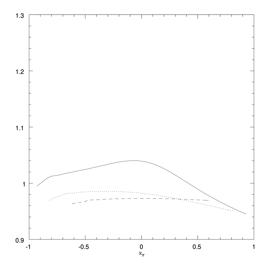
Figure 6:

Figure 7:

Figure 8:

Figure 9:

Figure 10:

Figure 11:

Figure 12:

Figure 13:

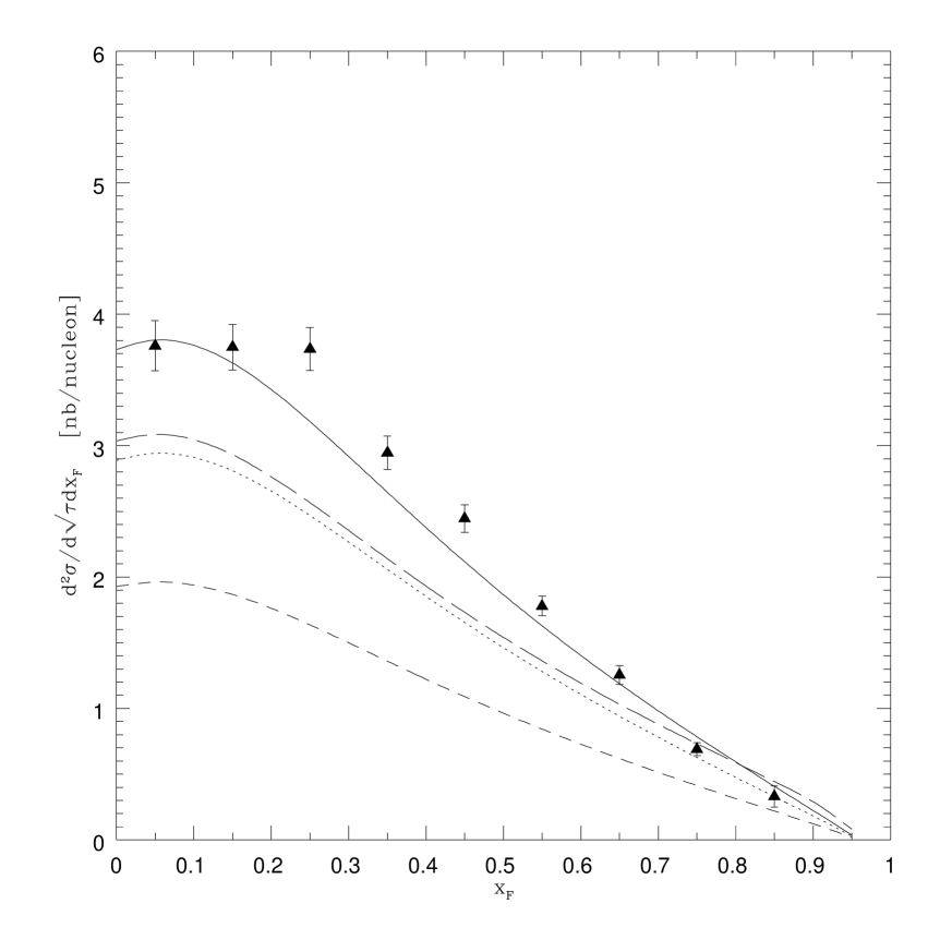
Figure 14:

Figure 15:

Figure 16:

Figure 17:

Figure 18:

Figure 19:

Figure 20:

Figure 21:

Figure 22:

References

- [1] S.D. Drell and T.M. Yan, Phys. Rev. Lett. 25 (1970) 316.
- [2] See section C of ”Heavy-ion collisions” in the proceedings of the Large Hadron Collider Workshop, Aachen, 4-9 October 1990. Editors: G. Jarlskog and D. Rein, vol III p.1057-1234.
- [3] G. Parisi, Phys. Lett. 90B (1980) 295.
- [4] G. Sterman, Nucl. Phys. 281 (1987) 310.
- [5] D. Appell, P. Mackenzie and G. Sterman, Nucl. Phys. B309 (1988) 259.
- [6] S. Catani and L. Trentadue, Nucl. Phys. B327 (1989) 323, Nucl. Phys. B353 (1991) 183.
- [7] H. Contapanagos and G. Sterman, Nucl. Phys. B419 (1994) 77.
- [8] P.M. Stevenson, Phys. Rev. D23 (1981) 2916.
- [9] G. Grunberg, Phys. Lett. 95B (1980) 70, Erratum Phys. Lett. 110B (1982) 501.
- [10] S.J. Brodsky, G.P. Lepage and P.B. Mackenzie, Phys. Rev. D28 (1983) 228.
- [11] J.H. Christenson et al., Phys. Rev. Lett. 25 (1970) 1523, Phys. Rev. D8 (1973) 2016.
-
[12]
L.M. Lederman, Phys. Rep. 26 (1976) 149;
N.S. Craigie, Phys. Rep. 47 (1978) 1. - [13] J. Badier et al. (NA3 collaboration), Phys. Lett. 89B (1979) 145
- [14] R. Barate et al. , Phys. Rev. Lett. 43 (1979) 1541.
-
[15]
G. Matthiae, Rivisita del Nuovo Cimento vol. 4, Nb.3 (1981) 1;
R. Stroynowski, Phys. Rep. 71 (1981) 1;
I.R. Kenyon, Rep. on Progr. in Phys. 45 (1982) 1261;
”Lepton pair production in hadron-hadron collisions”, by K. Freudenreich habilitation’s thesis 1988, ETH Zürich. - [16] J. Kubar-Andre and F.E. Paige, Phys. Rev. D19 (1979) 221.
- [17] G. Altarelli, R.K. Ellis and G. Martinelli, Nucl. Phys. B157 (1979) 461.
- [18] J. Kubar, M. le Bellac, J.L. Meunier and G. Plaut, Nucl. Phys. B175 (1980) 251.
- [19] B. Humpert and W.L. van Neerven, Nucl. Phys. B184 (1981) 225.
- [20] E. Anassontzis et al. (E537 collaboration), Phys. Rev. D38 (1988) 1377.
- [21] J.S. Conway et al. (E615 collaboration), Phys. Rev. D39 (1989) 92.
- [22] D.M. Alde et al. (E772 collaboration), Phys. Rev. Lett. 64 (1990) 2479.
- [23] P.L. McGaughey et al. (E772 collaboration), Phys Rev. Lett. 69 (1992) 1726.
- [24] R. Hamberg, W.L. van Neerven and T. Matsuura, Nucl. Phys. B359 (1991) 343.
- [25] W.L. van Neerven and E.B. Zijlstra, Nucl. Phys. B382 (1992) 11.
-
[26]
T. Matsuura and W.L. Neerven, Z. Phys. C38 (1988) 623;
T. Matsuura, S.C. van der Marck and W.L. van Neerven, Nucl. Phys. B319 (1989) 570, Phys. Lett. 211B (1988) 171. - [27] P. Aurenche and P. Chiappetta, Z. Phys. C34 (1987) 201.
- [28] P.J. Sutton, A.D. Martin, R.G. Roberts, W.J. Stirling, Phys. Rev. D45 (1992) 2349.
- [29] A.D. Martin, W.J. Stirling and R.G. Roberts, Phys. Rev. D47 (1993) 867, Phys. Lett. 306B (1993) 145, Erratum Phys. Lett. 309B (1993) 492.
- [30] J.F. Owens, Phys. Rev. D30 (1984) 943.
- [31] M. Glück, E. Reya, A. Vogt, Z. Phys. C53 (1992) 651.
- [32] W. Furmanski and R. Petronzio, Phys. Lett. 97B (1980) 437.
- [33] W. Furmanski and R. Petronzio, Z. Phys. C11 (1982) 293.