DESY 94-125
July 1994

SMATASY

A program for the model independent
description of the $Z$ resonance

Stefan Kirsch   and   Tord Riemann
DESY – Institut für Hochenergiephysik
Platanenallee 6, D-15738 Zeuthen, Germany

ABSTRACT
SMATASY is an interface for the ${}_{Z\!F}\!I\!^{\textstyle T}\!\!T\!\!_{{\textstyle E}\!R}$ package and may be used for the model independent description of the $Z$ resonance at LEP 1 and SLC. It allows the determination of the $\mathrm{Z}$ mass and width and its resonance shape parameters $r$ and $j$ for cross-sections and their asymmetries. The $r$ describes the peak height and $j$ the interference of the $Z$ resonance with photon exchange in each scattering channel and for $\sigma_{T}$, $\sigma_{FB}$, $\sigma_{lr}$, $\sigma_{pol}$ etc. separately. Alternatively, the helicity amplitudes for a given scattering channel may be determined. We compare our formalism with other model independent approaches. The model independent treatment of QED corrections in SMATASY is applicable also far away from the $\mathrm{Z}$ peak.

PROGRAM SUMMARY

Title of program:

SMATASY version 2.2

Catalogue number:

Program obtainable from:

CPC Program Library, Queen’s University of Belfast, N. Ireland (see application form in this issue)

Licensing provisions:

none

Computer for which the program is designed:

any computer with a FORTRAN 77 compiler

Operating system under which the program has been tested:

UNIX

Programming language used:

FORTRAN 77

Memory required to execute with typical data:

34000 words

No. of bits in a word:

32

No. of lines in distributed program, including test data, etc:

1204

Keywords:

electron–positron annihilation, scattering matrix, cross sections, asymmetries, model independent ansatz, radiative corrections

Nature of the physical problem:

The program determines cross sections and asymmetries in the vicinity of the $\mathrm{Z}$ resonance taking into account radiative corrections up to ${\cal O}(\alpha^{2})\>$. This model independent determination is based on the S-matrix approach.

Methode of solution:

SMATASY is designed as a new interface of the ZFITTER  package [3]. Therefore it relies on the same treatment of radiative corrections as ZFITTER .

LONG WRITEUP

1 Introduction

With the rising precision of the experimental study of the $Z$ resonance at LEP 1 and SLC, an interpretation of the data in a rigorously model independent way becomes more and more important. A wrong theoretical description of the data may lead to systematic non-observed shifts of the measured parameters which describe the $Z$.

SMATASY is a program for the model independent study of fermion pair production at the $\mathrm{Z}$ resonance:

$$e^{+}e^{-}\rightarrow(\gamma,Z)\rightarrow f^{+}f^{-}(n\gamma).$$ (1)

Under the assumption that QED and QCD are well understood theories, the total cross-section around the $\mathrm{Z}$ peak may be characterized by four real parameters: the mass $M_{Z}$, width $\Gamma_{Z}$, the residuum $r$ of the $Z$ resonance, and the strength of the $\gamma$$\mathrm{Z}$-interference $j$. The parameters $r$ and $j$ are related to helicity amplitudes $\mathrm{R_{Z}}^{fi}$ for $e^{+}e^{-}$ annihilation into fermion pairs via $\mathrm{Z}$-exchange. Further, the measured cross-section includes photonic virtual and real bremsstrahlung corrections which may be described by a flux function $\rho_{T}(s^{\prime}/s)$ [1]:

$$\sigma_{T}(s)=\frac{4}{3}\pi\alpha^{2}\int\frac{ds^{\prime}}{s}\left[\frac{r^{\gamma}}{s}+\frac{sr+(s-M_{Z}^{2})j}{(s-M_{Z}^{2})^{2}+M_{Z}^{2}\Gamma_{Z}^{2}}\right]\rho_{T}\left(\frac{s^{\prime}}{s}\right).$$ (2)

As mentioned, the photon exchange parameter $r^{\gamma}$ is assumed to be known, and $s$ depends on the beam energy, $s=4E^{2}$. Further, at LEP 1 and SLC very precise measurements of various cross-section asymmetries are performed. An example is shown in figure 1. In the vicinity of the $\mathrm{Z}$ peak, these asymmetries behave relatively smoothly and may be described by a simple, universal formula [2]:

$$A(s)=A_{0}+C(s)\,A_{1}\left(\frac{s}{M_{Z}^{2}}-1\right).$$ (3)

The QED corrections are contained in the factor $C(s)$.

The model independent description of cross-sections around the $\mathrm{Z}$ resonance with account of QED corrections may be done with the ${}_{Z\!F}\!I\!^{\textstyle T}\!\!T\!\!_{{\textstyle E}\!R}$ [3]–[6] branch ZUSMAT. Here, we describe the Fortran program SMATASY which is designed as an interface to ${}_{Z\!F}\!I\!^{\textstyle T}\!\!T\!\!_{{\textstyle E}\!R}$ for the model independent description of asymmetries. SMATASY provides the full functionality of ${}_{Z\!F}\!I\!^{\textstyle T}\!\!T\!\!_{{\textstyle E}\!R}$ with all its possibilities of flag settings, different treatments of photonic bremsstrahlung and QCD corrections.

SMATASY is devoted to the following tasks:

• determination of the $\mathrm{Z}$-exchange parameters $r$ and $\gamma$$\mathrm{Z}$-interference parameters $j$ for cross-sections and asymmetries,

• determination of the asymmetry parameters $A_{0}$ and $A_{1}$,

• determination of the couplings $\mathrm{R_{Z}}^{fi}$ of helicity amplitudes describing the $\mathrm{Z}$-exchange matrix element,

• model independent treatment of QED corrections for cross-sections and asymmetries.

The basic formulae are introduced in section 2 and related to other approaches in section 3. The structure of the SMATASY package is explained in section 4 while the procedures are described in section 5. Appendix A contains a sample output of SMATASY.

Figure 1: The forward-backward asymmetry for the process $e^{+}e^{-}\rightarrow\mu^{+}\mu^{-}$ near the $\mathrm{Z}$ peak.

2 Basic formulae

2.1 Cross-sections at the $\mathrm{Z}$ resonance

The matrix element for the production of a fermion pair near the $\mathrm{Z}$ resonance may be described by four helicity amplitudes. In full generality, they have the following form [1, 7]:

$${\cal M}^{fi}(s)=\frac{\mathrm{R}^{f}_{\gamma}}{s}+\frac{\mathrm{R_{Z}}^{fi}}{s-s_{Z}}+\sum_{n=0}^{\infty}\frac{\mathrm{F}_{n}^{fi}}{{\overline{M}}_{Z}^{2}}\left(\frac{s-s_{Z}}{{\overline{M}}_{Z}}\right)^{n},~{}~{}\ i=1,\ldots,4.$$ (4)

The position of the $\mathrm{Z}$ pole in the complex $s$ plane is given by $s_{\mathrm{Z}}$:

$$s_{Z}={\overline{M}}_{Z}^{2}-i{\overline{M}}_{Z}{\overline{\Gamma}}_{Z}.$$ (5)

The $\mathrm{R}^{f}_{\gamma}$ and $\mathrm{R_{Z}}^{fi}$ are complex residua of the photon and the $\mathrm{Z}$ boson, respectively. In Born approximation, they are real numbers. In the Standard Model, contributions from higher order corrections are incorporated and the residua become complex numbers. The coefficients $\mathrm{F}_{n}^{fi}$ in (4) describe nonresonant contributions to the scattering process. In the Standard Model they arise from higher order corrections, e.g. from $\mathrm{Z}$$\mathrm{Z}$ and WW box diagrams. The s dependence of the virtual electroweak corrections also contributes to them.

To a very good approximation, the Taylor series in (4) may be neglected. Its first term F${}_{0}^{fi}$ is constant. In a $\mathrm{Z}$ line shape fit, it will be strongly correlated with the photon exchange term $\mathrm{R}^{f}_{\gamma}/s\approx\mathrm{R}^{f}_{\gamma}/{\overline{M}}_{Z}^{2}$,

$$\mathrm{R}^{f}_{\gamma}=\displaystyle{F_{A}(s)\left|Q_{e}Q_{f}\right|}.$$ (6)

The $Q_{f}$ is the electric charge of the final state fermions and $F_{A}(s)$ the vacuum polarization of the photon:

$$F_{A}({\overline{M}}_{Z}^{2})=\displaystyle{\frac{\alpha({\overline{M}}_{Z}^{2})}{\alpha}}=\frac{137.06}{128.86}-i\,0.0188.$$ (7)

In practice it seems to be impossible to disentangle $F_{A}$ and the nonresonating quantum correction F${}_{0}^{fi}$. The next-to-leading background term is proportional to $\sigma=(s-s_{Z})/{\overline{M}}_{Z}^{2}\approx 2(\sqrt{s}/{\overline{M}}_{Z}-1)$. At LEP 1 and SLC the bulk of data is taken at $|\sqrt{s}-{\overline{M}}_{Z}|<{\overline{\Gamma}}_{Z}$ and $\sigma$ becomes less than 5 %. Having in mind that the $F_{n}^{fi}$ are quantum corrections and proportional to $\alpha/\pi$, it is for all practical needs:

$${\cal M}^{fi}(s) = \frac{\mathrm{R}^{f}_{\gamma}}{s}+\frac{\mathrm{R_{Z}}^{fi}}{s-s_{Z}}+\frac{F_{0}^{fi}}{{\overline{M}}_{Z}}$$ (8)

$$\approx ~{}\frac{\mathrm{R}^{f}_{\gamma}}{s}+\frac{\mathrm{R_{Z}}^{fi}}{s-s_{Z}}.$$

There are four residua $\mathrm{R_{Z}}^{fi}$ for the four independent helicity amplitudes in the case of massless external fermions:

$$\begin{array}[]{lcl}R_{Z}^{f0}&=&R_{Z}(e^{-}_{L}e^{+}_{R}\longrightarrow f^{-}_{L}f^{+}_{R}),\\ R_{Z}^{f1}&=&R_{Z}(e^{-}_{L}e^{+}_{R}\longrightarrow f^{-}_{R}f^{+}_{L}),\\ R_{Z}^{f2}&=&R_{Z}(e^{-}_{R}e^{+}_{L}\longrightarrow f^{-}_{R}f^{+}_{L}),\\ R_{Z}^{f3}&=&R_{Z}(e^{-}_{R}e^{+}_{L}\longrightarrow f^{-}_{L}f^{+}_{R}).\end{array}$$ (13)

The amplitudes ${\cal M}^{fi}(s)$ give rise to four cross-sections $\sigma_{i}$ which add up incoherently to the following measurable cross-sections:

$$\begin{array}[]{lclcl}&&\sigma_{T}^{0}(s)&=&+~{}\sigma_{0}+\sigma_{1}+\sigma_{2}+\sigma_{3},\\ \sigma_{\mbox{\scriptsize\it lr-pol}}^{0}(s)&=&\sigma_{FB}^{0}(s)&=&+~{}\sigma_{0}-\sigma_{1}+\sigma_{2}-\sigma_{3},\\ \sigma_{\mbox{\scriptsize\it FB-lr}}^{0}(s)&=&\sigma_{pol}^{0}(s)&=&-~{}\sigma_{0}+\sigma_{1}+\sigma_{2}-\sigma_{3},\\ \sigma_{lr}^{0}(s)&=&\sigma_{\mbox{\scriptsize\it FB-pol}}^{0}(s)&=&-~{}\sigma_{0}-\sigma_{1}+\sigma_{2}+\sigma_{3}.\end{array}$$ (18)

Here, the $\sigma_{T}^{0}$ is the total cross-section, $\sigma_{FB}^{0}$ defines the forward-backward asymmetry, $\sigma_{pol}^{0}$ the final state polarization, $\sigma_{FB,pol}^{0}$ the forward-backward asymmetry of the final state polarization etc.

All these cross-sections may be parameterized by the following master formula [1]:

$$\sigma_{A}^{0}(s) = \displaystyle{\frac{4}{3}\pi\alpha^{2}\left[\frac{r^{\gamma f}_{A}}{s}+\frac{sr^{f}_{A}+(s-{\overline{M}}_{Z}^{2})j^{f}_{A}}{(s-{\overline{M}}_{Z}^{2})^{2}+{\overline{M}}_{Z}^{2}{\overline{\Gamma}}_{Z}^{2}}+\frac{r_{A}^{f0}}{{\overline{M}}_{Z}^{2}}\right]},\hskip 14.22636ptA=\mbox{\it T, FB, pol, FB-pol,}\ldots$$ (19)

$$\approx \displaystyle{\frac{4}{3}\pi\alpha^{2}\left[\frac{r^{\gamma f}_{A}}{s}+\frac{sr^{f}_{A}+(s-{\overline{M}}_{Z}^{2})j^{f}_{A}}{(s-{\overline{M}}_{Z}^{2})^{2}+{\overline{M}}_{Z}^{2}{\overline{\Gamma}}_{Z}^{2}}\right]}.$$

The $r^{\gamma f}_{A}$ is the photon exchange term,

$$r^{\gamma f}_{A}=\displaystyle{\frac{1}{4}c_{f}\sum_{i=0}^{3}\{\pm 1\}\left|\mathrm{R}^{f}_{\gamma}\right|^{2}}R_{QCD},$$ (20)

vanishes for all asymmetric cross-sections. $c_{f}=1,3$ for leptons and quarks, respectively. QCD corrections for quarks are taken into account by the factor $R_{QCD}$ of [3]. The $\mathrm{Z}$-exchange residuum $r^{f}_{A}$ and the $\gamma$$\mathrm{Z}$-interference $j^{f}_{A}$ are:

$$\begin{array}[]{lll}r^{f}_{A}&=&\displaystyle{c_{f}\left\{\frac{1}{4}\sum_{i=0}^{3}\{\pm 1\}\left|\mathrm{R_{Z}}^{fi}\right|^{2}+2\frac{{\overline{\Gamma}}_{Z}}{{\overline{M}}_{Z}}\mbox{$\Im$m}C^{f}_{A}\right\}}R_{QCD},\\ j^{f}_{A}&=&c_{f}\left\{2\mbox{$\Re$e}C^{f}_{A}-2\displaystyle{\frac{{\overline{\Gamma}}_{Z}}{{\overline{M}}_{Z}}}\mbox{$\Im$m}C^{f}_{A}\right\}R_{QCD},\\ C^{f}_{A}&=&(R^{f}_{\gamma})^{*}\left(\displaystyle{\frac{1}{4}\sum_{i=0}^{3}\{\pm 1\}\mathrm{R_{Z}}^{fi}}\right).\end{array}$$ (24)

The factors $\{\pm 1\}$ in (20) and (24) indicate that the signs of $\left|R_{\gamma}^{f}\right|$, $\left|\mathrm{R_{Z}}^{fi}\right|^{2}$, and of $\mathrm{R_{Z}}^{fi}$ correspond to the signs of $\sigma_{i}$ in (18).

2.2 QED corrections for cross-sections

For the calculation of QED corrections in SMATASY the ${}_{Z\!F}\!I\!^{\textstyle T}\!\!T\!\!_{{\textstyle E}\!R}$ environment is used. This is done by convoluting (19) with radiator functions for initial and final state radiation and their interference. The initial and final state corrections with soft photon exponentiation to the cross-sections $\sigma_{T}$, $\sigma_{\mathrm{pol}}$, $\sigma_{lr}$, $\sigma_{\mbox{\scriptsize\it lr-pol}}$  are described by:

$$\sigma_{A}(s)=\int\frac{ds^{\prime}}{s}\sigma_{A}^{0}(s^{\prime})\rho_{T}\left(\frac{s^{\prime}}{s}\right)\hskip 14.22636ptA=\mbox{\it T, pol, lr, lr-pol}.$$ (25)

Analogously, for the forward-backward difference cross-sections,

$$\sigma_{a}(s)=\int\frac{ds^{\prime}}{s}\sigma_{a}^{0}(s^{\prime})\rho_{FB}\left(\frac{s^{\prime}}{s}\right),\hskip 14.22636pta=\mbox{\it FB, FB-pol, FB-lr.}$$ (26)

We stress that $\rho_{FB}(s^{\prime}/s)\neq\rho_{T}(s^{\prime}/s)$. The contributions from initial final state interference bremsstrahlung are slightly more complex [3]–[6]. At the $\mathrm{Z}$ resonance they are numerically tiny as long as no strong cuts are applied. They will be neglected in the following. With QED corrections, the master formula may be rewritten as follows  [2]:

$${\bar{\sigma}}_{A}(s) = \frac{4}{3}\pi\alpha^{2}\left[\frac{{\bar{r}}^{\gamma f}_{A}}{s}+\frac{s{\bar{r}}_{A}^{f}+(s-{\overline{M}}_{Z}^{2}){\bar{j}}_{A}^{f}}{(s-{\overline{M}}_{Z}^{2})^{2}+{\overline{M}}_{Z}^{2}{\overline{\Gamma}}_{Z}^{2}}+\frac{{\bar{r}}_{A}^{0f}}{M_{Z}^{2}}\right]$$ (27)

$$\approx ~{}\frac{4}{3}\pi\alpha^{2}\left[\frac{{\bar{r}}^{\gamma f}_{A}}{s}+\frac{s{\bar{r}}_{A}^{f}+(s-{\overline{M}}_{Z}^{2}){\bar{j}}_{A}^{f}}{(s-{\overline{M}}_{Z}^{2})^{2}+{\overline{M}}_{Z}^{2}{\overline{\Gamma}}_{Z}^{2}}\right].$$

The barred parameters contain correction factors with QED corrections:

$$\begin{array}[]{lcl}{\bar{r}}_{T}^{\gamma f}&=&C^{\gamma}_{T}(s)\,\,r_{T}^{\gamma f},\\ {\bar{r}}_{A}^{f}&=&C^{r}_{A}(s)\,\,r_{A}^{f},\\ {\bar{j}}_{A}^{f}&=&C^{j}_{A}(s)\,\,j_{A}^{f},\\ {\bar{r}}_{A}^{0f}&=&C_{A}^{0}(s)\,\,r_{A}^{0f},\end{array}$$ (32)

where

$$\begin{array}[]{lcl}C^{\gamma}_{T}(s)&=&\displaystyle{{\cal I}\left[\frac{s}{s^{\prime}}\right]},\\ C_{A}^{r}(s)&=&\displaystyle{{\cal I}\left[\frac{s^{\prime}}{s}\,\,\frac{(s-{\overline{M}}_{Z}^{2})^{2}+{\overline{M}}_{Z}^{2}{\overline{\Gamma}}_{Z}^{2}}{(s^{\prime}-{\overline{M}}_{Z}^{2})^{2}+{\overline{M}}_{Z}^{2}{\overline{\Gamma}}_{Z}^{2}}\right]},\\ C_{A}^{j}(s)&=&\displaystyle{{\cal I}\left[\frac{s^{\prime}-{\overline{M}}_{Z}^{2}}{s-{\overline{M}}_{Z}^{2}}\,\,\frac{(s-{\overline{M}}_{Z}^{2})^{2}+{\overline{M}}_{Z}^{2}{\overline{\Gamma}}_{Z}^{2}}{(s^{\prime}-{\overline{M}}_{Z}^{2})^{2}+{\overline{M}}_{Z}^{2}{\overline{\Gamma}}_{Z}^{2}}\right]},\\ C_{A}^{0}(s)&=&\displaystyle{{\cal I}\left[\frac{(s^{\prime}-{\overline{M}}_{Z}^{2})^{0}}{(s-{\overline{M}}_{Z}^{2})^{0}}\right]}={\cal I}\left[1\right].\end{array}$$ (37)

Here, the definition

$${\cal I}_{A}[B]=\int d\left(\frac{s^{\prime}}{s}\right)B(s^{\prime})\rho_{A}\left(\frac{s^{\prime}}{s}\right)$$ (38)

is used. The QED correction factors are completely model independent, i.e. independent of the underlying dynamics of the scattering process. They depend on mass and width of the $\mathrm{Z}$ and on the handling of the photonic phase space, the inclusion of higher orders, and on acceptance cuts. The reader may wonder that the corrections $C_{A}^{j}$ seem to be singular at $\sqrt{s}={\overline{M}}_{Z}.$ This is not the case for the products $C_{A}^{j}(s)(s-{\overline{M}}_{Z})$ which are physically relevant. As may be seen from the corresponding definitions, these products remain small (but potentially non-vanishing) when $\sqrt{s}$ approaches ${\overline{M}}_{Z}$. There the QED corrected cross-sections may be defined as (smooth) limits from the neighboring energies.

The correction factors are shown in figures 2–4 without and with two different cuts on the photon phase space. All QED corrections are smooth and, with one exception, rather independent of $s$. Those to the $\mathrm{Z}$ exchange, $C_{A}^{r}$, develop the radiative tail at the right hand side of the peak which at some value of $s$ gets suppressed by the cuts. It may be further seen that the corrections to total cross-sections and those to forward-backward differences are not equal, although of similar size near the peak. They deviate more when more hard bremsstrahlung is possible [6]. This explains the rise of their difference with the tail and the subsequent vanishing of it after the cuts become influential.

2.3 Asymmetries around the $\mathrm{Z}$ resonance

Without QED corrections, asymmetries are defined by:

$${\cal A}_{A}^{0}(s)=\frac{\sigma_{A}^{0}(s)}{\sigma_{T}^{0}(s)},~{}~{}~{}A\neq T.$$ (39)

These asymmetries take an extremely simple form around the $\mathrm{Z}$ resonance [2]:

$${\cal A}_{A}^{0}(s)=A_{0}^{A}+A_{1}^{A}\left(\frac{s}{{\overline{M}}_{Z}^{2}}-1\right)+A_{2}^{A}\left(\frac{s}{{\overline{M}}_{Z}^{2}}-1\right)^{2}+\ldots\approx A_{0}^{A}+A_{1}^{A}\left(\frac{s}{{\overline{M}}_{Z}^{2}}-1\right).$$ (40)

Figure 2: The model independent QED correction factors without cuts.

Figure 3: The model independent QED correction factors with a cut on the energy of the bremsstrahlung photon.

Figure 4: The model independent QED correction factors with cuts on the acollinearity $\xi$ of the final state fermions and on their energy $E_{f}$.

The higher order terms may be safely neglected since $(s/{\overline{M}}_{Z}^{2}-1)^{2}=\sigma^{2}<2\times 10^{-4}$. The coefficients have a quite simple form:

$$A_{0}^{A} = \frac{r_{A}^{f}}{r_{T}^{f}+\gamma^{2}r^{\gamma f}_{T}}\approx\frac{r_{A}^{f}}{r_{T}^{f}},$$ (41)

$$A_{1}^{A} = \left[\frac{j^{f}_{A}}{r_{A}^{f}}-\frac{j_{T}^{f}-2\gamma^{2}r^{\gamma f}_{T}}{r_{T}^{f}+\gamma^{2}r^{\gamma f}_{T}}\right]A_{0}^{A}\approx\left[\frac{j^{f}_{A}}{r_{A}^{f}}-\frac{j_{T}^{f}}{r_{T}^{f}}\right]A_{0}^{A}.$$ (42)

Here, the $r_{A}^{0f}$ is neglected in both $A_{0}$ and $A_{1}$. Further, the definition $\gamma^{2}={\overline{\Gamma}}_{Z}^{2}/{\overline{M}}_{Z}^{2}\approx 0.75\times 10^{-3}$ is used.

2.4 QED corrections for asymmetries

A typical cross-section asymmetry with QED corrections is shown in figure 1. The Born asymmetry is linear around the $\mathrm{Z}$ resonance. QED corrections lead to deviations from this; specially pronounced at the right hand side of the peak. Although asymmetries get much smaller QED corrections than the cross-sections themselves, an analysis of the data would not be consistent without their correct treatment.

With QED corrections, the master formula for asymmetries becomes:

$${\bar{\cal A}}_{A}(s) = {\bar{A}}_{0}^{A}+{\bar{A}}_{1}^{A}\left(\frac{s}{{\overline{M}}_{Z}^{2}}-1\right).$$ (43)

The coefficients ${\bar{A}}_{n}$ may be obtained from the $A_{n}$ defined in section 2.3 by replacing in their definitions the unbarred variables by barred ones.

For the peak contributions to the forward-backward asymmetries the explicit expressions are:

$${\bar{A}}_{0}^{a} = \frac{C_{FB}^{r}}{C_{T}^{r}}\frac{r_{a}^{f}}{r_{T}^{f}+[C_{T}^{\gamma}/C_{T}^{r}]\gamma^{2}r^{\gamma f}_{T}}$$ (44)

$$\approx \frac{C_{FB}^{r}}{C_{T}^{r}}\frac{r_{a}^{f}}{r_{T}^{f}+0.001}$$

$$\approx 0.998\frac{r_{a}^{f}}{r_{T}^{f}+0.001}\approx\frac{r_{a}^{f}}{r_{T}^{f}},\hskip 14.22636pta=\mbox{\it FB, FB-pol, FB-lr.}$$

Aiming at an experimental accuracy of $\Delta{\cal A}_{FB}^{lep}=0.001$ at LEP 1, the deviation of $C_{FB}^{r}/C_{T}^{r}$ from unity has to be taken into account. Compared to ${\cal A}_{FB}$, ${\cal A}_{\mbox{\scriptsize\it FB-pol}}$ and ${\cal A}_{\mbox{\scriptsize\it FB-lr}}$ the expressions for ${\cal A}_{pol}$, ${\cal A}_{lr}$ and ${\cal A}_{\mbox{\scriptsize\it lr-pol}}$ are simpler since the QED corrections to the numerator and the denominator are both of the total cross-section type. The leading term is:

$${\bar{A}}_{0}^{A} = \frac{r_{A}^{f}}{r_{T}^{f}+[C_{T}^{\gamma}/C^{r}_{T}]\gamma^{2}r_{T}^{\gamma f}}$$ (45)

$$\approx \frac{r_{A}^{f}}{r_{T}^{f}+0.001}\approx\frac{r_{A}^{f}}{r_{T}^{f}},\hskip 14.22636ptA=\mbox{\it pol, lr, lr-pol}.$$

The coefficients $\bar{A}_{1}^{A}$ are in reasonable approximation:

$${\bar{A}_{1}^{a}} = C(s)\left[\frac{C_{FB}^{j}}{C_{T}^{j}}\frac{C_{T}^{r}}{C_{FB}^{r}}\frac{j_{a}^{f}}{r_{a}^{f}}-\frac{j_{T}^{f}}{r_{T}^{f}}\right]{\bar{A}_{0}^{a}}$$ (46)

$$\approx C(s)\left[\frac{j_{a}^{f}}{r_{a}^{f}}-\frac{j_{T}^{f}}{r_{T}^{f}}\right]{\bar{A}_{0}^{a}},\hskip 14.22636pta=\mbox{\it FB, FB-pol, FB-lr,}$$

$$\bar{A}_{1}^{A} = C(s)\left[\frac{j_{A}^{f}}{r_{A}^{f}}-\frac{j_{T}^{f}}{r_{T}^{f}}\right]{\bar{A}_{0}^{A}},\hskip 14.22636ptA=\mbox{\it pol, lr, lr-pol}.$$ (47)

The coefficients with a pronounced $s$ dependence are

$$C(s)\equiv C_{T}(s)=\frac{C^{j}_{T}}{C^{r}_{T}},\hskip 19.91684ptC_{FB}(s)=\frac{C^{j}_{FB}}{C^{r}_{FB}}\approx C(s).$$ (48)

The behaviour of $C_{T}$ and $C_{FB}$ as functions of $s$ and the dependence on cuts is shown in figure 5. As mentioned already, the $C_{T}(s/{\overline{M}}_{Z}^{2}-1)$ does not vanish at $\sqrt{s}={\overline{M}}_{Z}$ but is extremely small. Aiming at an accuracy of several per mill, one may neglect the difference between $C_{T}$ and $C_{FB}$ in the vicinity of the peak. The initial state QED corrections to the $\mathrm{Z}$-exchange cross-section develop a radiative tail while those to the $\gamma$$\mathrm{Z}$-interference do not. Due to this, their ratio $C(s)$ gets damped at the right hand side of the $\mathrm{Z}$ peak. This damping was seen in figure 1. It may be assigned to QED corrections completely. At $\sqrt{s}>{\overline{M}}_{Z}$, the radiative tail may be avoided by a cut on the energy of the emitted photons:

$$\frac{E_{\gamma}}{E_{\mathrm{beam}}}<\Delta=1-\frac{M_{Z}^{2}}{s}.$$ (49)

At LEP 1 and SLC, where $\sqrt{s}\approx{\overline{M}}_{Z}$, this condition is rather restrictive; e.g. at $\sqrt{s}={\overline{M}}_{Z}+2{\overline{\Gamma}}_{Z}$, it is $\Delta=0.1$. In figures 1 and 5, photons are cut with energies larger than 6 GeV. The radiative tail is suppressed by this if $\sqrt{s^{\prime}}>{\overline{M}}_{Z}$ is ensured. At $\sqrt{s}>{\overline{M}}_{Z}/\sqrt{1-E_{\gamma}/E_{\mathrm{beam}}}=97.5$ GeV this is the case. In the immediate vicinity of the peak one unavoidably measures data which contain radiative corrections. As may be seen from the figure, the other cuts (on the acollinearity and energy of the final state fermions) are similar [3].

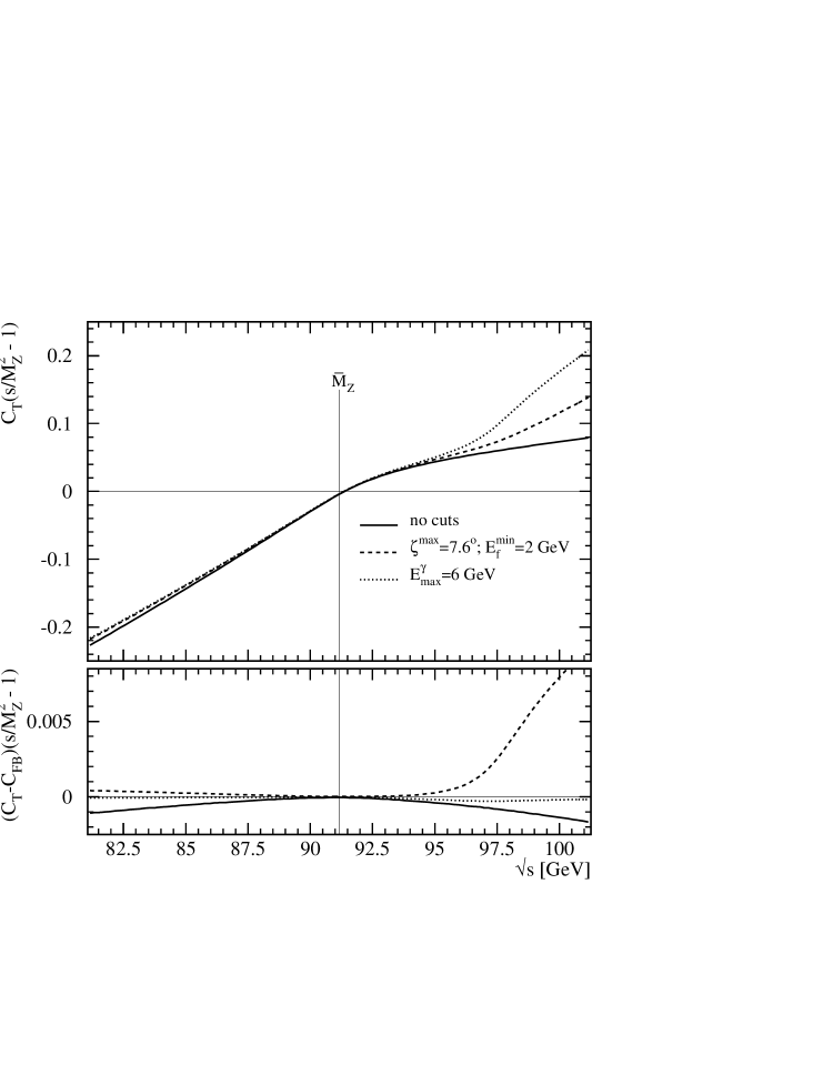
Figure 5: The model independent QED correction to the slope of asymmetries near the $\mathrm{Z}$ peak.

3 Other model independent approaches

3.1 The BCMS approach

In [8, 9] the following model independent formula for the total cross-section has been advocated:

$${\sigma_{T}^{o}(s)=\frac{12\pi\Gamma_{e}\Gamma_{f}}{\left|s-s_{0}\right|^{2}}\left\{\frac{s}{M_{Z}^{2}}+{\cal R}_{f}\frac{s-M_{Z}^{2}}{M_{Z}^{2}}+{\cal I}_{f}\frac{\Gamma_{Z}}{M_{Z}}+\ldots\right\}+\sigma_{\mathrm{QED}}^{f}.}$$ (50)

The free parameters of the above expression may be calculated within the Standard Model with account of electroweak radiative corrections  [8, 10]. There is a simple one–to–one correspondence to the parameters in (19) [3]:

$$r_{T}^{f} = \frac{9}{\alpha^{2}}\frac{\Gamma_{e}\Gamma_{f}}{M_{Z}^{2}}\left(1+\frac{\Gamma_{Z}}{M_{Z}}{\cal I}_{f}\right),$$

$$j_{T}^{f} = \frac{9}{\alpha^{2}}\frac{\Gamma_{e}\Gamma_{f}}{M_{Z}^{2}}\left({\cal R}_{f}-\frac{\Gamma_{Z}}{M_{Z}}{\cal I}_{f}\right),$$ (51)

$$-2\left|Q_{e}Q_{f}\right|\frac{\sum\mathrm{R_{Z}}^{fi}}{\sum|\mathrm{R_{Z}}^{fi}|^{2}}\Im mF_{A} = {\cal I}_{f}.$$

Further,

$$s_{0}=M_{Z}^{2}-i\frac{s}{M_{Z}}\Gamma_{Z}.$$ (52)

The relation between the definitions of $s_{0}$ and $s_{Z}$ is given to a very good approximation by the following equalities, which also affect the coupling strength [11]:

$$\begin{array}[]{lllllcr}{\overline{M}}_{Z}&=&[1+(\Gamma_{\mathrm{Z}}/M_{Z})^{2}]^{-\frac{1}{2}}M_{Z}&\approx&M_{Z}&-&34~{}{\hbox{\rm\ Me\kern-1.00006ptV}},\\ {\overline{\Gamma}}_{\mathrm{Z}}&=&[1+(\Gamma_{\mathrm{Z}}/M_{Z})^{2}]^{-\frac{1}{2}}\Gamma_{\mathrm{Z}}&\approx&\Gamma_{\mathrm{Z}}&-&1~{}{\hbox{\rm\ Me\kern-1.00006ptV}},\\ \overline{\mathrm{G}}_{\mu}&=&\mathrm{G}_{\mu}/(1+i\Gamma_{\mathrm{Z}}/MZ).&&\end{array}$$ (56)

3.2 The OPAL approach

A completely different approach has been chosen in [12]. With an ad hoc ansatz, the effective couplings of the differential cross-section have been allowed to deviate from what is expected in the Standard Model in the approximation of effective fermion couplings:

$$\frac{2s}{\pi\alpha^{2}}\frac{d\sigma}{d\cos\vartheta} = \left(1+\cos\vartheta^{2}\right)\left\{\left|F_{A}\right|^{2}+8\Re e\left[F_{A}^{*}\chi(s)\right]{\cal C}_{\gamma Z}^{s}+16\left|\chi(s)\right|^{2}{\cal C}_{ZZ}^{s}\right\}$$ (57)

$$+~{}2\cos\vartheta\left\{8\Re e\left[F_{A}^{*}\chi(s)\right]{\cal C}_{\gamma Z}^{a}+64\left|\chi(s)\right|^{2}{\cal C}_{ZZ}^{a}\right\},$$

with

$$\chi(s) = \kappa\frac{s}{(s-M_{Z}^{2})^{2}+(M_{Z}\Gamma_{Z}/s)^{2}},$$ (58)

$$\kappa = \frac{G_{\mu}M_{Z}^{2}}{\sqrt{2}2\pi\alpha},$$ (59)

and

$$\begin{array}[]{lcl}{\cal C}_{ZZ}^{s}&=&\displaystyle{\frac{1}{16}\kappa_{ZZ}^{s}\left[(\hat{g}_{\mathrm{A}}^{\mathrm{e}})^{2}+(\hat{g}_{\mathrm{V}}^{\mathrm{e}})^{2}\right]\left[(\hat{g}_{\mathrm{A}}^{f})^{2}+(\hat{g}_{\mathrm{V}}^{f})^{2}\right]},\\ {\cal C}_{\gamma Z}^{s}&=&\displaystyle{\frac{1}{4}\kappa_{\gamma Z}^{s}\hat{g}_{\mathrm{V}}^{\mathrm{e}}\hat{g}_{\mathrm{V}}^{f}},\\ {\cal C}_{ZZ}^{a}&=&\displaystyle{\frac{1}{16}\kappa_{ZZ}^{a}\hat{g}_{\mathrm{A}}^{\mathrm{e}}\hat{g}_{\mathrm{V}}^{\mathrm{e}}\hat{g}_{\mathrm{A}}^{f}\hat{g}_{\mathrm{V}}^{f}},\\ {\cal C}_{\gamma Z}^{a}&=&\displaystyle{\frac{1}{4}\kappa_{\gamma Z}^{a}\hat{g}_{\mathrm{A}}^{\mathrm{e}}\hat{g}_{\mathrm{A}}^{f}}.\end{array}$$ (64)

Here, the definitions

$$\begin{array}[]{lcl}\hat{g}_{\mathrm{A}}^{f}&=&\sqrt{\rho}/2,\\ \hat{g}_{\mathrm{V}}^{f}&=&\hat{g}_{\mathrm{A}}^{f}(1-4|Q_{f}|s_{W}^{2eff}),\end{array}$$ (67)

are used for the effective couplings in the Standard Model. The parameters $\kappa$ in the definitions of the parameters $\cal C$ allow for deviations of the cross-sections and asymmetries from the Standard Model predictions where they are equal to one.

The OPAL approach uses the ${}_{Z\!F}\!I\!^{\textstyle T}\!\!T\!\!_{{\textstyle E}\!R}$ environment with minor modifications.

Up to tiny terms which are presumably much smaller than the experimental accuracy (e.g. the parameter $r_{T}^{0f}$ in the S-matrix approach), the OPAL approach is equivalent to the one advocated here. For the total cross-section and the forward-backward asymmetry the relations are:

$$\begin{array}[]{lcl}r_{T}^{f}&=&\displaystyle{16\kappa^{2}{\cal C}_{ZZ}^{s}-8\kappa\frac{\Gamma_{Z}}{M_{Z}}\Im mF_{A}{\cal C}_{\gamma Z}^{s}},\\ j_{T}^{f}&=&\displaystyle{8\kappa{\cal C}_{\gamma Z}^{s}\left[\Re eF_{A}+\frac{\Gamma_{Z}}{M_{Z}}\Im mF_{A}\right]},\\ r_{FB}^{f}&=&\displaystyle{\frac{3}{4}\left\{64\kappa^{2}{\cal C}_{ZZ}^{a}-8\kappa\frac{\Gamma_{Z}}{M_{Z}}\Im mF_{A}{\cal C}_{\gamma Z}^{a}\right\}},\\ j_{FB}^{f}&=&\displaystyle{\frac{3}{4}\left\{8\kappa{\cal C}_{\gamma Z}^{a}\left[\Re eF_{A}+\frac{\Gamma_{Z}}{M_{Z}}\Im mF_{A}\right]\right\}}.\end{array}$$ (72)

The additional factors of $\frac{3}{4}$ in the last two relations are due to the different angular integrations over even or odd integrands with respect to $\cos\vartheta$.

3.3 Effective couplings

Now we define the relation of the model independent approach of SMATASY to the use of effective weak neutral fermion couplings. The latter is realized in the ${}_{Z\!F}\!I\!^{\textstyle T}\!\!T\!\!_{{\textstyle E}\!R}$ branch ZUXSA.

In a simple quantum mechanical interpretation or an approximate quantum field theoretical one, the (complex) residua of the helicity amplitudes $\mathrm{R_{Z}}^{fi}$ may be expressed in terms of effective vector and axial vector couplings of the $\mathrm{Z}$ boson to fermions (which are basically real numbers):

$$\begin{array}[]{lcl}\mathrm{R_{Z}}^{f0}&=&\kappa(\hat{g}_{\mathrm{V}}^{\mathrm{e}}+\hat{g}_{\mathrm{A}}^{\mathrm{e}})(\hat{g}_{\mathrm{V}}^{f}+\hat{g}_{\mathrm{A}}^{f}),\\ \mathrm{R_{Z}}^{f1}&=&\kappa(\hat{g}_{\mathrm{V}}^{\mathrm{e}}+\hat{g}_{\mathrm{A}}^{\mathrm{e}})(\hat{g}_{\mathrm{V}}^{f}-\hat{g}_{\mathrm{A}}^{f}),\\ \mathrm{R_{Z}}^{f2}&=&\kappa(\hat{g}_{\mathrm{V}}^{\mathrm{e}}-\hat{g}_{\mathrm{A}}^{\mathrm{e}})(\hat{g}_{\mathrm{V}}^{f}-\hat{g}_{\mathrm{A}}^{f}),\\ \mathrm{R_{Z}}^{f3}&=&\kappa(\hat{g}_{\mathrm{V}}^{\mathrm{e}}-\hat{g}_{\mathrm{A}}^{\mathrm{e}})(\hat{g}_{\mathrm{V}}^{f}+\hat{g}_{\mathrm{A}}^{f}),\end{array}$$ (77)

with the $\kappa$ of (59) and the couplings $\hat{g}_{\mathrm{A}}^{f}$ and $\hat{g}_{\mathrm{V}}^{f}$ of (67). The parameters $r^{f}_{A}$ and $j^{f}_{A}$ of (19) are:

$$\begin{array}[]{lclcclcl}&&r^{f}_{T}&=&&\displaystyle{\kappa^{2}\left[(\hat{g}_{\mathrm{A}}^{\mathrm{e}})^{2}+(\hat{g}_{\mathrm{V}}^{\mathrm{e}})^{2}\right]\left[(\hat{g}_{\mathrm{A}}^{f})^{2}+(\hat{g}_{\mathrm{V}}^{f})^{2}\right]}&-&2\kappa\hat{g}_{\mathrm{V}}^{\mathrm{e}}\hat{g}_{\mathrm{V}}^{f}C_{Im},\\ r^{f}_{\mbox{\scriptsize\it lr-pol}}&=&\displaystyle{\frac{4}{3}}r^{f}_{FB}&=&&4\kappa^{2}\hat{g}_{\mathrm{A}}^{\mathrm{e}}\hat{g}_{\mathrm{V}}^{\mathrm{e}}\hat{g}_{\mathrm{A}}^{f}\hat{g}_{\mathrm{V}}^{f}&-&\displaystyle{2\kappa\hat{g}_{\mathrm{A}}^{\mathrm{e}}\hat{g}_{\mathrm{A}}^{f}C_{Im}},\\ \displaystyle{\frac{4}{3}}r^{f}_{\mbox{\scriptsize\it FB-lr}}&=&r^{f}_{pol}&=&-&\displaystyle{2\kappa^{2}\left[(\hat{g}_{\mathrm{A}}^{\mathrm{e}})^{2}+(\hat{g}_{\mathrm{V}}^{\mathrm{e}})^{2}\right]\hat{g}_{\mathrm{A}}^{f}\hat{g}_{\mathrm{V}}^{f}}&+&\displaystyle{2\kappa\hat{g}_{\mathrm{V}}^{\mathrm{e}}\hat{g}_{\mathrm{A}}^{f}C_{Im}},\\ r^{f}_{lr}&=&\displaystyle{\frac{4}{3}}r^{f}_{\mbox{\scriptsize\it FB-pol}}&=&-&\displaystyle{2\kappa^{2}\hat{g}_{\mathrm{A}}^{\mathrm{e}}\hat{g}_{\mathrm{V}}^{\mathrm{e}}\left[(\hat{g}_{\mathrm{A}}^{f})^{2}+(\hat{g}_{\mathrm{V}}^{f})^{2}\right]}&+&\displaystyle{2\kappa\hat{g}_{\mathrm{A}}^{\mathrm{e}}\hat{g}_{\mathrm{V}}^{f}C_{Im}},\\ \end{array}$$ (82)

and

$$\begin{array}[]{lclcclcl}&&j^{f}_{T}&=&&2\kappa\hat{g}_{\mathrm{V}}^{\mathrm{e}}\hat{g}_{\mathrm{V}}^{f}(C_{Re}+C_{Im}),&&\\ j^{f}_{\mbox{\scriptsize\it lr-pol}}&=&\displaystyle{\frac{4}{3}}j^{f}_{FB}&=&&\displaystyle{2\kappa\hat{g}_{\mathrm{A}}^{\mathrm{e}}\hat{g}_{\mathrm{A}}^{f}(C_{Re}+C_{Im})},&&\\ \displaystyle{\frac{4}{3}}j^{f}_{\mbox{\scriptsize\it FB-lr}}&=&j^{f}_{pol}&=&-&2\kappa\hat{g}_{\mathrm{V}}^{\mathrm{e}}\hat{g}_{\mathrm{A}}^{f}(C_{Re}+C_{Im}),&&\\ j^{f}_{lr}&=&\displaystyle{\frac{4}{3}}j^{f}_{\mbox{\scriptsize\it FB-pol}}&=&-&\displaystyle{2\kappa\hat{g}_{\mathrm{A}}^{\mathrm{e}}\hat{g}_{\mathrm{V}}^{f}(C_{Re}+C_{Im})}.&&\end{array}$$ (87)

Additional factors of $(3/4)^{\pm 1}$ are again due to the different angular integrations for contributions which are even or odd in $\cos\vartheta$.

The $\gamma$$\mathrm{Z}$-interference is proportional to $C_{Re}$, while $C_{Im}$ are small corrections to it and to the resonance peak parameter:

$$\begin{array}[]{lcl}C_{Im}&=&\displaystyle{\mid Q_{e}Q_{f}\mid\frac{\Gamma_{\mathrm{Z}}}{M_{Z}}\mbox{$\Im$m}F_{A}(s)},\\ C_{Re}&=&\displaystyle{\mid Q_{e}Q_{f}\mid\mbox{$\Re$e}F_{A}(s)}.\\ \end{array}$$ (90)

3.4 Model independent QED corrections

The QED correction factors in SMATASY are universal in the sense that they may be used also at energies far away from the $\mathrm{Z}$ peak and in other approaches. We give here one instructive example for this. In [13], the QED corrections to the total cross-section $\sigma_{T}(s)$ and the integrated forward-backward asymmetry have been calculated analytically without cuts to order ${\cal O}(\alpha)$ for reaction (1). The $\mathrm{Z}$ exchange cross-section contribution has been presented there as follows:

$$\sigma_{T}^{Z}(s)=\frac{4\pi\alpha^{2}}{3s}\left|\chi(s)\right|^{2}\left(v_{e}^{2}+a_{e}^{2}\right)\left(v_{f}^{2}+a_{f}^{2}\right)\left[1+\frac{\alpha}{\pi}\left(Q_{e}^{2}\,{\cal H}_{0}+Q_{e}Q_{f}\,{\cal H}_{4}+Q_{f}^{2}\,{\cal H}_{2}\right)\right].$$ (91)

In the simplest case (no cuts, neglect of final state masses, no higher order corrections), the ${\cal H}_{2}$ e.g. is the well-known QED final state correction $\frac{3}{4}$. The ${\cal H}_{0}$ contains the initial state corrections and ${\cal H}_{4}$ those from the initial final state interference. Similar but considerably more involved analytic expressions were derived for the forward-backward asymmetry. The following relation holds:

$$C_{T}^{r}(s)\sim 1+\frac{\alpha}{\pi}{\cal H}_{0}(s)+\ldots,$$ (92)

where the dots stand for higher order corrections and a potential inclusion of final state radiation in the $C_{T}^{r}$ and the ‘$\sim$’ for potential cuts. Following this example, the interested reader may find analogue relations for the other QED corrections.

4 Structure of the package

For the installation of SMATASY the user has to replace subroutine BORN of ${}_{Z\!F}\!I\!^{\textstyle T}\!\!T\!\!_{{\textstyle E}\!R}$ with subroutine BORN of SMATASY.

To run SMATASY one has to initialize first ${}_{Z\!F}\!I\!^{\textstyle T}\!\!T\!\!_{{\textstyle E}\!R}$ following the procedure described in [3], section 6. Then, SMATASY is initialized by a call to subroutine ASYINIT. Subroutine ASYTEST illustrates the initialization procedure and performs a comparison of SMATASY with the other model independent approaches of ${}_{Z\!F}\!I\!^{\textstyle T}\!\!T\!\!_{{\textstyle E}\!R}$. The results are listed in an sample output in appendix 1.

The SMATASY package contains the following interface routines:

• SMATASY – calculates total cross-sections and asymmetries as functions of the center-of-mass energy, the $\mathrm{Z}$ mass and width, the $\mathrm{Z}$- and $\gamma$-exchange terms and the $\gamma$$\mathrm{Z}$-interference terms;

• SMATRZ – calculates total cross-sections and asymmetries as functions of the center-of-mass energy, the $\mathrm{Z}$ mass and width and the helicity amplitudes;

• SMATA01 – calculates asymmetries as functions of the center-of-mass energy, the $\mathrm{Z}$ mass and width, the $\mathrm{Z}$- and $\gamma$-exchange terms and the $\gamma$$\mathrm{Z}$-interference terms for the total cross-sections and the asymmetry parameters, $A^{A}_{0}$ and $A^{A}_{1}$.

Utility routines of interest for the user are:

• CORQED – calculates the QED correction factors as functions of the center-of-mass energy and the $\mathrm{Z}$ mass and width;

• RZFRVA – calculates the residua of the helicity amplitudes as functions of the $\mathrm{Z}$ mass and the effective couplings;

• RJFRRZ – calculates the $\mathrm{Z}$- and $\gamma$-exchange terms and the $\gamma$$\mathrm{Z}$-interference terms as functions of the $\mathrm{Z}$ mass and width, the helicity amplitudes and the vacuum polarization;

• A01FRRJ – calculates the asymmetry parameters, $A^{A}_{0}$ and $A^{A}_{1}$, as functions of the $\mathrm{Z}$- and $\gamma$-exchange terms and the $\gamma$$\mathrm{Z}$-interference terms;

• ASYTRAF – performs the transformation of the $\mathrm{Z}$ mass, width and Fermi’s constant between the two definitions in (56).

final state	$\nu\bar{\nu}$	$\mathrm{e^{+}e^{-}}$	$\mathrm{\mu^{+}\mu^{-}}$	$\mathrm{\tau^{+}\tau^{-}}$	$\mathrm{u}\bar{\mathrm{u}}$	$\mathrm{d}\bar{\mathrm{d}}$	$\mathrm{c}\bar{\mathrm{c}}$	$\mathrm{s}\bar{\mathrm{s}}$	$\mathrm{t}\bar{\mathrm{t}}$	${\mathrm{b}\bar{\mathrm{b}}}$	$\sum\mathrm{q}\bar{\mathrm{q}}$	Bhabha
INDF	0	1	2	3	4	5	6	7	8	9	10	11

Table 1: ${}_{Z\!F}\!I\!^{\textstyle T}\!\!T\!\!_{{\textstyle E}\!R}$ convention for final state labels.

Although our model independent ansatz implicitly assumes massless fermions since it is based on four different helicity amplitudes, corrections due to final fermion masses are applied in the sample output in order to be compatible with ${}_{Z\!F}\!I\!^{\textstyle T}\!\!T\!\!_{{\textstyle E}\!R}$. However, the corrections for leptons and light quarks may be switched off by the ${}_{Z\!F}\!I\!^{\textstyle T}\!\!T\!\!_{{\textstyle E}\!R}$ flag POWR. The deviations between different branches of ${}_{Z\!F}\!I\!^{\textstyle T}\!\!T\!\!_{{\textstyle E}\!R}$ itself and of the interface SMATASY are at most of the order of a few tenth of a percent. The most accurate asymmetry measurement at LEP 1 is expected for the forward backward asymmetry for leptons at the peak where a theoretical accuracy of less than 0.1 % is demanded. The internal deviation between different descriptions in the sample output for this quantity is about 0.01 %.

5 Description of the procedures

If not stated differently, the input and output arguments of the following subroutines are of the DOUBLE PRECISION type.

5.1 Interface Routines of SMATASY

5.1.1 Subroutine SMATASY

Subroutine SMATASY is used to calculate total cross-section and asymmetries as functions of $\sqrt{s}$, ${\overline{M}}_{Z}$, ${\overline{\Gamma}}_{Z}$, $r^{f}_{A}$, $j^{f}_{A}$ and $r^{\gamma f}_{A}$. The first three coefficients of the Taylor series $r^{f0-2}_{A}$ are also considered. This refers to the cross-section parameterization (19). For total cross-sections SMATASY is equivalent to the interface ZUSMAT, but note the different definition of $j^{f}_{T}$.

CALL SMATASY (INDF,SS,SZMASS,SGAMZ,RT,JT,GT,FT,RA,JA,FA,IA,ASY*)

Input Parameters:

• INDF is the fermion index (see Table 1) (INTEGER).

• SS is the center-of-mass energy, $\sqrt{s}$, in GeV.

• SZMASS is the $\mathrm{Z}$ mass, ${\overline{M}}_{Z}$, in GeV.

• SGAMZ is the total $\mathrm{Z}$ width, ${\overline{\Gamma}}_{Z}$, in GeV.

• RT is the $\mathrm{Z}$-exchange term for the total cross-section, $r^{f}_{T}$.

• JT is the $\gamma$$\mathrm{Z}$-interference term for the total cross-section, $j^{f}_{T}$.

• GT is the $\gamma$-exchange term for the total cross-section, $r^{\gamma f}_{T}$.

• FT is a vector of the first three coefficients $r^{f0-2}_{A}$, describing nonresonant contributions.

• RA, JA, FA are corresponding parameters for a cross-section difference $\sigma_{A}^{0}$.

• IA defines which cross-section or asymmetry is calculated (INTEGER) :

  $$\begin{array}[]{lcllccl}\mbox{{\tt IA}}&=&\mbox{\tt ITOT}&=&0&\rightarrow&\sigma_{T}\\ &&\mbox{\tt IFB}&=&1&\rightarrow&{\cal A}_{FB}\\ &&\mbox{\tt IPOL}&=&2&\rightarrow&{\cal A}_{pol}\\ &&\mbox{\tt IFBPOL}&=&3&\rightarrow&{\cal A}_{\mbox{\scriptsize\it FB-pol}}\\ &&\mbox{\tt ILR}&=&4&\rightarrow&{\cal A}_{lr}\\ &&\mbox{\tt IFBLR}&=&5&\rightarrow&{\cal A}_{\mbox{\scriptsize\it FB-lr}}\\ &&\mbox{\tt ILRPOL}&=&6&\rightarrow&{\cal A}_{\mbox{\scriptsize\it lr-pol}}\end{array}$$ (100)

Output Parameter:

• ASY is the total cross-section or an asymmetry selected by IA.

5.1.2 Subroutine SMATRZ

Subroutine SMATRZ is used to calculate total cross-sections and asymmetries as functions of $\sqrt{s}$, ${\overline{M}}_{Z}$, ${\overline{\Gamma}}_{Z}$ and the residua of the helicity amplitudes, $\mathrm{R_{Z}}^{fi}$, as introduced in (8). The nonresonant contributions, $\mathrm{F}_{n}^{fi}$  in (8) are set equal to zero. According to (6), instead of $\mathrm{R}^{f}_{\gamma}$ the vacuum polarization, $F_{A}$, is used as free parameter.

CALL SMATRZ (INDF,SS,SZMASS,SGAMZ,RZ0,RZ1,RZ2,RZ3,FA,IA,ASY*)

Input Parameters:

• INDF, SS, SZMASS, SGAMZ, IA have the same meaning as in subroutine SMATASY, explained in section 5.1.1.

• RZ0, RZ1, RZ2, RZ3 are the residua of the helicity amplitudes, $\mathrm{R_{Z}}^{fi}$ (COMPLEX*16).

• FA is the vacuum polarization, $F_{A}(s)$ (COMPLEX*16).

Output Parameter:

• ASY has the same meaning as in subroutine SMATASY.

5.1.3 Subroutine SMATA01

Subroutine SMATA01 is used to calculate asymmetries as functions of $\sqrt{s}$, ${\overline{M}}_{Z}$, ${\overline{\Gamma}}_{Z}$  $r^{f}_{T}$, $j^{f}_{T}$, $r^{\gamma f}_{T}$ and the asymmetry parameters, $A_{0}^{A}$ and $A_{1}^{A}$, introduced in (41, 42). The nonresonant contributions are neglected.

CALL SMATA01 (INDF,SS,SZMASS,SGAMZ,RT,JT,GT,A0,A1,IA,ASY*)

Input Parameters:

• INDF, SS, SZMASS, SGAMZ,RT, JT, GT, IA have the same meaning as in subroutine SMATASY, explained in section 5.1.1.

• A0, A1 are the asymmetry parameters $A_{0}^{A}$ and $A_{1}^{A}$.

Output Parameter:

• ASY has the same meaning as in subroutine SMATASY.

5.2 Utility Routines of SMATASY

5.2.1 Subroutine CORQED

Subroutine CORQED calculates $C^{\gamma}_{T}$, $C^{r}_{A}$, $C^{j}_{A}$ and $C^{0}_{A}$ as functions of $\sqrt{s}$, ${\overline{M}}_{Z}$ and ${\overline{\Gamma}}_{Z}$, according to (37).

CALL CORQED (INDF,SS,SZMASS,SGAMZ,CAR*,CAJ*,CAG*,CA0*,IA)

Input Parameters:

• INDF, SS, SZMASS, SGAMZ and IA have same meaning as the parameters explained in Section 5.1.

Output Parameters:

• CAR is the QED correction factor, $C^{r}_{A}$, for the $\mathrm{Z}$-exchange term, $r^{f}_{\mathrm{A}}$, selected by IA.

• CAJ is the QED correction factor, $C^{j}_{A}$, for the $\gamma$$\mathrm{Z}$-interference term, $j^{f}_{\mathrm{A}}$, selected by IA.

• CAG is the QED correction factor, $C^{\gamma}_{A}$, for the $\gamma$-exchange term, $r^{\gamma f}_{A}$, selected by IA .

• CA0 is the QED correction factor, $C^{0}_{A}$, for the nonresonant contribution, $r^{0f}_{A}$, selected by IA.

5.2.2 Subroutine RZFRVA

Subroutine RZFRVA is used to calculate $\mathrm{R_{Z}}^{fi}$  as functions of $M_{Z}$, $\mathrm{G}_{\mu}$, $\hat{g}_{\mathrm{V}}^{\mathrm{e}}$, $\hat{g}_{\mathrm{A}}^{\mathrm{e}}$, $\hat{g}_{\mathrm{V}}^{f}$ and $\hat{g}_{\mathrm{A}}^{f}$ using (77). $M_{Z}$ is related to ${\overline{M}}_{Z}$ by (56). The subroutine cannot be used for the inclusive hadron channel (INDF=10).

CALL RZFRVA (INDF,ZMASS,GMU,GVE,GAE,GVF,GAF,RZ0*,RZ1*,RZ2*,RZ*)

Input Parameters:

• INDF corresponds to the parameter with the same name in Section 5.1.

• ZMASS is the mass of the $\mathrm{Z}$ boson, $M_{Z}$.

• GMU is Fermi’s Constant, $\mathrm{G}_{\mu}$.

• GVE is the effective vector coupling of the electron, $\hat{g}_{\mathrm{V}}^{\mathrm{e}}$.

• GAE is the effective axial vector coupling of the electron, $\hat{g}_{\mathrm{A}}^{\mathrm{e}}$.

• GVF is the effective vector coupling of the final-state fermion, $\hat{g}_{\mathrm{V}}^{f}$.

• GAF is the effective axial vector coupling of the final-state fermion, $\hat{g}_{\mathrm{A}}^{f}$.

Output Parameters:

• RZ0, RZ1, RZ2, RZ3 correspond to the parameters explained in section 5.1.2.

5.2.3 Subroutine RJFRRZ

Subroutine RJFRRZ is used to calculate $r^{f}_{A}$, $j^{f}_{A}$ and $r^{\gamma f}_{A}$ as functions of ${\overline{M}}_{Z}$, ${\overline{\Gamma}}_{Z}$, $\mathrm{R_{Z}}^{fi}$ and $F_{A}(s)$, according to (24). The subroutine cannot be used for the inclusive hadron channel (INDF=10).

CALL RJFRRZ (INDF,SZMASS,SGAMZ,RZ0,RZ1,RZ2,RZ3,FA,RR*,JJ*,GG*,IA)

Input Parameters:

• INDF, SZMASS, SGAMZ, RZ0, RZ1, RZ2, RZ3, FA and IA have same meaning as the parameters explained in Section 5.1.

Output Parameters:

• RR is the $\mathrm{Z}$-exchange term, $r^{f}_{A}$, for the cross section, $\sigma_{A}$, selected by IA.

• JJ is the $\gamma$$\mathrm{Z}$-interference term, $j^{f}_{A}$, for the cross-section, $\sigma_{A}$, selected by IA.

• GG is the $\gamma$-exchange term, $r^{\gamma f}_{A}$, for the cross-section, $\sigma_{A}$, selected by IA.

5.2.4 Subroutine A01FRRJ

Subroutine A01FRRJ is used to calculate $A_{0}^{A}$ and $A_{1}^{A}$ as functions of ${\overline{M}}_{Z}$, ${\overline{\Gamma}}_{Z}$, $r^{f}_{T}$, $j^{f}_{T}$, $r^{\gamma f}_{T}$, $r^{f}_{\mathrm{A}}$and $j^{f}_{\mathrm{A}}$, according to (41, 42).

CALL A01FRRJ (INDF,SZMASS,SGAMZ,RT,JT,GT,RA,JA,A0*,A1*)

Input Parameters:

• INDF, SZMASS, SGAMZ, RT, JT, GT, RA, and JA have same meaning as the parameters explained in Section 5.1.

Output Parameters:

• A0 and A1 have the same meaning as the parameters explained in Section 5.1.

5.2.5 Subroutine ASYTRAF

Subroutine ASYTRAF is used to perform the transformation of $M_{Z}$, $\Gamma_{\mathrm{Z}}$, and $\mathrm{G}_{\mu}$ from the notations where the width of the $\mathrm{Z}$ is $\sqrt{s}$ dependent to the parameters in S-matrix notation, ${\overline{M}}_{Z}$, ${\overline{\Gamma}}_{Z}$, and $\overline{\mathrm{G}}_{\mu}$, according to (56).

CALL ASYTRAF (ZMASS,GAMZ,GMU,SZMASS*,SGAMZ*,SGMU*)

Input Parameters:

• ZMASS has the same meaning as the parameter in Section 5.2.2.

• GAMZ is the total width of the $\mathrm{Z}$ boson, $\Gamma_{\mathrm{Z}}$.

• GMU is the Fermi Constant, $\mathrm{G}_{\mu}$.

Output Parameters:

• SZMASS and SGAMZ have the same meaning as the parameters explained in Section 5.1.

• SGMU is Fermi’s Constant, $\overline{\mathrm{G}}_{\mu}$ (COMPLEX*16).

Acknowledgments

We would like to thank M. Grünewald and S. Riemann for continuous support and fruitful suggestions and also for a careful reading of the manuscript and D. Schaile for helpful discussions.

TEST RUN OUTPUT

References

- [1] A. Leike, T. Riemann and J. Rose, Phys. Letters B273 (1991) 513.
- [2] T. Riemann, Phys. Letters B293 (1992) 451.
- [3] D. Bardin et al., FORTRAN package and preprint CERN–TH. 6443/92 (1992) and references therein.
- [4] D. Bardin et al., Z. Physik C44 (1989) 493; Phys. Letters B255 (1991) 290.
- [5] D. Bardin et al., Nucl. Phys. B351 (1991) 1.
- [6] D. Bardin et al., Phys. Letters B229 (1989) 405.
- [7] R. Stuart, Phys. Letters B262 (1991) 113.
- [8] A. Borrelli, L. Maiani, M. Consoli and R. Sisto, Nucl. Phys. B333 (1990) 357.
- [9] F. Jegerlehner, Physics of precision experiments with Zs, in: A. Faessler (ed.), Prog. Part. Nucl. Phys., vol. 27, p. 1 (Pergamon Press, Oxford, U.K., 1991).
- [10] G. Isidori, Phys. Letters B314 (1993) 139.
- [11] D. Bardin, A. Leike, T. Riemann and M. Sachwitz, Phys. Letters B206 (1988) 539.
-
[12]
OPAL Collaboration, G. Alexander et al.,
Z. Physik C52 (1991) 175;
OPAL Collaboration, P.D. Acton et al., Z. Physik C58 (1993) 219;
OPAL Collaboration, R. Akers et al., Z. Physik C61 (1994) 19. - [13] D. Bardin, M. Bilenky, O. Fedorenko† and T. Riemann, JINR Dubna preprint E2-87-663 (1987); see also [5].