IFJPAN-IV-2007-3
CERN-PH-TH/2007-059

Constrained MC for QCD evolution
with rapidity ordering and minimum kT^⋆

S. Jadach^ac, W. Płaczek^b, M. Skrzypek^ac,

P. Stephens^a and Z. Wa̧s^ac

^aInstitute of Nuclear Physics, Polish Academy of Sciences,
ul. Radzikowskiego 152, 31-342 Cracow, Poland.
^bMarian Smoluchowski Institute of Physics, Jagiellonian University,
ul. Reymonta 4, 30-059 Cracow, Poland.
^cCERN, PH Department, TH Division, CH-1211 Geneva 23, Switzerland.

With the imminent start of LHC experiments, development of phenomenological tools, and in particular the Monte Carlo programs and algorithms, becomes urgent. A new algorithm for the generation of a parton shower initiated by the single initial hadron beam is presented. The new algorithm is of the class of the so called “constrained MC” type algorithm (an alternative to the backward evolution MC algorithm), in which the energy and the type of the parton at the end of the parton shower are constrained (predefined). The complete kinematics configurations with explicitly constructed four momenta are generated and tested. Evolution time is identical with rapidity and minimum transverse momentum is used as an infrared cut-off. All terms of the leading-logarithmic approximation in the DGLAP evolution are properly accounted for. In addition, the essential improvements towards the so-called CCFM/BFKL models are also properly implemented. The resulting parton distributions are cross-checked up to the $10^{-3}$ precision level with the help of a multitude of comparisons with other MC and non-MC programs. We regard these tests as an important asset to be exploited at the time when the presented MC will enter as a building block in a larger MC program for $W/Z$ production process at LHC.

Submitted to Computer Physics Communications

IFJPAN-IV-2007-3
CERN-PH-TH/2007-059
March 2007

^⋆This work is partly supported by the EU grant MTKD-CT-2004-510126 in partnership with the CERN Physics Department and by the Polish Ministry of Scientific Research and Information Technology grant No 620/E-77/6.PR UE/DIE 188/2005-2008.

1 Introduction

In the past, as at present, the central goal of high energy physics is to explore new ranges of energies of interactions. These new ranges of energies either facilitate the discovery of new particles and interactions or validate the Standard Model of elementary interactions, as understood today, by extending them to an even broader range of energies (distances) than currently available. The new generation of experiments at the nearly completed Large Hadron Collider (LHC) in Geneva will be ready soon to take data.

For the proper interpretation of expected new data, an effort in understanding known physics is needed. In particular, it might be that the signatures of the new physics will have to be deciphered from the background of dominant processes expected from the Standard Model.

In the case of hadron colliders, description of the Standard Model processes is rather complicated; the colliding hadron beams are not the elementary fields of the Standard Model but bounded states of quarks and gluons. Even worse, in the low energy limit quantum Chromodynamics (QCD) looses predictive power and does not control the relations between the hadron wave function and elementary fields representing quarks and gluons. It is necessary, albeit highly nontrivial, to combine a phenomenological description of low energy strong interaction phenomena with the rigorous perturbative QCD predictions at high energies.

A multitude of techniques have been developed to merge low energy aspects of strong interaction with the high energy calculations from perturbative QCD. In this work we concentrate on the methodology based on the so-called parton distribution functions (PDF) and parton shower Monte Carlo (PSMC). Special attention will be payed to technical aspects, in particular to precision testing of the numerical tools. We believe that this is very important for the future efforts in minimizing overall systematic errors of the QCD prediction in which PSMCs are used.

In this work we shall concentrate on the question of the evolution equation of the PDF in the Monte Carlo (MC) form. Such an evolution equation for the initial state hadron describes how the PDF responds to an increase of the dimensional, large energy scale $Q=\mu$, set by the hard process probing the PDF. The formula for the integrated cross section, which combines the hard process with the matrix element, has been proved within perturbative QCD in a form of the so called factorization theorems, see for instance refs. [1, 2]. These theorems have been proven starting directly from the Feynman diagrams, integrated over the phase space and convoluted with the nonperturbative parton wave function in a hadron. The evolution equation of the PDF can also be formulated using renormalization group and operator product expansion [3].

However, for the real-life practice of the present and future hardon-hadron and hadron-electron collider experiments, one needs a more refined (exclusive) picture of the multiparton production, the simplest one being the so called parton shower, governed by perturbative QCD. In principle, it should reproduce the evolution of PDFs, after integrating it over the Lorentz invariant phase space. If the above is conveniently implemented in the form of the parton shower Monte Carlo event generator, see for example [4, 5], with the inclusion of the parton hadronization process – a very useful feature for the collider experiments. In the construction of such a PSMC the evolution equation of the PDF is used as a guide for defining distributions of the partons emitted from a single energetic hadron (the initiatial parton in the shower).

Having in mind the above context, this work has several aims. The principal aim is to use once again the evolution equation of the PDF in order to model the multiparton parton shower initiated by the single parton located inside the single hadron of the collider beam. We shall insist that, as in the factorization theorems, this modelling has to be universal, that is independent from showering of the other hadron beam, spectator partons, and the type of the hard process of the parton-parton scattering at the large energy scale $Q$.

Another aim is to define and maintain a clear prescription relating variables in the evolution of the PDF with the four-momenta in the PSMC. We keep in mind that such a PSMC will be a building block to be used for two beams, hence the upper limit of the multiparton phase space (related to $Q$) should allow for smooth coverage of the entire phase space, without any gaps and overlaps.

There is also an important technical problem to be addressed: the off-shell parton entering the hard process has to have predefined energy and flavour matching preferences of the hard process; hence, a Markovian MC (which is a natural MC implementation of the PSMC) cannot be used to model the initial state PSMC. However, instead of using the so called backward evolution [7], our choice will be to employ the technique of the constrained MC (referred to as CMC technique); that is to generate the multiparton distribution with the restriction on the value of the parton energy and type of the parton. Two distinct versions of this relatively new technique were proposed and tested in refs. [8, 9, 10] for the DGLAP [11] evolution in the leading-logarithmic (LL) approximation.

The aim of this work is to extend the most promising variant of the above CMC technique to a wider class of evolution kernels, beyond DGLAP, towards evolution models of the CCFM class [12]; maintaining at the same time the explicit mapping of the evolution variables into four-momenta.

The other important longer term goal is to facilitate the inclusion of the complete NLO corrections by means of the clearer/cleaner modelling of the PSMC, as compared with the existing combined NLO and PSMC calculations [13, 14]. This will be achieved, for example, by means of better coverage of the phase space in the basic parton shower MC.

The outline of the paper is the following: In section 2 we shall formulate the general formalism of the evolution equations and their solutions in a form suitable for the CMC technique. In section 3 we discuss two particular types of the kernels and related Sudakov form-factors. In section 4 we outline the CMC algorithm for the pure gluonstrahlung segments. In section 5 we shall introduce in the CMC quark gluon transitions. In section 6 results of precision numerical tests of our CMC implementation will be reported. For testing CMC implementations we shall use auxiliary Markovian MC programs which are described and tested in separate papers [15]. Finally, we summarize the main results; some technical details will be included in the appendices.

2 Evolution equations and solutions

In the following we shall formulate the mathematical framework for the evolution equation and its solutions in a form suitable for the construction of the CMC algorithm in the latter part of the paper.

The generic evolution equation covering several types of evolution reads

$$\partial_{t}D_{f}(t,x)=\sum_{f^{\prime}}\int_{x}^{1}du\;\mathcal{K}_{ff^{\prime}}(t,x,u)D_{f^{\prime}}(t,u).$$ (1)

It describes the evolution of the parton distribution function $D_{j}(t,u)$, where $x$ is fraction of the hadron momentum carried by the parton and $j$ is the type (flavour) of the parton. The variable $t=\ln Q$ is traditionally called an evolution time and it represents the (large) energy scale $Q=\mu$ at which the PDF is probed using a hard scattering process. The LL DGLAP case [11] is covered by eq. (1) with the following identification

$$\mathcal{K}_{ff^{\prime}}(t,x,u)=\frac{1}{u}\;{\mathcal{P}}_{ff^{\prime}}\left(t,\frac{x}{u}\right)=\frac{\alpha_{S}(t)}{2\pi}\frac{2}{u}\;P^{(0)}_{ff^{\prime}}\left(t,\frac{x}{u}\right),$$ (2)

where $P^{(0)}_{ff^{\prime}}(z)$ is the standard LL DGLAP kernel and the factor 2 is related to our definition of the evolution variable $t$.

In the compact operator (matrix) notation eq. (1) reads

$$\partial_{t}{\bf D}(t)={\bf K}(t)\;{\bf D}(t).$$ (3)

Given a known ${\bf D}(t_{0})$, the formal solution at any later “time” $t\geq t_{0}$ is provided by the time ordered exponential

$${\bf D}(t)=\exp\left(\int_{t_{0}}^{t}{\bf K}(t^{\prime})dt^{\prime}\right)_{T}\;{\bf D}(t_{0})={\bf G}_{\bf K}(t,t_{0})\;{\bf D}(t_{0}).$$ (4)

The time-ordered exponential evolution operator reads

$${\bf G}_{\bf K}(t,t_{0})={\bf G}({\bf K};t,t_{0})=\exp\left(\int_{t_{0}}^{t}{\bf K}(t^{\prime})dt^{\prime}\right)_{T}={\bf I}+\sum_{n=1}^{\infty}\prod_{i=1}^{n}\int_{t_{0}}^{t}dt_{i}\theta_{t_{i}>t_{i-1}}{\bf K}(t_{i}),$$ (5)

For the sake of completeness, let us write the explicit definition of the multiplication operation as used and defined in eqs. (3-5):

$$\big{(}{\bf K}(t_{2})\;{\bf K}(t_{1})\big{)}_{f_{2},f_{1}}(x_{2},x_{1})=\sum_{f^{\prime}}\int_{x_{2}}^{x_{1}}dx^{\prime}\;\mathcal{K}_{f_{2}f^{\prime}}(t_{2},x_{2},x^{\prime})\;\mathcal{K}_{f^{\prime}f_{1}}(t_{1},x^{\prime},x_{1}).$$ (6)

We shall often be dealing with the case of the kernel split into parts, for example:

$${\bf K}(t)={\bf K}^{A}(t)+{\bf K}^{B}(t).$$ (7)

In such a case the solution of eq. (4) can be reorganized as follows

$$\begin{split}{\bf D}(t)&={\bf G}_{{\bf K}^{B}}(t,t_{0})\;{\bf D}(t_{0})+\sum_{n=1}^{\infty}\left[\prod_{i=1}^{n}\int_{t_{0}}^{t}dt_{i}\;\theta_{t_{i}>t_{i-1}}{\bf G}_{{\bf K}^{B}}(t_{i+1},t_{i})\;{\bf K}^{A}(t_{i})\right]{\bf G}_{{\bf K}^{B}}(t_{1},t_{0})\;{\bf D}(t_{0})\\ &={\bf G}_{{\bf K}^{B}}(t,t_{0})\;{\bf D}(t_{0})+\sum_{n=1}^{\infty}\left[\prod_{i=1}^{n}\int_{t_{i-1}}^{t}dt_{i}\right]{\bf G}_{{\bf K}^{B}}(t,t_{n})\;\left[\prod_{i=1}^{n}{\bf K}^{A}(t_{i})\;{\bf G}_{{\bf K}^{B}}(t_{i},t_{i-1})\right]{\bf D}(t_{0}),\end{split}$$ (8)

where $t_{n+1}\equiv t$ and ${\bf G}_{{\bf K}^{B}}$ is the evolution operator of eq. (5) of the evolution with the kernel ${\bf K}^{B}$. Formal proof of eq. (8) is given in ref. [16].

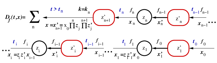
Figure 1: The scheme of integration variables and summation indices in eq. (10); the circles correspond to ${\bf K}^{A}(t_{i})$ and the ovals to ${\bf G}_{{\bf K}^{B}}$, $z_{i}^{\prime}=x_{i}^{\prime}/x_{i-1}$ and $z_{i}=x_{i}/x_{i}^{\prime}$.

In the following we are going to nest eq. (8) twice. First, we employ it in order to isolate gluonstrahlung and flavour-changing parts of the evolution, exploiting the following split of the kernel

$$\mathcal{K}(t)_{ff^{\prime}}=\mathcal{K}^{A}(t)_{ff^{\prime}}+\mathcal{K}^{B}(t)_{ff^{\prime}}=(1-\delta_{ff^{\prime}})\mathcal{K}(t)_{ff^{\prime}}+\delta_{ff^{\prime}}\mathcal{K}(t)_{ff}.$$ (9)

In this case ${\bf G}_{{\bf K}^{B}}$ represents pure gluonstrahlung and is diagonal in the flavour index. In the standard integro-tensorial notation eq. (8) looks as follows:

$$\begin{split}D_{f}(t,x)=&\int\limits_{x}^{1}dx_{0}\;G_{ff}(K^{B};t,t_{0};x,x_{0})\;D_{f}(t_{0},x_{0})+\sum_{n=1}^{\infty}\;\sum_{f_{n-1},\dots,f_{1},f_{0}}\\ \times&\int\limits_{x}^{1}dx_{0}\;\Bigg{[}\prod_{i=1}^{n}\int\limits_{t_{i-1}}^{t}dt_{i}\;\int\limits_{0}^{1}dx_{i}\;\int\limits_{0}^{1}dx^{\prime}_{i}\;\theta_{x_{i}<x^{\prime}_{i}<x_{i-1}}\Bigg{]}\;G_{ff}(K^{B};t,t_{n},x,x_{n})\;\\ \times&\Bigg{[}\prod_{i=1}^{n}\mathcal{K}^{A}_{f_{i}f_{i-1}}(t_{i},x_{i},x^{\prime}_{i})\;G_{f_{i-1}f_{i-1}}(K^{B};t_{i},t_{i-1},x^{\prime}_{i},x_{i-1})\Bigg{]}\;D_{f_{0}}(t_{0},x_{0}),\end{split}$$ (10)

where $f_{n}\equiv f$. In the above and the following equations we adopt the following notation:

$$\delta_{x=y}=\delta(x-y)$$

and

$$\theta_{y<x}=1~{}~{}~{}\hbox{\rm for}~{}~{}~{}y<x~{}~{}~{}\hbox{\rm and}~{}~{}~{}\theta_{y<x}=0~{}~{}~{}\hbox{\rm for}~{}~{}~{}y\geq x.$$

Similarly, $\theta_{z<y<x}=\theta_{z<y}\theta_{y<x}$. The chain of integration variables and flavour indices is depicted schematically in Fig. 1.

Next, eq. (8) is used in order to resum the virtual IR-divergent part $\mathcal{K}^{V}$ of the gluonstrahlung kernel $\mathcal{K}^{B}$

$$\begin{split}&\mathcal{K}^{B}_{ff^{\prime}}(t,x,u)=\delta_{ff^{\prime}}\mathcal{K}_{ff}(t,x,u)=\delta_{ff^{\prime}}\;\big{(}\mathcal{K}^{V}_{ff}(t,x,u)+\mathcal{K}^{R}_{ff}(t,x,u)\big{)},\\ &\mathcal{K}^{V}_{ff}(t,x,u)=-\delta_{x=u}\mathcal{K}^{v}_{ff}(t,x),\\ &\mathcal{K}^{R}_{ff}(t,x,u)=\theta_{x<u-\Delta(x,u)}\mathcal{K}_{ff}(t,x,u),\end{split}$$ (11)

where $\Delta(x,u)$ is finite IR cut-off, not necessarily infinitesimal. In order to resum (exponentiate) the virtual part $\mathcal{K}^{V}$ of the kernel the following version of eq. (8) is employed

$$\begin{split}&{\bf G}_{{\bf K}^{V}+{\bf K}^{R}}(t,t_{0})={\bf G}_{{\bf K}^{V}}(t,t_{0})\;+\\ &~{}~{}~{}~{}~{}~{}~{}~{}~{}~{}~{}~{}~{}+\sum_{n=1}^{\infty}\left[\prod_{i=1}^{n}\int_{t_{0}}^{t}dt_{i}\;\theta_{t_{i}>t_{i-1}}{\bf G}_{{\bf K}^{V}}(t_{i+1},t_{i}){\bf K}^{R}(t_{i})\right]{\bf G}_{{\bf K}^{V}}(t_{1},t_{0}).\end{split}$$ (12)

Since ${\bf K}^{V}(t_{i})$ is diagonal in $x$, $u$ and in the flavour index, and also because of

$$\{G_{{\bf K}^{V}}(t_{i+1},t_{i})\}_{ff}(x,u)=\delta_{x=u}\;e^{-\Phi_{f}(t_{i+1},t_{i}|x)},\qquad\Phi_{f}(t_{i+1},t_{i}|x)=\int_{t_{i}}^{t_{i+1}}dt\;\mathcal{K}^{v}_{ff}(t,x),$$ (13)

we obtain immediately

$$\begin{split}G_{ff}(K^{B};t_{b},t_{a},x,u)\equiv\{&{\bf G}_{{\bf K}^{B}}(t_{b},t_{a})\}_{ff}(x,u)=\\ =e^{-\Phi_{f}(t_{b},t_{a}|x)}\delta_{x=u}+&\sum_{n=1}^{\infty}\;\bigg{[}\prod_{i=1}^{n}\int_{t_{a}}^{t_{b}}dt_{i}\;\theta_{t_{i}>t_{i-1}}\int_{x}^{u}dx_{i}\theta_{x_{i}<x_{i-1}}\bigg{]}\\ &\times e^{-\Phi_{f}(t_{b},t_{n}|x)}\bigg{[}\prod_{i=1}^{n}\mathcal{K}^{R}_{ff}(t_{i},x_{i},x_{i-1})e^{-\Phi_{f}(t_{i},t_{i-1}|x_{i-1})}\bigg{]}\delta_{x=x_{n}},\end{split}$$ (14)

where $t_{n+1}\equiv t_{b}$, $t_{0}\equiv t_{a}$ and $x_{0}\equiv u$. The above result can also be obtained by iterating the evolution equation for ${\bf G}_{{\bf K}^{B}}(t,t_{0})$ with the boundary condition ${\bf G}_{{\bf K}^{B}}(t_{0},t_{0})={\bf I}$, see for instance ref. [17].

The algebra resulting from (8) is quite general and does not rely on any particular form of the kernel. For example, in the above calculations we did not have to invoke the energy sum rules, or any other specific restrictions on the overall normalization embodied usually in the virtual corrections. Also, we did not define yet the relation between the evolution variables $t_{i}$ and $x_{i}$ and parton four-momenta. This will be done in the following section.

3 Evolution kernel and variables

Before we specify details of the evolution kernels used in this work, let us discuss the relation between the evolution variables $x_{j}$, $t_{j}$ and the emitted parton four-momenta $k_{j}^{\mu}$ in the corresponding parton shower MC.

In the proofs of the factorization theorems [1, 18, 2] and its practical realizations like in ref. [19], typically within $\overline{MS}$ scheme, one projects the four-momenta of the (off-shell) partons into the 1-dimensional variable of the evolution, typically the dimensionless lightcone variable $x$. The so-called factorization scale $\mu_{F}=Q$ measuring the size of the available parton emission phase space is usually set by the kinematics of the hard process. The underlying QCD differential distribution (the QCD matrix element times the phase space) is reduced to a chain of parton splittings with the $x$ variable of the PDF being the fraction of the initial hadron energy $E_{h}$ carried by the parton entering the hard process. The variable $e^{t}=Q$ defines the boundary (maximum value) for many ordered variables $t_{i}$. The variable $t$ may be related directly to one of the phase space parameters (virtuality, transverse momentum, angle) or the abstract dimensional scale variable $\mu_{F}$ resulting from the formal procedure of cancelling IR singularities in the dimensional regularization method. In the classical construction of the parton shower MC, one must invert the above mapping of the phase space variables into the evolution variables; that is to construct parton four-momenta out of $t_{i}$ and $x_{i}$ and to reconstruct fully differential parton distributions in terms of these four-momenta. Obviously this procedure is not unique and requires some guidance from the detailed knowledge of the structure of the IR singularities of the original QCD matrix element.

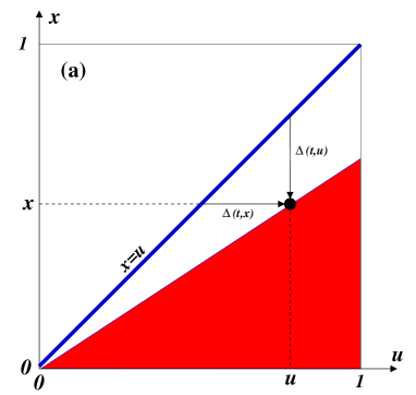
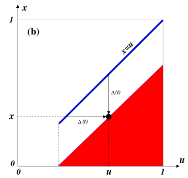
Figure 2: Two types of the infrared (IR) boundaries on the $u-x$ plane (a) $u-x>u\epsilon$ and (d) $u-x>\epsilon$ for the triangle (red) which depicts the area where the real emission part ${\cal K}^{\theta}$ is nonzero. The diagonal line (blue) represents places where the virtual ${\cal K}^{v}$ is nonzero.

In this work we shall construct the CMC algorithm for two new types of generalized kernels, in addition to the ones of LL DGLAP of eq. (2) for which examples of CMC were already constructed in refs. [8] and [9]. The new kernels are based on the following generic form

$$\begin{split}&{\cal K}_{ff^{\prime}}(t,x,u)=\frac{\alpha_{S}(t,x,u)}{\pi}\frac{1}{u}P_{ff^{\prime}}^{(0)}\left(t,\frac{x}{u}\right)=-{\cal K}^{v}_{ff}(t,u)\delta_{ff^{\prime}}\delta_{x=u}+{\cal K}^{\theta}_{ff^{\prime}}(t,x,u),\\ &{\cal K}^{\theta}_{ff^{\prime}}(t,x,u)={\cal K}_{ff^{\prime}}(t,x,u)\theta_{u\geq x+\Delta(t,u)},\end{split}$$ (15)

where $P_{ff^{\prime}}^{(0)}(t,z)$ is the standard LL kernel (DGLAP) and $t$-dependence enters into it only through the IR regulator $\Delta(t,u)$. The new kernel types correspond to different choices of the argument of the strong coupling constant and to different forms of the $\Delta(t,u)$ regulator. The two new types of the regulator $\Delta(t,u)$ used in this work are depicted on the $x-u$ plane in Fig. 2 and will be defined in the following section.

The other important departure from DGLAP is the strong coupling constant $\alpha_{S}(t,x,u)$ which now may depend on all evolution variables. We shall consider the strong coupling constant $\alpha_{S}$ depending on $z=x/u$ or on the transverse momentum $k^{T}$ defined below. Before we define the evolution kernel in a detail, we have to elaborate first the mapping of the evolution variables into four-momenta.

3.1 Relating evolution variables to four-momenta

The essential decision in the construction of the parton shower MC concerns the choice of a kinematics variable in the solutions of the evolution equations (10) and (14); this choice is in one-to-one correspondence with the evolution time variable $t_{i}$ and the limiting value $t$. We choose to associate $t$ with the rapidity (angle) of the emitted parton, following the well known arguments on the colour coherence exposed in many papers, see for instance refs. [20, 21, 22] and further references therein.

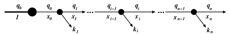
Figure 3: Kinematics in the evolution history (tree).

We define the lightcone variables $q^{\pm}=q^{0}\pm q^{3}$ and normalize the parton momenta with respect to the energy $E_{h}$ of the initial massless hadron, see Fig. 3,

$$q_{h}^{+}=2E_{h},\quad{\rm and}\quad q_{i}^{+}=x_{i}2E_{h},\quad{\rm where}\quad 0\leq x_{i}\leq 1.$$ (16)

These relations hold in the rest frame of the hard process system (HRS) with the $z$-axis along the momentum of initial state hadron $h$.

In particular, for the parton initiating a parton cascade, we have

$$q_{0}^{+}=x_{0}2E_{h}.$$ (17)

This parton has negligible transverse momentum, $k_{0}^{T}=0$. In the HRS each on-shell $i$-th emitted particle will take away a part of the lightcone variable

$$k_{i}^{+}=q_{i-1}^{+}-q_{i}^{+}=(x_{i-1}-x_{i})2E_{h}.$$ (18)

The above is not enough to define $k^{\mu}$. For this we need to define at least $k^{T}=|\vec{k}^{T}|$ or the rapidity $\eta_{i}=\frac{1}{2}\ln(k_{i}^{+}/k^{-}_{i})$. Once the azimuthal angle $\varphi_{i}$ is added, we can complete the mapping from the evolution variables to the 4-momentum of the $i$-th emitted parton $k^{\mu}_{i}(t_{i},x_{i},x_{i-1},\varphi_{i})$.

If we associate the evolution time $t_{i}$ with the rapidity $\eta_{i}$ then the following relation

$$k_{i}^{T}=\sqrt{k_{i}^{+}k^{-}_{i}}=k_{i}^{+}\sqrt{\frac{k^{-}_{i}}{k^{+}_{i}}}=k_{i}^{+}e^{-\eta_{i}}=(x_{i-1}-x_{i})2E_{h}e^{-\eta_{i}},$$ (19)

valid for $k^{2}_{i}=0$, provides the transverse momentum and thus $k_{i}^{\mu}$. We can also eliminate $k_{i}^{T}$ with the help of the following conventional relation which defines the evolution time $t$

$$k_{i}^{T}\equiv e^{t_{i}}(x_{i-1}-x_{i}).$$ (20)

Note that this relation translates into $k^{T}=e^{t}(u-x)$ in the general evolution equation of eq. (1). We observe that evolution time $t_{i}$ and rapidity $\eta_{i}$ are related by a linear transformation of the following explicit form:

$$e^{t_{i}}=e^{\ln(2E_{h})-\eta_{i}}\quad\Rightarrow\quad\eta_{i}=\ln(2E_{h})-t_{i}.$$ (21)

The above relation is the main result of this section.

Summarizing, the mapping of $t_{i}$ and $x_{i}$ into 4-momenta $k^{\mu}_{i},i=1,2,\ldots n$, can be written now in an explicit manner:

$$\begin{split}&k_{i}^{+}=(x_{i-1}-x_{i})2E_{h},\qquad k_{i}^{T}=(x_{i-1}-x_{i})e^{t_{i}},\qquad k_{i}^{-}=(k_{i}^{T})^{2}/k_{i}^{+},\\ &k_{i}^{0}=(k_{i}^{+}+k_{i}^{-})/2,\qquad~{}~{}~{}~{}k_{i}^{3}=(k_{i}^{+}-k_{i}^{-})/2.\end{split}$$ (22)

Last but not least, we have to define also the phase space limits, $t_{i}\in(t_{\min},t_{\max})$ and $\eta_{i}\in(\eta_{\min},\eta_{\max})$. One has to be very careful at this step. The maximum evolution time $t_{\max}$ (minimum rapidity $\eta_{\min}$) is set by the requirement that all emitted partons are confined to the forward hemisphere, $90^{\circ}\geq\theta_{i}$, or equivalently $\eta_{i}\geq\eta_{\min}=0$. This implies

$$t_{\max}=\ln(2E_{h}),\quad E_{h}=\frac{1}{2}e^{t_{\max}}.$$ (23)

The minimum evolution time is determined by the phase space opening point for the first emission, due to minimum transverse momentum $k^{T}_{\min}=\lambda$:

$$e^{t_{1}}x_{0}\geq\lambda.$$ (24)

This leads to

$$t_{1}>t_{{}_{\lambda}}-\ln x_{0},\quad t_{\lambda}\equiv\ln\lambda$$

and therefore to

$$t>t_{n}>t_{n-1}>\ldots>t_{2}>t_{1}>t_{{}_{\lambda}}-\ln x_{0}\equiv t_{\min}.$$

This automatically determines the maximum rapidity

$$\eta_{\max}=\ln(2E_{h})-\ln\lambda+\ln x_{0}.$$

Altogether

$$\begin{split}&t_{i}\in(t_{\min},t_{\max})=(\ln\lambda-\ln x_{0},\ln(2E_{h})),\\ &\eta_{i}\in(\eta_{\min},\eta_{\max})=(0,\ln(2E_{h})+\ln x_{0}-\ln\lambda)),\\ &\eta_{\max}-\eta_{\min}=t_{\max}-t_{\min}=\ln(2E_{h}/\lambda).\end{split}$$ (25)

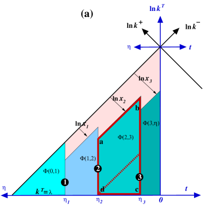
Figure 4: Sudakov plane parametrized using two different sets of variables: (a) $(t,v)$ and/or $(\eta,\ln k^{T})$, (b) $(\bar{t},v)$, where $\bar{t}=t-\ln\Lambda_{0}$, see Appendix. For simplicity $x_{0}=1$ is set. Dashed red line marks position of the Landau pole.

Let us remark that the naive assignment $t_{\max}=\ln(E_{h})$, without the factor of 2, would lead, because of eq. (21), to a partial coverage of the forward hemisphere only, $\eta_{i}\geq\ln(2)$. On the other hand, this factor of 2 may look justified; the absolute kinematic range of the transverse momentum is $k_{i}^{T}\in(\lambda,k_{\max}^{T})$, where $k_{\max}^{T}=e^{t_{\max}}=2E_{h}$ results from the relation $k_{i}^{T}\equiv e^{t_{i}}(x_{i-1}-x_{i})$ and energy conservation $x_{i}\leqslant 1$. The reader may notice that this limit is a factor of 2 higher than in the familiar inequality $k^{T}_{i}\leq E_{h}$ resulting from the 4-momentum conservation operating in both hemispheres simultaneously, i.e. on $k_{i}^{+}$ and $k_{i}^{-}$. However, our limit is valid, including the factor of 2, for a single hemisphere separated from any “activity” on the other side!

Finally, we illustrate the real emission phase space in Fig. 4(a) using the rapidity variable $\eta$ and the log of transverse momentum $k^{T}$. Directions of the lightcone variables $k^{\pm}$ are also indicated. In this figure we indicate, as black numbered points, momenta of three example emitted partons. Available phase space is limited from below by $k^{T}_{\min}=\lambda$, while in the direction $k^{+}$ the boundary is controlled by the total available $q^{+}$, which is diminished by the factor $x_{i-1}$ at $i$-the step (setting for simplicity $x_{0}=1$). The minimum rapidity $\eta=0$ limits the emission phase space from the right hand side. The triangle and trapezoids show integration domains of the consecutive form-factors $\Phi_{f}(t_{i},t_{i-1}|x_{i-1})$ in eq. (14), see also section 3.3 and Appendix A.4.

The above mapping of the evolution variables into four-momenta, with the minimum $k^{T}$ and built-in angular ordering, is identical to the one used in refs. [23, 24, 25], up to the following redefinition of the evolution time: $\hat{t}_{i}=\ln E_{h}-\eta_{i}+\ln x_{i-1}=t_{i}+\ln x_{i-1}$. For the redefined $\hat{t}$ we have

$$\hat{t}+\ln x>\hat{t}_{n}+\ln x_{n}>\hat{t}_{n-1}+\ln x_{n-1}>\ldots>\hat{t}_{2}+\ln x_{2}>\hat{t}_{1}+\ln x_{1}>t_{{}_{\lambda}},$$

and consequently $\hat{q}_{i}>\hat{q}_{i-1}z_{i-1}$, with $z_{i}=x_{i}/x_{i-1}$.

3.2 Evolution kernels

Once the phase-space parametrization is explained, we may define our choices for the evolution kernels, introduced so far only in the generic form in eq. (15). The kernels to be used in the CMC in this work will be of three kinds. The main difference between them is in the choice of the variable used as an argument of the coupling constant $\alpha_{S}$. The appearance of the Landau pole in $\alpha_{S}$ will limit the choice of the IR cut-off in the multigluon phase space. Let us define first the gluonstrahlung kernel $f=f^{\prime}$, where $f$ is flavour type, $f=G,q,\bar{q}$, in all three cases. The strong coupling constant will be always taken in the LL approximation

$$\alpha_{S}^{(0)}(q)=\frac{2\pi}{\beta_{0}}\;\frac{1}{\ln q-\ln\Lambda_{0}}.$$ (26)

Case (A): The standard DGLAP LL of ref. [8], which is used here as a reference case:

$$\begin{split}{\cal K}^{\theta(A)}_{ff}(t,x,u)&=\frac{\alpha_{S}(e^{t})}{\pi}\frac{1}{u}P_{ff}^{(0)}(z)\;\theta_{1-z\geq\epsilon}=\frac{\alpha_{S}(e^{t})}{\pi}\frac{1}{u}P_{ff}^{(0)}(x/u)\;\theta_{u-x\geq u\epsilon},\end{split}$$ (27)

where $\epsilon$ is infinitesimally small and $z=x/u$.

Case (B): The argument in $\alpha_{S}$ is $(1-z)e^{t}=k^{T}/u$; such a choice was already advocated in the early work of ref. [26]. For the IR cut-off we use $\Delta(t,u)=\lambda ue^{-t}$, where $\lambda>\Lambda_{0}$. It cannot be infinitesimally small, however, it becomes very small at large $t$. Using $z=x/u$ we define

$$\begin{split}{\cal K}^{\theta(B)}_{ff}(t,x,u)&=\frac{\alpha_{S}^{(0)}((1-z)e^{t})}{\pi}\frac{1}{u}P_{ff}^{(0)}(z)\;\theta_{1-z\geq\lambda e^{-t}}\\ &=\frac{\alpha_{S}^{(0)}((1-x/u)e^{t})}{\pi}\frac{1}{u}P_{ff}^{(0)}(x/u)\;\theta_{u-x\geq u\lambda e^{-t}}\;.\end{split}$$ (28)

Case (C): The coupling constant $\alpha_{S}$ depends on the transverse momentum $k^{T}=(u-x)e^{t}$, while for an IR cut-off we choose $\Delta(t,u)=\Delta(t)=\lambda e^{-t}$. The kernel reads:

$$\begin{split}{\cal K}^{\theta(C)}_{ff}(t,x,u)&=\frac{\alpha_{S}^{(0)}((u-x)e^{t})}{\pi}\frac{1}{u}P_{ff}^{(0)}(x/u)\theta_{u-x\geq\lambda e^{-t}}.\end{split}$$ (29)

For the (B) and (C) cases the choice of $\lambda$ for the IR cut-off must be such that we avoid the Landau pole in – the insertion of the $1-z$ factor to the argument of the coupling constant resums higher order effects in the bremsstrahlung parts of the evolution [26]. In the non-diagonal, flavour-changing, elements of the kernel, there is no need for this kind of resummation. We can, therefore, use $\alpha_{S}(e^{t})$. On the other hand, although quark gluon transition kernel elements have neither IR divergence nor a Landau pole, it makes sense to keep the restriction $u-x<\Delta(t,u)$, because the cut-out part of the phase space is (will be) already populated by the $k^{T}$ distribution of the primordial parton.

3.3 Virtual part of the kernel and form-factors

For the evolution with any type of kernel the momentum sum rule

$$\begin{split}&0=\partial_{t}\sum_{f}\int dx\;xD_{f}(t,x)=\sum_{f}\int^{1}_{0}du\left\{\sum_{f^{\prime}}\int^{u}_{0}dx\;x{\cal K}_{ff^{\prime}}(t,x,u)\right\}D_{f^{\prime}}(t,u)\\ &=\sum_{f}\int^{1}_{0}du\left\{-u{\cal K}^{v}_{ff}(t,u)+\sum_{f^{\prime}}\int_{0}^{u}dx\;x{\cal K}^{\theta}_{ff^{\prime}}(t,x,u)\right\}D_{f^{\prime}}(t,u)\end{split}$$ (30)

is imposed, the same as in the reference DGLAP case.

This sum rule determines unambiguously the virtual part of the kernel for all cases (A–C)

$${\cal K}^{v}_{ff}(t,u)=\sum_{f^{\prime}}\int^{u}_{0}\frac{dx}{u}x\;{\cal K}^{\theta}_{f^{\prime}f}(t,x,u).$$ (31)

It should be stressed, that in case (C) ${\cal K}^{v}(t,u)$ includes implicitly $\theta_{u>\Delta(t)}$, as visualized in Fig. 2(b). The following Sudakov form-factor results immediately:

$$\begin{split}&\Phi_{f}(t_{1},t_{0}|u)=\int^{t_{1}}_{t_{0}}dt\;{{\cal K}^{v}_{ff}(t,u)}=\sum_{f^{\prime}}\int^{t_{1}}_{t_{0}}dt\int_{0}^{u}\frac{dx}{u}x\;{\cal K}^{\theta}_{f^{\prime}f}(t,x,u)\\ &=\sum_{f^{\prime}}\int^{t_{1}}_{t_{0}}dt\int_{0}^{u}\frac{dy}{u}(u-y)\;{\cal K}^{\theta}_{f^{\prime}f}(t,u-y,u)=\sum_{f^{\prime}}\int^{t_{1}}_{t_{0}}dt\int_{0}^{1}dz\;uz{\cal K}^{\theta}_{f^{\prime}f}(t,uz,u),\end{split}$$ (32)

where $z\equiv x/u$ and $y\equiv u-x=(1-z)u$. The ${\cal K}^{\theta}_{f^{\prime}f}$ is constructed using the IR-singular, non-singular and flavour-changing parts of the DGLAP (LL) kernel according to the following decomposition

$$zP_{f^{\prime}f}^{\theta}(z)=\biggl{[}\delta_{f^{\prime}f}\left(\frac{A_{ff}}{1-z}+F_{ff}(z)\right)+(1-\delta_{f^{\prime}f})F_{f^{\prime}f}(z)\biggr{]}\theta_{u-x>\Delta(u)}.$$ (33)

For the list of the coefficients $A_{ff}$ and the functions $F_{f^{\prime}f}(z)$ see Appendix of ref. [17].

We also need to define the generalized kernels beyond the case of bremsstrahlung, that is for the quark gluon transitions. One of the possible extensions, valid for all three cases $X=A,B,C$, reads

$$x{\cal K}^{\theta(X)}_{f^{\prime}f}(t,x,u)=\delta_{f^{\prime}f}\;x{\cal K}^{\theta(X)}_{f^{\prime}f}(t,x,u)+(1-\delta_{f^{\prime}f})\frac{\alpha_{S}(e^{t})}{\pi}F_{f^{\prime}f}(z)\theta_{u-x>\Delta^{(X)}(u)},$$ (34)

where $\alpha_{S}$ in the flavour changing elements has no $z$- or $k^{T}$-dependence and the IR cut-off $\Delta^{(X)}$ is the same as in the bremsstrahlung case. The Sudakov form-factors resulting from the above kernels are split into three corresponding parts:

$$\Phi_{f}(t_{1},t_{0}|u)=\mathbf{\Phi}_{f}(t_{1},t_{0}|u)+\Phi^{b}_{f}(t_{1},t_{0}|u)+\Phi^{c}_{f}(t_{1},t_{0}|u).$$ (35)

In case (C) we get three genuinely $u$-dependent components

$$\begin{split}\mathbf{\Phi}_{f}(t_{1},t_{0}|u)&=\int^{t_{1}}_{t_{0}}dt\;\int_{0}^{1}dz\;\frac{\alpha_{S}((1-z)ue^{t})}{\pi}\frac{A_{ff}}{1-z}\theta_{(1-z)u>\lambda e^{-t}}\\ &=A_{ff}\frac{2}{\beta_{0}}\varrho_{2}({\bar{t}}_{0}+\ln u,{\bar{t}}_{1}+\ln u;{\bar{t}}_{\lambda}),\\ \Phi^{b}_{f}(t_{1},t_{0}|u)&=\int^{t_{1}}_{t_{0}}dt\;\int_{0}^{1}dz\;\frac{\alpha_{S}((1-z)ue^{t})}{\pi}F_{ff}(z)\;\theta_{(1-z)u>\lambda e^{-t}}\;,\\ \Phi^{c}_{f}(t_{1},t_{0}|u)&=\int^{t_{1}}_{t_{0}}dt\;\frac{\alpha_{S}(e^{t})}{\pi}\sum_{f^{\prime}\neq f}\int_{0}^{1}dz\;F_{f^{\prime}f}(z)\;\theta_{(1-z)u>\lambda e^{-t}},\end{split}$$ (36)

where ${\bar{t}}_{i}\equiv t_{i}-\ln\Lambda_{0}$, ${\bar{t}}_{\lambda}\equiv t_{\lambda}-\ln\Lambda_{0}$ and function $\varrho_{2}$ is defined in Appendix A.2 in terms of log functions. The integration domains for the consecutive form-factors of the above type are also shown in a pictorially way in Fig. 4, using the well known logarithmic Sudakov plane.

In case (B) the $u$ dependence disappears due to the fact that both $\alpha_{S}((1-z)e^{t})$ and $\theta_{1-z>\Delta(t)}$ depend on $u$ exclusively through $z=x/u$:

$$\mathbf{\Phi}_{f}(t_{1},t_{0})=\mathbf{\Phi}_{f}(t_{1},t_{0}|1),\qquad\Phi^{b}_{f}(t_{1},t_{0})=\Phi^{b}_{f}(t_{1},t_{0}|1),\qquad\Phi^{c}_{f}(t_{1},t_{0})=\Phi^{c}_{f}(t_{1},t_{0}|1).$$ (37)

In other words, setting $u=1$ brings us from case (C) to the case (B).

The reason behind the seemingly at hoc three-fold split of $\mathbf{\Phi}_{f}(t_{1},t_{0})$ is practical. In the MC the form-factor has to be calculated event-per-event. One-dimensional integration for each MC event is acceptable – it does not slow down MC generation noticeably. Here, the most singular part of ${\bf\Phi}_{f}$ is calculable analytically. In $\Phi^{b}_{f}$ we are able to integrate analytically over $t$ and the integration over $z$ is done numerically while in $\Phi^{c}_{f}$ we can integrate analytically over $z$ and the integration over $t$ is has to be done numerically (see also Appendix A.3). Altogether, we are thus able to avoid 2-dimensional numerical integration for each MC event (or use of look-up tables and interpolation for fast evaluation of the Sudakov form-factors for each MC event).

Finally, the form-factors for the simplest DGLAP LL case read as follows:

$$\begin{split}\mathbf{\Phi}_{f}(t_{1},t_{0})&=\frac{2}{\beta_{0}}\;(\tau(t_{1})-\tau(t_{0}))\;A_{ff}\ln\frac{1}{\epsilon},\\ \Phi^{b}_{f}(t_{1},t_{0})&=\frac{2}{\beta_{0}}\;(\tau(t_{1})-\tau(t_{0}))\int_{0}^{1}dz\;F_{ff}(z)\;\theta_{1-z>\epsilon}\;,\\ \Phi^{c}_{f}(t_{1},t_{0})&=\frac{2}{\beta_{0}}\;(\tau(t_{1})-\tau(t_{0}))\sum_{f^{\prime}\neq f}\int_{0}^{1}dz\;F_{f^{\prime}f}(z)\;\theta_{1-z>\epsilon}\;,\end{split}$$ (38)

where $\tau(t)=\ln(t-\ln\Lambda_{0})$.

At present, in the MC implementation, we use for cases (B) and (C), a slightly different form of the quark gluon changing kernels elements:

$$\begin{split}&x{\cal K}^{\theta(B^{\prime})}_{f^{\prime}f}(t,x,u)=\delta_{f^{\prime}f}\;x{\cal K}^{\theta(B)}_{f^{\prime}f}(t,x,u)+(1-\delta_{f^{\prime}f})\frac{\alpha_{S}((1-z)e^{t})}{\pi}F_{f^{\prime}f}(z)\theta_{1-z>\lambda e^{-t}}\;,\\ &x{\cal K}^{\theta(C^{\prime})}_{f^{\prime}f}(t,x,u)=\delta_{f^{\prime}f}\;x{\cal K}^{\theta(C)}_{f^{\prime}f}(t,x,u)+(1-\delta_{f^{\prime}f})\frac{\alpha_{S}(u(1-z)e^{t})}{\pi}F_{f^{\prime}f}(z)\theta_{y>\lambda e^{-t}}\;,\end{split}$$ (39)

that is, we use the same arguments of $\alpha_{S}$ as for gluonstrahlung. We will refer to them as cases (B’) and (C’). This is done mainly to facilitate numerical comparisons with our Markovian MCs. One can easily go back from cases (B’) and (C’) to (B) and (C) with an extra (well behaving) MC weight, if needed. The corresponding form-factor $\Phi^{c}_{f}(t_{1},t_{0})$ gets properly redefined in cases (B’) and (C’), of course.

4 Constrained Monte Carlo for pure bremsstrahlung

Let us discuss the case of pure gluonstrahlung first. We will focus our attention on the following integral, being part of eq. (14)

$$\begin{split}G^{n}_{ff}(K^{B};t_{b},t_{a},x,u)&=\bigg{[}\prod_{i=1}^{n}\int_{t_{i-1}}^{t_{b}}dt_{i}\;\int_{x}^{u}dx_{i}\;\mathcal{K}^{R}_{ff}(t_{i},x_{i},x_{i-1})\bigg{]}e^{-\sum_{n=1}^{n+1}\Phi_{f_{i-1}}(t_{i},t_{i-1}|x_{i-1})}\delta_{x=x_{n}}.\end{split}$$ (40)

It describes the emission of $n$ gluons. The following “aliasing” of variables is used: $t_{n+1}\equiv t_{b}$, $t_{0}\equiv t_{a}$ and $x_{0}\equiv u$. The integrand is well approximated by the product of the IR singularities in terms of variables $y_{i}=x_{i}-x_{i-1}$

$$\prod_{i=1}^{n}\mathcal{K}^{R}_{ff}(x_{i},x_{i-1})\simeq\prod_{i=1}^{n}\frac{1}{x_{i}-x_{i-1}}=\prod_{i=1}^{n}\frac{1}{y_{i}}\simeq\prod_{i=1}^{n}\frac{1}{1-z_{i}}.$$ (41)

Hence, switching from variables $x_{i}$ to $y_{i}$ or $z_{i}$ is almost mandatory and the multigluon distribution with the $\delta$-function constraining the total energy of emitted gluons takes the following symmetric form:

$$\int\delta_{x=x_{n}}\prod_{i=1}^{n}\frac{dx_{i}}{x_{i}-x_{i-1}}=\int\delta\left(u-x-\sum_{j=1}^{n}y_{j}\right)\prod_{i=1}^{n}\frac{dy_{i}}{y_{i}}\simeq\int\delta\left(x-u\prod_{j=1}^{n}z_{j}\right)\prod_{i=1}^{n}\frac{dz_{i}}{1-z_{i}}.$$ (42)

Constructing the MC program/algorithm for the multidimensional distribution featuring such a $\delta$-function is a hard technical problem and it is the problem of constructing a Constrained Monte Carlo (CMC).

It should be kept in mind, that it is possible, as shown in ref. [9], to generate the above distribution in $x$-space without such a $\delta$-function, provided $G_{ff}$ is convoluted with the power-like function $x_{0}^{\omega}$. Such a solution was labeled as CMC class II, while the CMC of this paper was already referred to in ref. [9] as CMC class I.

In ref. [8] the first CMC algorithm of the class I was found and tested for DGLAP kernel, that is for our case (A). This algorithm is based on the observation that for the product of steeply rising functions, proportional to $1/y_{i}$, the $\delta$-function constraint is effectively resolved by a single (let’s say) $y_{k}$, while all other $y_{i}$, can be considered as unconstrained. We shall extend the CMC class I solution to more complicated kernels, that is of our type (B) and (C). The main complication with respect to case (A) is due to a more complicated singular $y$-dependence (or $z$-dependence) entering through the coupling constant $\alpha_{S}$, and even more important, through form-factors. In addition, our new CMCs will not only generalize the solutions of ref. [8], but will be described in such a way that any future extension to other types of evolution kernels will be rather easy. In the following sub-sections we shall present the details of our generalized solutions.

4.1 Generic CMC class I

As already indicated, we intend to introduce the formulation of the CMC algorithm which covers three types of kernels (A–C), and also that further extensions are possible and easy. At first, let us consider the following generic expression including the sum of constrained multidimensional integrals

$$D(v)=\Psi^{\prime}(v)\;e^{-\int_{v_{0}}^{v_{x}}K(v^{\prime})dv^{\prime}}\bigg{\{}\delta_{\Psi(v)=\Psi(v_{0})}+\sum_{n=1}^{\infty}\frac{1}{n!}\bigg{[}\int_{v_{0}}^{v}\prod_{i=1}^{n}K(v_{i})dv_{i}\bigg{]}\delta_{\Psi(v)=\sum_{j=1}^{n}\Psi(v_{j})}\bigg{\}}.$$ (43)

The following properties will be assumed: (a) The function $\Psi(v)$, used to change integration variables, must be monotonous; its derivative must remain non-negative, $\frac{d\Psi}{dv}=\Psi^{\prime}(v)\geq 0$, for all $v>v_{0}$. (b) The positioning of the IR term $\delta(v-v_{0})$ at $v=v_{0}$ is a convention. In practical MC realization it represents a no-emission event. Let us stress that in the $v$-space we are free to place the position $v_{IR}$ of the IR part of spectrum $\delta(v-v_{IR})$ anywhere outside the $(v_{0},v_{x})$ interval; we have opted for $v_{IR}=v_{0}$ (c) the variable $v_{x}$ controlling the overall normalization will be specified only later; it will be adjusted to get convenient normalization, (d) the true upper integration limit of $v_{i}$ is below $v$ and is in fact uniquely determined by the $\delta$-function of the constraint.

In the following examples, the variable $v_{i}$ will be defined as $v_{i}=\ln y_{i}=\ln x_{i}-x_{i-1}$ or $v_{i}=\ln(1-z_{i})=\ln(1-x_{i}/x_{i-1})$, while the function $\Psi(v)$ will be typically rather simple; $\Psi(y_{i})=y_{i}$ or $\Psi(z_{i})=\ln z_{i}$.

Assuming $K(v)>0$, we can define a mapping (and its inverse) which removes $K(v)$ from the integrand:

$$r_{i}=R(v_{i})=\int_{v_{0}}^{v_{i}}K(v^{\prime})dv^{\prime},\qquad v_{i}=V(r_{i})=R^{-1}(r_{i}).$$ (44)

Our master formula transforms then as follows:

$$D(v)=\Psi^{\prime}(v)e^{-R(v_{x})}\bigg{\{}\delta_{\Psi(v)=\Psi(v_{0})}+\sum_{n=1}^{\infty}\frac{1}{n!}\bigg{[}\int_{0}^{R(v)}\prod_{i=1}^{n}dr_{i}\bigg{]}\delta_{\Psi(v)=\sum_{j=1}^{n}\Psi(R^{-1}(r_{j}))}\bigg{\}}.$$ (45)

The function $f(r)=\Psi(R^{-1}(r))$ is usually a very steeply growing function of $r$, hence the constraint is effectively resolved by a single $r_{j}\simeq R(v)$, the biggest one. Let us exploit this fact in order to replace the complicated constraint with the simpler one $\delta(R(v)-\max_{j}r_{j})$. This is done in three steps. Step one: introduce a new auxiliary integration variable $X$ countered by a $\delta$-function:

$$\begin{split}D(v)=&e^{-R(v_{x})}\delta_{v=v_{0}}+\Psi^{\prime}(v)e^{-R(v_{x})}\\ &\times\sum_{n=1}^{\infty}\frac{1}{n!}\int dX\bigg{[}\int_{0}^{R(v)}\prod_{i=1}^{n}dr_{i}\bigg{]}\delta_{\Psi(v)=\sum_{j=1}^{n}\Psi(R^{-1}(r_{j}))}\delta_{R(v)=X+\max_{j}r_{j}}.\end{split}$$ (46)

Step two: change the variables $r_{i}=r^{\prime}_{i}-X$:

$$\begin{split}D(v)=&e^{-R(v_{x})}\delta_{v=v_{0}}+\Psi^{\prime}(v)e^{-R(v_{x})}\\ &\times\sum_{n=1}^{\infty}\frac{1}{n!}\int dX\bigg{[}\int_{0}^{R(v)}\prod_{i=1}^{n}dr^{\prime}_{i}\;\theta_{r_{i}>0}\bigg{]}\delta_{\Psi(v)=\sum_{j=1}^{n}\Psi(R^{-1}(r^{\prime}_{j}-X))}\delta_{R(v)=\max_{j}r^{\prime}_{j}}.\end{split}$$ (47)

From now on we have to watch out for the condition $r_{i}=r^{\prime}_{i}-X>0$ explicitly. Step three: eliminate the old constraint by integrating over $X$

$$D(v)=e^{-R(v_{x})}\delta_{v=v_{0}}+e^{-R(v_{x})}\sum_{n=1}^{\infty}\frac{1}{n!}\bigg{[}\int_{0}^{R(v)}\prod_{i=1}^{n}dr^{\prime}_{i}\;\theta_{r_{i}>0}\bigg{]}\delta_{R(v)=\max_{j}r^{\prime}_{j}}\;\mathfrak{J},$$ (48)

where $X_{0}(r^{\prime}_{1},r^{\prime}_{2},...,r^{\prime}_{n})$ is found by means of solving numerically (iterative method) the original constraint for $X$. The Jacobian factor $\mathfrak{J}$ is defined as follows

$$\mathfrak{J}=\frac{\Psi^{\prime}(v)}{\partial_{X}\sum_{j=1}^{n}\Psi(R^{-1}(r^{\prime}_{j}-X_{0}))}=\frac{\Psi^{\prime}(v)}{\sum_{j=1}^{n}\Psi^{\prime}(v_{j})(R^{\prime}(v_{j}))^{-1}}.$$ (49)

In the above factor the $j$-th term satisfying $R(v)=\max_{j}r^{\prime}_{j}$ dominates the sum in the denominator; consequently $\mathfrak{J}\simeq R^{\prime}(v)=K(v)$. This form, valid in the limit only, we keep explicitly in the integrand, while the remaining part of $\mathfrak{J}$ is incorporated in a complicated but mild Monte Carlo weight:

$$D(v)=e^{-R(v_{x})}\delta_{v=v_{0}}+R^{\prime}(v)e^{-R(v_{x})}\sum_{n=1}^{\infty}\frac{1}{n!}\bigg{[}\int_{0}^{R(v)}\prod_{i=1}^{n}dr^{\prime}_{i}\bigg{]}\delta_{\max_{j}r^{\prime}_{j}=R(v)}\;w^{\#},$$ (50)

where the MC weight is

$$w^{\#}=\frac{\Psi^{\prime}(v)}{R^{\prime}(v)\sum_{j=1}^{n}\Psi^{\prime}(v_{j})(R^{\prime}(v_{j}))^{-1}}\prod_{i=1}^{n}\theta_{r_{i}>0}.$$ (51)

Last but not least, we isolate cleanly a part of the integrand normalized properly to 1 with the help of the integration variable $\xi_{i}=r_{i}/R(v)$ and the Poisson distribution $P(n|\lambda)=\exp(-\lambda)\lambda^{n}/n!$:

$$D(v)=e^{-R(v_{x})}\delta_{v=v_{0}}+R^{\prime}(v)e^{R(v)-R(v_{x})}\sum_{n=1}^{\infty}P(n-1|R(v))\bigg{[}\prod_{i=1}^{n}\int_{0}^{1}d\xi_{i}\bigg{]}\frac{\delta_{\max_{j}\xi_{j}}=1}{n}\;w^{\#}(\xi),$$ (52)

The nice thing is that $\bar{D}(v)$, obtained by neglecting $w^{\#}$, is known analytically

$$\bar{D}(v)=D(v)|_{w^{\#}=1}=e^{-R(v_{x})}\delta_{v=v_{0}}+\theta_{v>v_{0}}R^{\prime}(v)e^{R(v)-R(v_{x})}$$ (53)

and is normalized to 1:

$$\int_{v_{0}}^{v_{x}}\bar{D}(v)dv=e^{-R(v_{x})}+\int_{\exp(-R(v_{x}))}^{1}d\Big{(}e^{R(v)-R(v_{x})}\Big{)}=e^{-R(v_{x})}+\Big{(}1-e^{-R(v_{x})}\Big{)}=1.$$ (54)

The above convenient unitary normalization is achieved by means of identifying $v_{x}$ with the upper limit of $v$, see also below for particular realizations. In the implementation of quark gluon transitions using FOAM [27] (see section 5) one introduces the integration variable $U=U(v)=e^{R(v)-R(v_{x})}\in(0,1)$ and the above equation transforms into

$$\int_{0}^{\exp(-R(v_{x}))}dU+\int_{\exp(-R(v_{x}))}^{1}dU=\int_{0}^{1}dU.$$ (55)

The MC procedure of generating the variables $v$, $n$ and $(v_{1},v_{2},...,v_{n})$ obeying the constraint is the following:

• Generate $v$ according to $\bar{D}(v)$ times whatever the other function of $v$ in the Monte Carlo problem, for that purpose use the variable $U=e^{R(v)-R(v_{x})}\in(0,1)$.

• If $U\leq e^{-R(v_{x})}$ then set $v=v_{0}$ and $n=0$ (no-emission event).

• Otherwise $U$ is translated into $v$ ($v>v_{0}$) and $n>0$ is generated according to $P(n-1|R(v))$.

• Generate the variables $\xi_{i}\in(0,1),i=1,2,...,n$, except one of them: $\xi_{j}=1$, where $j=1,2,...n$ is chosen randomly with the uniform probability.

• The variables $\xi_{i}$ are now translated into $r^{\prime}_{i}$ and the transcendental equation defining the shift $X_{0}$ is solved numerically.

• Once $X_{0}$ is known, then all $v_{i}(r_{i}(r^{\prime}_{i}((\xi_{i})))$ are calculated.

• The MC weight $w^{\#}$ is evaluated; the check on $r_{i}>0$ can be done earlier.

The above algorithm generates weighted MC events $(n;v_{1},v_{2},...,v_{n})$ exactly according to the resumed series of the integrands defining $D(v)$.

4.2 Treatment of $t$-ordering – generic case

In case (A) of the DGLAP kernel, discussed in ref. [8], the $t$-ordering in the integrals of eq. (40) can be easily traded for a $1/n!$ factor, while $K(v)$ in the previous section includes un-ordered integrals $\int dt_{i}$ over the entire available range for each $t_{i}$. However, even in this simple case one has to be careful if one aims not only at the numerical evaluation of the PDF, but also at the proper simulation of the entire MC events $\{n,(t_{1},x_{1}),(t_{2},x_{2}),...,(t_{n},x_{n})\}$. The CMC class I algorithm of ref. [8] (DGLAP) is formulated in terms of $z_{i}=x_{i}/x_{i-1}$; the point is that at the end of the MC algorithm one has to calculate $x_{i}$ using a well defined ordering of $z_{i}$, which is exactly the same as in the sequence of the (originally) un-ordered $t_{i}$. In practice, in the end of the MC generation, one has to order $t_{i}$ and $z_{i}$ simultaneously before calculating $x_{i}=x_{0}z_{1}z_{2}...z_{i}$. This is because the original integrand is symmetric with respect to interchange of the pairs of variables $(t_{i},z_{i})\leftrightarrow(t_{k},z_{k})$ and not with respect to interchanging $t_{i}\leftrightarrow t_{k}$ or $z_{i}\leftrightarrow z_{k}$ done independently. This property we will call the pairwise permutation symmetry.

In our most general case (C), the integrand is not pairwise symmetric, mainly due to nontrivial $x_{i}$-dependency in the form-factor, see eq. (40). In this case, the strategy is such that we introduce a simplified integrand, with the simplified form-factor and simplified kernel $\bar{\mathbbm{P}}$ (the IR-singular part of the kernel), such that the simplified integrand does feature the pairwise permutation symmetry. The above simplifications are immediately and exactly compensated by means of the MC weight $w^{\mathbbm{P}}$, which absorbs all possible pairwise non-symmetry.

Let us translate what has been said above into rigorous algebra. We start from a more sophisticated variant of our generic multi-integral (43), covering all cases (A–C) and possibly other similar cases, but this time including explicitly ordered $t$-integrations:

$$\begin{split}D(t,t_{0}|v)=&\Psi^{\prime}(v)e^{-\int_{t_{0}}^{t}dt^{\prime}\int_{v_{0}(t^{\prime})}^{v_{x}}\bar{\mathbbm{P}}(v^{\prime},t^{\prime})dv^{\prime}}\bigg{\{}\delta_{\Psi(v)=\Psi(v_{0})}+\\ &+\sum_{n=1}^{\infty}\bigg{[}\prod_{i=1}^{n}\int_{t_{i-1}}^{t}dt_{i}\;\int_{v_{0}(t_{i})}^{v}dv_{i}\;\bar{\mathbbm{P}}(t_{i},v_{i})\bigg{]}w^{\mathbbm{P}}({\bf t},{\bf v})\;\delta_{\Psi(v)=\sum_{j=1}^{n}\Psi(v_{j})}\bigg{\}},\end{split}$$ (56)

where $t_{n}\equiv t$. The bold-face variable ${\bf t}$ denotes the entire vector $(t_{1},t_{2},...,t_{n})$ and similar convention is used for the definition of the vector ${\bf v}$.

In order to get rid of the $t$-ordering in the basic MC algorithm we proceed carefully step by step as follows:

1. We introduce formally pairwise symmetrization, i.e. we sum up over all permutations $\mathfrak{P}$ of the pairs of the variables $(v_{i},t_{i})$, compensating by means of the $1/n!$ factor:

   $$\frac{1}{n!}\sum_{\mathfrak{P}}\bigg{[}\prod_{i=1}^{n}\int_{t_{0}}^{t}dt^{\mathfrak{P}}_{i}\;\int_{v_{0}(t^{\mathfrak{P}}_{i})}^{v}dv^{\mathfrak{P}}_{i}\;\bar{\mathbbm{P}}(t^{\mathfrak{P}}_{i},v^{\mathfrak{P}}_{i})\bigg{]}\theta_{t^{\mathfrak{P}}_{n}>t^{\mathfrak{P}}_{n-1}>...>t^{\mathfrak{P}}_{1}}\;w^{\mathbbm{P}}({\bf t}^{\mathfrak{P}},{\bf v}^{\mathfrak{P}}).$$

2. The part of the integrand in the brackets is now perfectly pairwise symmetric and the permutation $\mathfrak{P}$ can be undone in this part:

   $$\frac{1}{n!}\bigg{[}\prod_{i=1}^{n}\int_{t_{0}}^{t}dt_{i}\;\int_{v_{0}(t_{i})}^{v}dv_{i}\;\bar{\mathbbm{P}}(t_{i},v_{i})\bigg{]}\sum_{\mathfrak{P}}\theta_{t^{\mathfrak{P}}_{n}>t^{\mathfrak{P}}_{n-1}>...>t^{\mathfrak{P}}_{1}}\;w^{\mathbbm{P}}({\bf t}^{\mathfrak{P}},{\bf v}^{\mathfrak{P}}).$$

3. The sum over permutations $\sum_{\mathfrak{P}}$ can be dropped out because only one permutation contributes at a given point ${\bf t}=(t_{i},t_{2},...,t_{n})$. This particular permutation we denote by $\mathfrak{P}_{\bf t}$, obtaining:

   $$\begin{split}D(t,t_{0}|&v)=\Psi^{\prime}(v)e^{-\int_{t_{0}}^{t}dt^{\prime}\int_{v_{0}(t^{\prime})}^{v_{x}}\bar{\mathbbm{P}}(v^{\prime},t^{\prime})dv^{\prime}}\bigg{\{}\delta_{\Psi(v)=\Psi(v_{0})}+\\ &+\sum_{n=1}^{\infty}\bigg{[}\prod_{i=1}^{n}\int_{t_{i-1}}^{t}dt_{i}\;\int_{v_{0}(t_{i})}^{v}dv_{i}\;\bar{\mathbbm{P}}(t_{i},v_{i})\bigg{]}\delta_{\Psi(v)=\sum_{j=1}^{n}\Psi(v_{j})}\;w^{\mathbbm{P}}({\bf t}^{\mathfrak{P}_{\bf t}},{\bf v}^{\mathfrak{P}_{\bf t}})\bigg{\}}.\end{split}$$ (57)

4. In the basic MC the weight $w^{\mathbbm{P}}$ is temporarily neglected and $t_{i}$ are generated unordered. The permutation $\mathfrak{P}_{\bf t}$ is then read from the ordering in ${\bf t}=(t_{1},t_{2},...,t_{n})$. It is then used to construct the sequence of $x_{i}$ out of $v_{i}$ and to calculate $w^{\mathbbm{P}}$.

In order to finally bring eq. (57) into the standardized form of eq. (43) we interchange the order of integration over $t_{i}$ and $v_{i}$

$$\int_{t_{i-1}}^{t}dt_{i}\;\int_{v_{0}(t_{i})}^{v}dv_{i}\;\bar{\mathbbm{P}}(t_{i},v_{i})=\int_{v_{0}}^{v}dv_{i}\;\int_{t_{i-1}(v_{i})}^{t(v_{i})}dt_{i}\;\bar{\mathbbm{P}}(t_{i},v_{i})=\int_{v_{0}}^{v}dv_{i}\;K(v_{i})\int_{0}^{1}d\sigma_{i}.$$

The additional change of variables

$$\sigma(t,v)=\frac{\int_{t_{\min}(v)}^{t}dt^{\prime}\;\bar{\mathbbm{P}}(t^{\prime},v)}{\int_{t_{\min}(v)}^{t_{\max}(v)}dt^{\prime}\;\bar{\mathbbm{P}}(t^{\prime},v)}=\frac{\int_{t_{\min}(v)}^{t}dt^{\prime}\;\bar{\mathbbm{P}}(t^{\prime},v)}{K(v)}$$ (58)

allows to map, for every value of $v_{i}$, uniformly distributed $\sigma_{i}$ into $t_{i}$. For a particular realization see Appendix A.3. Luckily, $\sigma_{i}(t_{i})$ can be inverted analytically, i.e. $t_{i}(\sigma_{i},v_{i})$ is available as an analytical formula, for all cases (A–C).

The main purpose of the sub-section, was to obtain the following, ready for the MC implementation, representation of our standardized generic formula:

$$\begin{split}&D(t,t_{0}|v)=\Psi^{\prime}(v)e^{-\int_{v_{0}}^{v_{x}}K(v^{\prime})dv^{\prime}}\bigg{\{}\delta_{\Psi(v)=\Psi(v_{0})}+\\ &~{}~{}~{}~{}~{}~{}~{}~{}~{}~{}~{}~{}~{}+\sum_{n=1}^{\infty}\frac{1}{n!}\bigg{[}\prod_{i=1}^{n}\int_{t_{i-1}}^{t}dt_{i}\;K(v_{i})\int_{0}^{1}d\sigma_{i}\;\bigg{]}\delta_{\Psi(v)=\sum_{j=1}^{n}\Psi(v_{j})}\;w^{\mathbbm{P}}({\bf t}^{\mathfrak{P}_{\bf t}},{\bf v}^{\mathfrak{P}_{\bf t}})\bigg{\}}\\ &~{}~{}=e^{-R(v_{x})}\delta_{v=v_{0}}+\theta_{v>v_{0}}R^{\prime}(v)e^{R(v)-R(v_{x})}\\ &~{}~{}~{}~{}~{}~{}~{}~{}~{}~{}~{}~{}\times\sum_{n=1}^{\infty}P(n-1|R(v))\bigg{[}\prod_{i=1}^{n}\int_{0}^{1}d\xi_{i}\int_{0}^{1}d\sigma_{i}\;\bigg{]}\frac{\delta_{\max_{j}\xi_{j}}=1}{n}\;w^{\#}(\mathbf{\xi})\;w^{\mathbbm{P}}({\bf t}^{\mathfrak{P}_{\bf t}},{\bf v}^{\mathfrak{P}_{\bf t}}).\end{split}$$ (59)

In the following subsection we shall describe three realizations of the above CMC class I schemes for three types of the kernels, (A–C).

4.3 CMC case (A), DGLAP

Let us start with the particular realization of the above CMC for the easiest case of the DGLAP kernel, type (A). Such a CMC was exposed in detail already in ref. [8]. Here it serves as a reference case and a warm-up example. We recall the pure bremsstrahlung evolution operator of eq. (14) in a form adopted for further manipulations:

$$\begin{split}\frac{x}{u}G_{ff}(K^{B};t_{b},t_{a},x,u)&=e^{-\Phi_{f}(t_{b},t_{a})}\delta_{x=u}+\sum_{n=1}^{\infty}\;\bigg{[}\prod_{i=1}^{n}\int_{t_{a}}^{t_{b}}dt_{i}\;\theta_{t_{i}>t_{i-1}}\int_{x}^{u}dx_{i}\bigg{]}\\ &\times e^{-\Phi_{f}(t_{b},t_{n})}\bigg{[}\prod_{i=1}^{n}\frac{x_{i}}{x_{i-1}}\mathcal{K}^{R}_{ff}(t_{i},x_{i},x_{i-1})e^{-\Phi_{f}(t_{i},t_{i-1})}\bigg{]}\delta_{x=x_{n}},\end{split}$$ (60)

where we have dropped the non-existing dependence on $x_{i}$ in the form-factor $\Phi$. Hence, one may exploit the relation $\sum_{i=0}^{n}\Phi(t_{i},t_{i-1})=\Phi(t_{b},t_{a})$. After identification of terms and change of integration variables

$$x_{i}\mathcal{K}^{R}_{ff}(t_{i},x_{i},x_{i-1})=\frac{\alpha_{S}(e^{t_{i}})}{\pi}z_{i}P_{ff}(z_{i})\theta_{1-z_{i}>\epsilon},\qquad z_{i}=x_{i}/x_{i-1},$$

a simplified expression is obtained:

$$\begin{split}&\frac{x}{u}G_{ff}(K^{B};t_{b},t_{a},x,u)=e^{-\Phi_{f}(t_{b},t_{a})}\delta_{x=u}+\\ &~{}~{}~{}~{}~{}~{}+e^{-\Phi_{f}(t_{b},t_{a})}\sum_{n=1}^{\infty}\;\bigg{[}\prod_{i=1}^{n}\int^{t_{b}}_{t_{i-1}}dt_{i}\;\int^{1}_{x/u}dz_{i}\;\frac{\alpha_{S}(e^{t_{i}})}{\pi}z_{i}P_{ff}(z_{i})\theta_{1-z_{i}>\epsilon}\bigg{]}\delta_{x=u\prod_{j=1}^{n}z_{j}}.\end{split}$$ (61)

In the next step, the simplified kernel is introduced

$$\begin{split}&\prod_{i=1}^{n}\int\limits^{1-\epsilon}dz_{i}\;\alpha_{S}(e^{t_{i}})z_{i}P_{ff}(z_{i})\rightarrow\prod_{i=1}^{n}\int\limits^{1-\epsilon}\frac{dz_{i}}{1-z_{i}}\;\alpha_{S}(e^{t_{i}})A_{ff}=\\ &~{}~{}~{}~{}~{}~{}~{}~{}~{}~{}~{}~{}~{}~{}=\prod_{i=1}^{n}\int\limits_{\ln\epsilon}dv_{i}\;\alpha_{S}(e^{t_{i}})A_{ff}=\prod_{i=1}^{n}\int\limits_{v_{0}}dv_{i}\;\bar{\mathbbm{P}}(t_{i},v_{i}),\\ &\bar{\mathbbm{P}}(t_{i},v_{i})=\frac{\alpha_{S}(e^{t_{i}})}{\pi}A_{ff},\quad v_{i}=\ln(1-z_{i}),\quad v_{0}=\ln\epsilon.\end{split}$$ (62)

Once $v$ is defined, we are ready to deduce our kernel $K(v)$ and constraint function $\Psi(v)$ from

$$\begin{split}&\frac{x}{u}G_{ff}(K^{B};t_{b},t_{a},x,u)=e^{-\Phi_{f}(t_{b},t_{a})}\frac{1}{x}\delta_{\ln(x/u)=0}\\ &~{}~{}~{}~{}~{}~{}+e^{-\Phi_{f}(t_{b},t_{a})}\sum_{n=1}^{\infty}\;\bigg{[}\prod_{i=1}^{n}\int\limits^{t_{b}}_{t_{i-1}}dt_{i}\;\int\limits_{v_{0}}^{\ln(1-x/u)}dv_{i}\;\bar{\mathbbm{P}}(t_{i},v_{i})\bigg{]}\frac{1}{x}\delta_{\ln(x/u)=\sum_{j=1}^{n}\ln(1-\exp(v_{j}))}\;w_{1}^{\bar{\mathbbm{P}}},\end{split}$$ (63)

where

$$w_{1}^{\bar{\mathbbm{P}}}=\prod_{i=1}^{n}\frac{\alpha_{S}(e^{t_{i}})z_{i}(1-z_{i})P_{ff}(z_{i})}{\bar{\mathbbm{P}}(t_{i},v_{i})}.$$ (64)

By means of comparison of the above expressions with eq. (56), see also eqs. (44,59), one can identify the components:

$$\begin{split}&v=\ln(1-x/u),\quad\Psi(v)=\ln(1-e^{v}),\quad|\Psi^{\prime}(v)|=\frac{e^{v}}{1-e^{v}}=\frac{u-x}{x},\\ &K(v)=\int_{t_{a}}^{t_{b}}dt\;\bar{\mathbbm{P}}(t_{i},v_{i})=A_{ff}\frac{2}{\beta_{0}}\big{(}\tau(t_{b})-\tau(t_{a})\big{)}.\end{split}$$ (65)

The expression for the basic form-factor can be identified also:

$$R(v)=\int_{v_{0}}^{v}dv^{\prime}\;K(v^{\prime})=\int_{v_{0}}^{v}dv^{\prime}\;\int_{t_{a}}^{t_{b}}dt^{\prime}\;\bar{\mathbbm{P}}(t^{\prime},v^{\prime})=A_{ff}\frac{2}{\beta_{0}}\big{(}\tau(t_{b})-\tau(t_{a})\big{)}(v-v_{0}).$$ (66)

The relation $v=\ln(1-x/u)$ is valid for $v>v_{0}$ only. The variable $v_{x}$ represents the upper boundary of $v=\ln(1-x/u)$, hence or fixed $x$ and maximal $u=1$ we obtain $v_{x}=\ln(1-x)$. With all the above elements at hand, we are able to complete the following standardized, accordingly to conventions of eq. (59), formula

$$\begin{split}&\frac{x}{u}G_{ff}(K^{B};t_{b},t_{a},x,u)=\bigg{\{}e^{-R(v_{x})}\delta_{v=v_{0}}+\theta_{v>v_{0}}\frac{1}{x\Psi^{\prime}(v)}R^{\prime}(v)e^{R(v)-R(v_{x})}\\ &~{}~{}\times\sum_{n=1}^{\infty}P(n-1|R(v))\bigg{[}\prod_{i=1}^{n}\int_{0}^{1}d\xi_{i}\int_{0}^{1}d\sigma_{i}\;\bigg{]}\frac{\delta_{\max_{j}\xi_{j}=1}}{n}\;w^{\#}(\mathbf{\xi})\;w^{\mathbbm{P}}({\bf t}^{\mathfrak{P}_{\bf t}},{\bf v}^{\mathfrak{P}_{\bf t}})\bigg{\}}.\end{split}$$ (67)

where

$$w^{\bar{\mathbbm{P}}}=e^{R(v_{x})-\Phi_{f}(t_{b},t_{a})}\prod_{i=1}^{n}\frac{\alpha_{S}(e^{t_{i}})z_{i}(1-z_{i})P_{ff}(z_{i})}{\bar{\mathbbm{P}}(t_{i},v_{i})}$$ (68)

and the second weight $w^{\#}$ is fully determined from eq. (51), supplemented with $\Psi(v)$ and $K(v)$ of eq. (65).

In the CMC, we usually integrate over $u$ for fixed $x$, hence the following formula is relevant

$$\begin{split}&\int_{x}^{1}duG_{ff}(K^{B};t_{b},t_{a},x,u)=\int_{0}^{1}dU\;\bigg{(}\frac{u}{x}\bigg{)}^{2}\bigg{\{}\theta_{U\leq\exp(-R(v_{x}))}|_{v=v_{0}}+\theta_{U>\exp(-R(v_{x}))}\\ &~{}~{}\times\sum_{n=1}^{\infty}P(n-1|R(v))\bigg{[}\prod_{i=1}^{n}\int_{0}^{1}d\xi_{i}\int_{0}^{1}d\sigma_{i}\;\bigg{]}\frac{\delta_{\max_{j}\xi_{j}=1}}{n}\;w^{\#}(\mathbf{\xi})\;w^{\mathbbm{P}}({\bf t}^{\mathfrak{P}_{\bf t}},{\bf v}^{\mathfrak{P}_{\bf t}})\bigg{\}}.\end{split}$$ (69)

where $U=U(x,u)=e^{R(v)-R(v_{x})}=e^{R(\ln(1-x/u))-R(\ln(1-x))}$. Due to relation $R(v_{0})=0$, the point $v=v_{0}$ (IR boundary) translates into $U_{0}=e^{-R(v_{x})}=e^{-R(\ln(1-x))}$. With all elements needed in eq. (59) at hand, we are ready to reconstruct from our generic formulation the complete CMC class I algorithm of ref. [8], at least for pure bremsstrahlung.

4.4 CMC case (B), $\alpha_{S}(e^{t}(1-z))$

This case is to some extent similar to the previous DGLAP case. We shall, therefore, concentrate on the differences. The starting point is now

$$\begin{split}\frac{x}{u}G_{ff}(K^{B};t_{b},t_{a},x,u)&=e^{-\Phi_{f}(t_{b},t_{a}|1)}\delta_{x=u}+\sum_{n=1}^{\infty}\;\bigg{[}\prod_{i=1}^{n}\int_{t_{a}}^{t_{b}}dt_{i}\;\theta_{t_{i}>t_{i-1}}\int_{x}^{u}dx_{i}\bigg{]}\\ &\times e^{-\Phi_{f}(t_{b},t_{n}|1)}\bigg{[}\prod_{i=1}^{n}\frac{x_{i}}{x_{i-1}}\mathcal{K}^{R}_{ff}(t_{i},x_{i},x_{i-1})e^{-\Phi_{f}(t_{i},t_{i-1}|1)}\bigg{]}\delta_{x=x_{n}},\end{split}$$ (70)

where one may again combine form-factors into a single one: $\sum_{i=0}^{n}\Phi(t_{i},t_{i-1}|1)=\Phi(t_{b},t_{a}|1)$. Now, in terms of

$$x_{i}\mathcal{K}^{R}_{ff}(t_{i},x_{i},x_{i-1})=\frac{\alpha_{S}(e^{t_{i}}(1-z_{i}))}{\pi}z_{i}P_{ff}(z_{i})\theta_{1-z_{i}>\lambda e^{-t_{i}}},\qquad z_{i}=x_{i}/x_{i-1},$$

the simplified expression reads

$$\begin{split}&\frac{x}{u}G_{ff}(K^{B};t_{b},t_{a},x,u)=e^{-\Phi_{f}(t_{b},t_{a}|1)}\bigg{\{}\delta_{x=u}+\\ &~{}~{}+\sum_{n=1}^{\infty}\;\bigg{[}\prod_{i=1}^{n}\int^{t_{b}}_{t_{i-1}}dt_{i}\;\int^{1}_{x/u}dz_{i}\;\frac{\alpha_{S}((1-z_{i})e^{t_{i}})}{\pi}z_{i}P_{ff}(z_{i})\theta_{1-z_{i}>\lambda e^{-t_{i}}}\bigg{]}\delta_{x=u\prod_{j=1}^{n}z_{j}}\bigg{\}}.\end{split}$$ (71)

Simplification of the kernel goes as follows:

$$\begin{split}&\prod_{i=1}^{n}\int\limits^{1-\lambda e^{-t_{i}}}dz_{i}\;\alpha_{S}((1-z_{i})e^{t_{i}})z_{i}P_{ff}(z_{i})\rightarrow\prod_{i=1}^{n}\int\limits^{1-\lambda e^{-t_{i}}}\frac{dz_{i}}{1-z_{i}}\;\alpha_{S}((1-z_{i})e^{t_{i}})A_{ff}=\\ &~{}~{}~{}~{}~{}~{}~{}~{}~{}~{}~{}~{}~{}~{}=\prod_{i=1}^{n}\int\limits_{\ln\lambda-t_{i}}dv_{i}\;\alpha_{S}(e^{t_{i}+v_{i}})A_{ff}=\prod_{i=1}^{n}\int\limits_{v_{0}(t_{i})}dv_{i}\;\bar{\mathbbm{P}}(t_{i},v_{i}),\end{split}$$ (72)

where

$$\bar{\mathbbm{P}}(t_{i},v_{i})=\frac{\alpha_{S}(e^{t_{i}+v_{i}})}{\pi}A_{ff},\quad v_{i}=\ln(1-z_{i})\quad\hbox{\rm and}\quad v_{0}(t)=\ln\lambda-t.$$ (73)

So far we have followed closely the DGLAP case, except of the more complicated IR cut-off and the extra factor in the argument of $\alpha_{S}$. The choice of the variable $v$ is the same, hence also the function $\Psi(v)$ remains unchanged:

$$\begin{split}&\frac{x}{u}G_{ff}(K^{B};t_{b},t_{a},x,u)=e^{-\Phi_{f}(t_{b},t_{a})}\frac{1}{x}\bigg{\{}\delta_{\ln(1-e^{v})=0}+\\ &~{}~{}~{}~{}~{}~{}~{}~{}~{}~{}~{}~{}~{}~{}~{}~{}~{}~{}+\sum_{n=1}^{\infty}\;\bigg{[}\prod_{i=1}^{n}\int\limits^{t_{b}}_{t_{i-1}}dt_{i}\;\int\limits_{v_{0}(t_{i})}^{v}dv_{i}\;\bar{\mathbbm{P}}(t_{i},v_{i})\bigg{]}\delta_{\ln(1-e^{v})=\sum_{j=1}^{n}\ln(1-e^{v_{j}})}\;w_{1}^{\bar{\mathbbm{P}}}\bigg{\}},\end{split}$$ (74)

where

$$w_{1}^{\bar{\mathbbm{P}}}=\prod_{i=1}^{n}\frac{\alpha_{S}(e^{t_{i}+v_{i}})z_{i}(1-z_{i})P_{ff}(z_{i})}{\bar{\mathbbm{P}}(t_{i},v_{i})}.$$ (75)

While comparing the above expressions with eq. (56) we immediately identify the following components:

$$v=\ln(1-x/u),\quad\Psi(v)=\ln(1-e^{v}),\quad|\Psi^{\prime}(v)|=\frac{e^{v}}{1-e^{v}}=\frac{u-x}{x}.$$ (76)

In principle, the evaluation of $K(v)$ requires a change of the integration order used in the form-factor integral, see also Appendix A.3,

$$R(v;t_{b},t_{a})=\int\limits_{t_{a}}^{t_{b}}dt^{\prime}\;\int\limits_{\ln\lambda-t^{\prime}}^{v}dv^{\prime}\;\bar{\mathbbm{P}}(t^{\prime},v^{\prime})=\int\limits_{v_{0}(t_{b})}^{v}dv^{\prime}\!\!\!\int\limits_{\max(t_{a},\ln\lambda-v^{\prime})}^{t_{b}}\!\!\!dt^{\prime}\;\bar{\mathbbm{P}}(t^{\prime},v^{\prime})=\int\limits_{v_{0}(t_{b})}^{v}dv^{\prime}\;K(v^{\prime}).$$ (77)

In practice, it is slightly easier to calculate $R(v;t_{b},t_{a})$ with the $t$-integration external, and then obtain $K(v)$ by differentiation:

$$R(v;t_{b},t_{a})=A_{ff}\frac{2}{\beta_{0}}\;\int\limits_{t_{a}}^{t_{b}}dt^{\prime}\;\int\limits_{\ln\lambda-t^{\prime}}^{v}dv^{\prime}\frac{1}{t^{\prime}+v^{\prime}-\ln\Lambda_{0}}=A_{ff}\frac{2}{\beta_{0}}\varrho_{2}({\bar{t}}_{b}+v,{\bar{t}}_{a}+v;{\bar{t}}_{\lambda}),$$ (78)

and

$$K(v)=\partial_{v}R(v;t_{b},t_{a})=A_{ff}\frac{2}{\beta_{0}}\partial_{v}\varrho_{2}({\bar{t}}_{b}+v,{\bar{t}}_{a}+v;{\bar{t}}_{\lambda}).$$ (79)

The functions $\varrho_{2}$ and $\partial_{v}\varrho_{2}$ are given in appendices A.2 and A.3. The rest of the algebra is almost the same as in the case of DGLAP:

$$\begin{split}&\frac{x}{u}G_{ff}(K^{B};t_{b},t_{a},x,u)=\bigg{\{}e^{-R(v_{x})}\delta_{v=v_{0}}+\theta_{v>v_{0}}\frac{1}{x}\frac{1}{\Psi^{\prime}(v)}R^{\prime}(v)e^{R(v)-R(v_{x})}\\ &~{}~{}\times\sum_{n=1}^{\infty}P(n-1|R(v))\bigg{[}\prod_{i=1}^{n}\int_{0}^{1}d\xi_{i}\int_{0}^{1}d\sigma_{i}\;\bigg{]}\frac{\delta_{\max_{j}\xi_{j}=1}}{n}\;w^{\#}(\mathbf{\xi})\;w^{\mathbbm{P}}({\bf t}^{\mathfrak{P}_{\bf t}},{\bf v}^{\mathfrak{P}_{\bf t}})\bigg{\}}.\end{split}$$ (80)

The variable $v_{x}=\ln(1-x)$ and the weights $w^{\#}$ and $w^{\mathbbm{P}}$ are defined in the same way as discussed already in the case (A) of DGLAP. One has to remember only that $v_{i}$ enters into $\alpha_{S}(e^{t_{i}+v_{i}})$. The final integral form coincides with that for DGLAP, see eq. (69). The important differences are in the definitions of the components, in particular, the function $R(v)$ is more complicated here.

4.5 CMC case (C), $\alpha_{S}(k^{T})$, CCFM

For this case we are dealing with the most general implementation of the generic solution defined in eq. (14):

$$\begin{split}\frac{x}{u}&G_{ff}(K^{B};t_{b},t_{a},x,u)=e^{-\Phi_{f}(t_{b},t_{a}|x)}\delta_{x=u}\\ &~{}~{}~{}+\sum_{n=1}^{\infty}\;\bigg{[}\prod_{i=1}^{n}\int_{t_{a}}^{t_{b}}dt_{i}\;\theta_{t_{i}>t_{i-1}}\int_{x}^{u}dx_{i}\frac{x_{i}}{x_{i-1}}\mathcal{K}^{R}_{ff}(t_{i},x_{i},x_{i-1})\bigg{]}e^{-\sum_{j=0}^{n}\Phi_{f}(t_{j},t_{j-1}|x_{j-1})}\delta_{x=x_{n}},\end{split}$$ (81)

where we are aliasing the following variables: $x=x_{n}$, $u=x_{0}$, $t_{0}=t_{a}$ and $t_{n}=t_{b}$. The kernel is again more complicated than the one used in the two previous sub-sections

$$x_{i}\mathcal{K}^{R}_{ff}(t_{i},x_{i},x_{i-1})=\frac{\alpha_{S}(e^{t_{i}}(1-z_{i})/x_{i-1})}{\pi}\;z_{i}P_{ff}(z_{i})\theta_{x_{i-1}-x_{i}>\lambda e^{-t_{i}}},\qquad z_{i}=x_{i}/x_{i-1}.$$

With the help of the following transformation of the integration variables

$$\int dx_{i}\frac{x_{i}}{x_{i-1}}\frac{\theta_{x_{i-1}-x_{i}>\lambda e^{-t_{i}}}}{1-z_{i}}=\int dx_{i}\frac{\theta_{x_{i-1}-x_{i}>\lambda e^{-t_{i}}}}{x_{i-1}-x_{i}}\;x_{i}=\int\limits_{\lambda e^{-t_{i}}}\frac{dy_{i}}{y_{i}}\;x_{i},\quad y_{i}\equiv x_{i-1}-x_{i},$$

we obtain

$$\begin{split}&\frac{x}{u}G_{ff}(K^{B};t_{b},t_{a},x,u)=e^{-\Phi_{f}(t_{b},t_{a}|u)}\delta_{x=u}+\\ &~{}+\sum_{n=1}^{\infty}\;\bigg{[}\prod_{i=1}^{n}\;\int\limits^{t_{b}}_{t_{i-1}}dt_{i}\!\!\!\int\limits^{1}_{\lambda e^{-t_{i}}}\frac{dy_{i}}{y_{i}}\;\frac{\alpha_{S}(y_{i}e^{t_{i}})}{\pi}z_{i}(1-z_{i})P_{ff}(z_{i})\bigg{]}e^{-\sum_{j=0}^{n}\Phi_{f}(t_{j},t_{j-1}|x_{j-1})}\delta_{x-u=\sum_{j=1}^{n}y_{j}}.\end{split}$$ (82)

The simplification for the kernels and form-factor, to be compensated later on by the MC weight, reads as follows:

$$\begin{split}&\prod_{i=1}^{n}\int\limits_{\lambda e^{-t_{i}}}\frac{dy_{i}}{y_{i}}\;\alpha_{S}(y_{i}e^{t_{i}})z_{i}(1-z_{i})P_{ff}(z_{i})e^{-\sum_{j=0}^{n}\Phi_{f}(t_{j},t_{j-1}|x_{j-1})}\rightarrow\\ &~{}~{}~{}\rightarrow e^{-\mathbf{\Phi}_{f}(t_{b},t_{a}|1-x)}\prod_{i=1}^{n}\;\int\limits_{\lambda e^{-t_{i}}}\frac{dy_{i}}{y_{i}}\;\alpha_{S}(y_{i}e^{t_{i}})A_{ff}=\\ &~{}~{}~{}=e^{-\mathbf{\Phi}_{f}(t_{b},t_{a}|1-x)}\prod_{i=1}^{n}\;\int\limits_{\ln\lambda-t_{i}}dv_{i}\;\alpha_{S}(e^{t_{i}+v_{i}})A_{ff}=e^{-\mathbf{\Phi}_{f}(t_{b},t_{a}|1-x)}\prod_{i=1}^{n}\;\int\limits_{v_{0}(t_{i})}dv_{i}\;\bar{\mathbbm{P}}(t_{i},v_{i}),\\ &\bar{\mathbbm{P}}(t_{i},v_{i})=\alpha_{S}(e^{t_{i}+v_{i}})A_{ff},\quad v_{i}=\ln(y_{i}),\quad v_{0}(t)=\ln\lambda-t,\end{split}$$ (83)

where $\mathbf{\Phi}_{f}$ is that of eq. (36). With the above definitions we obtain

$$\begin{split}&\frac{x}{u}G_{ff}(K^{B};t_{b},t_{a},x,u)=e^{-\mathbf{\Phi}_{f}(t_{b},t_{a}|1-x)}h(x,u)\bigg{\{}\delta_{\exp(v)=0}+\\ &~{}~{}~{}~{}~{}~{}~{}~{}~{}~{}~{}~{}~{}~{}~{}~{}~{}~{}+\sum_{n=1}^{\infty}\;\bigg{[}\prod_{i=1}^{n}\int\limits^{t_{b}}_{t_{i-1}}dt_{i}\;\int\limits_{v_{0}(t_{i})}^{v}dv_{i}\;\bar{\mathbbm{P}}(t_{i},v_{i})\bigg{]}\delta_{\exp(v)=\sum_{j=1}^{n}\exp(v_{j})}\;w^{\bar{\mathbbm{P}}}\bigg{\}},\end{split}$$ (84)

where

$$v=\ln(u-x),\quad\Psi(v)=e^{v},\quad\Psi^{\prime}(v)=e^{v}=u-x$$ (85)

and

$$\begin{split}&w^{\bar{\mathbbm{P}}}=e^{\mathbf{\Phi}_{f}(t_{b},t_{a}|u)-\sum_{j=0}^{n}\Phi_{f}(t_{j},t_{j-1}|x_{j-1})}\prod_{i=1}^{n}\;\frac{\alpha_{S}(e^{t_{i}+v_{i}})z_{i}(1-z_{i})P_{ff}(z_{i})}{\pi\bar{\mathbbm{P}}(t_{i},v_{i})},\\ &h(x,u)=e^{\mathbf{\Phi}_{f}(t_{b},t_{a}|1-x)-\mathbf{\Phi}_{f}(t_{b},t_{a}|u)}.\end{split}$$ (86)

The factor $h(x,u)$ is compensating for the deliberate use of $\mathbf{\Phi}_{f}(t_{b},t_{a}|u)$ in the weight $w^{\bar{\mathbbm{P}}}$, with the aim of ensuring $w^{\bar{\mathbbm{P}}}\leq 1$. Since the simplified kernel $\bar{\mathbbm{P}}$ is the same as in the previous case (B), the standardized kernel and form-factor are also the same:

$$R(v;t_{b},t_{a})=A_{ff}\frac{2}{b_{0}}\varrho_{2}({\bar{t}}_{b}+v,{\bar{t}}_{a}+v;{\bar{t}}_{\lambda}),\quad K(v)=\partial_{v}R(v;t_{b},t_{a}),$$ (87)

Moreover, the upper phase space boundary is also the same $v_{x}=\ln(1-x)$, hence

$$R(v_{x};t_{b},t_{a})=\mathbf{\Phi}_{f}(t_{b},t_{a}|v_{x}).$$

The standardized formula for the MC reads as follows

$$\begin{split}&\frac{x}{u}G_{ff}(K^{B};t_{b},t_{a},x,u)=h(x,u)\bigg{\{}e^{-R(v_{x})}\delta_{v=v_{0}(t_{b})}+\theta_{v>v_{0}(t_{b})}\frac{1}{\Psi^{\prime}(v)}R^{\prime}(v)e^{R(v)-R(v_{x})}\\ &~{}~{}\times\sum_{n=1}^{\infty}P(n-1|R(v))\bigg{[}\prod_{i=1}^{n}\int_{0}^{1}d\xi_{i}\int_{0}^{1}d\sigma_{i}\;\bigg{]}\frac{\delta_{\max_{j}\xi_{j}=1}}{n}\;w^{\#}(\mathbf{\xi})\;w^{\mathbbm{P}}({\bf t}^{\mathfrak{P}_{\bf t}},{\bf v}^{\mathfrak{P}_{\bf t}})\bigg{\}}.\end{split}$$ (88)

The final integral, defining the distribution to be implemented in the CMC, takes the following form:

$$\begin{split}&\int_{x}^{1}duG_{ff}(K^{B};t_{b},t_{a},x,u)=\int_{0}^{1}dU\;\frac{u}{x}h(x,u)\bigg{\{}\theta_{U<\exp(-R(v_{x}))}|_{v=v_{0}(t_{b})}+\theta_{U>\exp(-R(v_{x}))}\\ &~{}~{}~{}~{}~{}~{}~{}~{}\times\sum_{n=1}^{\infty}P(n-1|R(v))\bigg{[}\prod_{i=1}^{n}\int_{0}^{1}d\xi_{i}\int_{0}^{1}d\sigma_{i}\;\bigg{]}\frac{\delta_{\max_{j}\xi_{j}=1}}{n}\;w^{\#}(\mathbf{\xi})\;w^{\mathbbm{P}}({\bf t}^{\mathfrak{P}_{\bf t}},{\bf v}^{\mathfrak{P}_{\bf t}})\bigg{\}},\end{split}$$ (89)

where $U=U(x,u)=e^{R(v)-R(v_{x})}=e^{R(\ln(u-x))-R(\ln(1-x))}$. The weight $w^{\#}$ is evaluated according to eq. (51). All important differences with the previous cases (A) and (B) are hidden in the definitions/constructions of the components of the above formula. The only explicit difference is in the presence of the factor $h(x,u)$.

4.6 Summary on CMC for bremsstrahlung

$X$	$v$	$v_{i}$	$\Psi(v)$	$v_{0}$	$\bar{\mathbbm{P}}(t_{i},v_{i})$	$w^{\mathbbm{P}}$	$K(v)$, $R(v)$
$A$	$1-\frac{x}{u}$	$1-\frac{x_{i}}{x_{i-1}}$	$\ln\big{(}1-e^{v}\big{)}$	$\ln\epsilon$	$\alpha_{S}(e^{t_{i}})A_{ff}$	Eq.(64)	Eqs.(65,66)
$B$	$1-\frac{x}{u}$	$1-\frac{x_{i}}{x_{i-1}}$	$\ln\big{(}1-e^{v}\big{)}$	$\ln\lambda-t$	$\alpha_{S}(e^{t_{i}+v_{i}})A_{ff}$	Eq.(75)	Eqs.(79,78)
$C$	$u-x$	$x_{i-1}-x_{i}$	$e^{v}$	$\ln\lambda-t$	$\alpha_{S}(e^{t_{i}+v_{i}})A_{ff}$	Eq.(86)	Eq.(87)

Table 1: For three types of the evolution kernel $\mathcal{K}^{(X)}$, $X=A,B,C$ list of components in the generic eq. (59) for CMC. Variable $v_{x}=\ln(1-x)$ is always the same.

Before we extend our CMC to the complete evolution with quark gluon transitions, let us summarize the case of pure bremsstrahlung. As we have seen, all three cases of the kernels (A–C) are compatible with the generic formula of eq. (59), provided we identify (define) properly all components there. These components are collected and compared in Table 1 for all three cases (A–C). The appearance, in case C, of the extra factor $h(x,u)$ should be kept in mind.

5 Complete CMC with quark gluon transitions

Monte Carlo simulation/integration of variables related to quark gluon transitions is managed by the general purpose MC tool FOAM [27]. It has to be provided with the user-defined integrand, the so-called density function. Arguments of this function have to be inside a unit hyperrectangle (or a simplex). Starting from eq. (10) we are going to reorganize explicitly its integration variables, see also the scheme in Fig. 1, paying attention to the integration order:

$$\begin{split}&D_{f}(t,x)=\int\limits_{x}^{1}dx_{0}\;G_{ff}(K^{B};t,t_{0};x,x_{0})\;D_{f}(t_{0},x_{0})+\\ &~{}~{}~{}+\sum_{n=1}^{\infty}\;\sum_{f_{n-1},\dots,f_{1},f_{0}}\Bigg{[}\prod_{k=1}^{n}\;\int\limits_{t_{k-1}}^{t}dt_{k}\;\Bigg{]}\;\int\limits_{x}^{1}dx_{n}\;G_{ff}(K^{B};t,t_{n},x,x_{n})\;\\ &~{}~{}~{}~{}~{}~{}\times\Bigg{[}\prod_{k=1}^{n}\;\int\limits_{x_{k}}^{1}dx^{\prime}_{k}\;\mathcal{P}^{A}_{f_{k}f_{k-1}}(t_{k},x_{k},x^{\prime}_{k})\;\int\limits_{x^{\prime}_{k}}^{1}dx_{k-1}\;G_{f_{k-1}f_{k-1}}(K^{B};t_{k},t_{k-1},x^{\prime}_{k},x_{k-1})\Bigg{]}\;D_{f_{0}}(t_{0},x_{0}),\end{split}$$ (90)

where $f_{n}\equiv f$. Here, and in the following, we understand that the following integration order for all multiple integrations is used.

$$\prod_{i=1}\int d\alpha_{i}=\int d\alpha_{n}\int d\alpha_{n-1}\dots\int d\alpha_{2}\int d\alpha_{1}.$$

Let us now re-parametrize the above integral into a form better suited for integration by FOAM, that is in terms of $3n+1$ variables: $U_{0}\in(0,1)$ and $U_{k},\alpha_{k},\beta_{k}\in(0,1),k=1,2,...n$:

$$\begin{split}&D_{f}(t,x)=\int\limits_{0}^{1}dU_{0}(x,x_{0})\;H^{(X)}(x_{0},x)\int_{G(t_{b},t_{a})}dG^{0}\;W^{G}_{0}D_{f}(t_{0},x_{0})+\\ &~{}~{}~{}+\sum_{n=1}^{N}\;\sum_{f_{n-1},\dots,f_{1},f_{0}}\Bigg{[}\prod_{k=1}^{n}\;\int\limits_{0}^{1}(t-t_{k-1})d\alpha_{k}\;\Bigg{]}\;\int\limits_{0}^{1}dU_{n}(x,x_{n})\;H^{(X)}(x_{n},x)\int_{G(t_{b},t_{n-1})}dG^{(n)}\;W^{G}_{n}\;\\ &~{}~{}~{}~{}~{}~{}\times\Bigg{[}\prod_{k=1}^{n}\;\int\limits_{0}^{1}d\beta_{k}\;(1-x_{k})\mathcal{K}^{A}_{f_{k}f_{k-1}}(t_{k},x_{k},x^{\prime}_{k}(\beta_{k}))\;\\ &~{}~{}~{}~{}~{}~{}~{}~{}~{}~{}~{}\times\int\limits_{0}^{1}dU_{k-1}(x^{\prime}_{k},x_{k-1})\;H^{(X)}(x_{k-1},x^{\prime}_{k})\int_{G(t_{k},t_{k-1})}dG^{(k-1)}\;W^{G}_{k-1}\Bigg{]}\;D_{f_{0}}(t_{0},x_{0}),\end{split}$$ (91)

where for all three cases $X=A,B,C$, the multi-differentials $dG$ are used

$$\int_{x}^{1}du\;G_{ff}(K^{B};t_{b},t_{a},x,u)=\int_{0}^{1}dU\;H^{(X)}(x,u)\;\int_{G(t_{b},t_{a})}dG\;W^{G},$$ (92)

they are defined in the following way

$$\begin{split}\\ &\int_{G(t_{b},t_{a})}dG^{(k)}\equiv\theta_{U<\exp(-R(v_{x}))}|_{v=v_{0}(t_{b})}+\\ &~{}~{}~{}~{}~{}~{}~{}~{}+\theta_{U>\exp(-R(v_{x}))}\sum_{n=1}^{\infty}P(n-1|R(v))\bigg{[}\prod_{i=1}^{n}\int_{0}^{1}d\xi_{i}\int_{0}^{1}d\sigma_{i}\;\bigg{]}\frac{\delta_{\max_{j}\xi_{j}}=1}{n},\\ &\int\limits_{0}^{1}dU\;\int_{G(t_{b},t_{a})}dG\equiv 1.\end{split}$$ (93)

As in case of $dG^{(k)}$, the weight

$$W^{G}=w^{\#}(\mathbf{\xi})\;w^{\mathbbm{P}}({\bf t}^{\mathfrak{P}_{\bf t}},{\bf v}^{\mathfrak{P}_{\bf t}})$$ (94)

depend on the $t$ range (in the above definition $t_{b}$, $t_{a}$ is used). For each occurence of $dG$ and $W^{G}$ in (91), different $t$ range is used, as is seen from the context. We additionally mark the difference for the later use.

For our three example kernels we have

$$\begin{split}&H^{(A)}(x,u)=H^{(B)}(x,u)=\left(\frac{u}{x}\right)^{2},\\ &H^{(C)}(x,u)=\frac{u}{x}\;h(x,u).\end{split}$$ (95)

The summation over the number of quark gluon transitions $n$ is also mapped into one of the FOAM variables, after truncation to a finite $N$. In fact, the precision level of $\sim 10^{-4}$ is achieved for $N=4$, see numerical results below. Following the prescription of ref. [8] the sum $\sum_{f_{n-1},\dots,f_{1},f_{0}}$ can be reduced just to a single term. Also, as in ref. [8], the additional mapping to the $\tau_{i}=\tau(t_{i})$ variables is done in order to compensate partly for the $t$-dependence of $\alpha_{S}(t_{i})$ in the $\mathcal{P}$ kernels. The purpose of this mapping is to boost slightly the efficiency of FOAM.

FOAM generates all $3N+2$ variables (including $n$) according to the integrand of eq. (91), omitting from it the following MC weight

$$W=\prod_{i=0}^{n}W^{G}_{i}.$$ (96)

Let us stress, that the calculation of this weight can be completed only after gluons are generated for all $n+1$ bremsstrahlung segments first. Also, as in ref. [8], FOAM treats distributions as continuous in $U_{i}$-variables, ignoring $\delta$-like structure in $x^{\prime}_{k}-x_{k-1}$, corresponding to the no-emission case. This is very important and powerful method. The $\delta$-like no-emission terms are replaced by the integrals over finite intervals in $U_{i}$, exactly as in eq. (55).

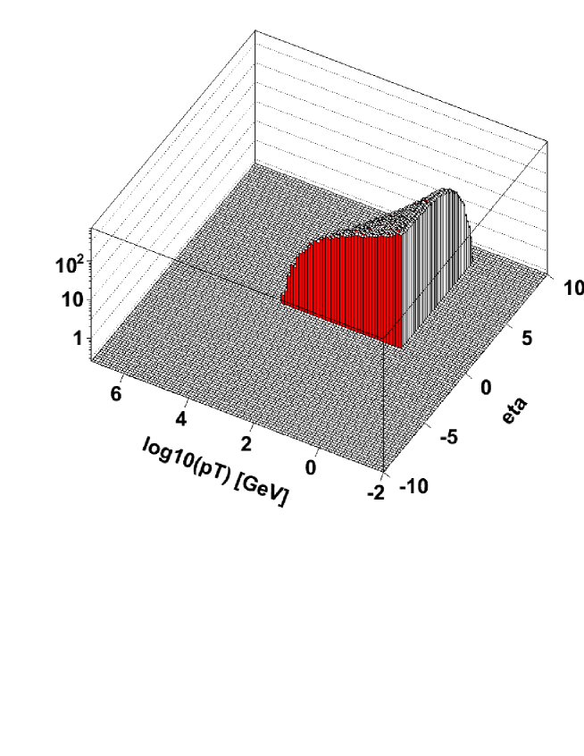
Figure 5: The distribution of rapidity and log of $k^{T}$ from CMC for $2E_{h}=1000$ GeV, $\lambda=1$ GeV and the kernel type (C); pure bremsstrahlung case.

With all the above formalism at hand, we can formulate our CMC algorithm similarly as in the general LL DGLAP case:

• Generate super-level variables $n$, $t_{i}$ $x^{\prime}_{i}$ and $x_{i}$ with the help of the general-purpose MC tool FOAM according to eq. (91), and neglecting $W=\prod W^{G}_{i}$. The parton types $f_{i},i=0,1,2,3...,n-1$ are determined from $f=f_{n}$ according to prescription of ref. [8].

• In the above, the number of flavour transitions ($G\to Q$ and $Q\to G$) is limited to $n=0,1,2,3,4$, aiming at the precision of $\sim 0.2\%$.

• For each $i$-th pure gluon bremsstrahlung segment the emissions variables are generated using the dedicated bremsstrahlung CMC of section 4, according to eq. (93). The weights $W^{G}_{i}$ are calculated.

• Generated MC events are weighted with $W=\prod W^{G}_{i}$. They are optionally turned into weight=1 events using the conventional rejection method.

• The four-momenta $k_{i}^{\mu}$ and $q_{i}^{\mu}$ are reconstructed out of evolution variables and azimuthal angles.

The above algorithm is already implemented in the form of a program in C++ and tested using upgraded version of the Markovian MC of refs. [28] and [17]. The numerical results are documented in the following section.

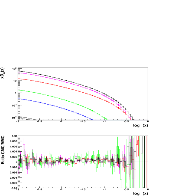
Figure 6: The gluon distribution from CMC and MMC for evolution with the kernel (C’), $\lambda=1$ GeV and $e^{t_{\max}}=2E_{h}=1$ TeV. Contributions from fixed number of the quark gluon transitions $n=0,1,2,3,4$ are also shown. The ratios CMC/MMC in the lower plot are given separately for the total result and for the number of quark gluon transition $n=0,1,2$. The MC statistics is $4.5\cdot 10^{9}$ weighted events for CMC and $10^{10}$ for MMC.

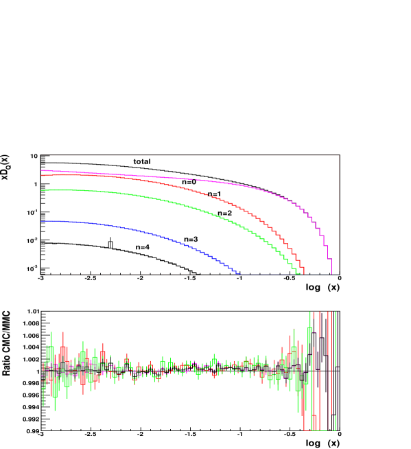
Figure 7: The Quark distribution from CMC and MMC for evolution with the kernel (C’), $\lambda=1$ GeV and $e^{t_{\max}}=2E_{h}=1$ TeV. Contributions from fixed number of the quark gluon transitions $n=0,1,2,3,4$ are also shown. The ratios CMC/MMC in the lower plot are given separately for the total result and for the number of quark gluon transition $n=0,1,2$. The MC statistics is $10^{10}$ weighted events for both CMC and MMC.

6 Numerical tests

Most of the numerical tests proving that the new CMCs of this paper work correctly were done by means of comparison with the updated version of the Markovian MC program MMC [15], which is a descendant of that described in refs. [17, 28]. The version of MMC used below implements exactly the same type evolution with exactly the same kernels and boundary conditions. We can therefore expect numerical agreement of CMC and MMC to within statistical MC error, which will be of the order of $10^{-3}$, for about $10^{10}$ MC events (and for about $10^{2}$ different values of $x$ in a single MC run).

We start, however, with the simple tests in which we verify the correctness of the mapping of the evolution variables into four-momenta. In Fig. 5 the distribution of rapidity and $k^{T}_{i}$ of the emitted gluons is shown. Sharp cut-offs corresponding to the minimum rapidity $\eta\geqslant 0$ (maximum $t$) and minimum $k^{T}\geqslant 1$ GeV are clearly visible in the plot. Note that this plot shows the same triangular area of the logarithmic Sudakov plane as in Fig. 4(a), but now populated with the MC events.

Figure 8: The distributions of $\tau_{i}$ and $x_{i}$ and the emission multiplicity from the CMC and MMC programs. The results are from the MC run for gluon in proton.

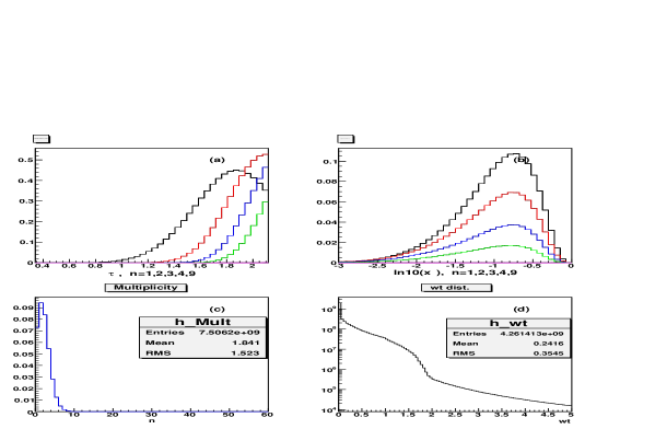
Figure 9: The distributions of $\tau_{i}$ and $x_{i}$ and the emission multiplicity from the CMC and MMC programs. The results are from the MC run for quark in proton.

6.1 Testing CMC versus MMC

We examine results of the evolution from the initial energy scale $\lambda=1$ GeV up to final energy scale of $E_{h}=1$ TeV, using exactly the same initial quark and gluon distributions in a proton at the $Q_{0}=e^{t_{0}}=\lambda=1$ GeV scale as in ref. [8] (they were also used in ref. [28]).

In Fig. 6 the distributions of gluons at $E_{h}=1$ TeV are shown, while in Fig. 7 the corresponding results for quarks, $Q=q+\bar{q}$, are exposed, also at the same high energy scale $E_{h}=1$ TeV. Numerical results are provided for the evolution type (C’) (see section 3.2), that is for $\alpha_{S}(k^{T})$ and the evolution time being identical with the rapidity of the emitted particle. In these two figures we compare the gluon and quark distributions obtained from the current CMC program and from the updated MMC program [15]. The principal numerical results from both programs, marked as “total” in the upper plot of both figures, are indistinguishable. We therefore plot their ratio in the lower plot of both figures. The parton distributions from the CMC and MMC programs agree perfectly, within the statistical errors of $\sim 10^{-3}$ in the entire range of $x$. In the same plots we include individual contributions from a fixed number of the quark gluon transitions $n=0,1,2,3,4$, and their ratios. Again very good agreement between CMC and MMC results is seen.

It should be stressed that the MMC program has been tested numerically at the same $\sim 10^{-3}$ precision level for all types of the kernels (A–C) by comparison with the semi-analytical (non-MC) program APCheb [29]. In addition, for the DGLAP case, MMC was also successfully compared with another non-MC program QCDNum16 [30]. These dedicated tests of MMC using non-MC programs will be published separately in the forthcoming paper [15].

Additionally, in Figs. 8 and 9, we show comparisons of selected (semi-)exclusive distributions from CMC and MMC, i.e. we have chosen for the test the distributions of the consecutive evolution time variables $\tau_{i}(t_{i})$, the energy fractions $x_{i}$ and the total parton emission multiplicity from both CMC and MMC. The above distributions resulting from separate CMC and MMC runs are interposed – no visible difference is seen within the resolution of the plots. The above plots are for a final parton being a gluon in Fig. 8 and a quark in Fig. 9. In these plots one is testing a nontrivial aspect of the CMC algorithm related to removing and restoring the $t$-ordering described in section 4.2. In fact, any departure from the pairwise ordering procedure described in section 4.2 would ruin the agreement of CMC and MMC seen in Figs. 8 and 9! The weight distribution from CMC is also shown in the lower part of these figures.

All the above tests were done for the most interesting case of CMC with the kernel (C). What about numerical tests for cases (A) and (B)? In ref.[8] numerical agreement within $\sim 10^{-3}$ statistical error between CMC and MMC for the LL DGLAP case (A) was already documented. While preparing this work, we have compared CMC and MMC for case (B), $\alpha_{S}(e^{-t}\lambda)$, obtaining equally good numerical agreement. The corresponding plots look quite similar to these in Fig. 6 and Fig. 7.

7 Discussions and summary

We have generalized the constrained Monte Carlo algorithm of ref. [8] from DGLAP to two other more complicated types of the evolution equations, one of them fully compatible with the CCFM evolution equation [12]. The above extentions of the CMC algorithm are implemented in the computer program CMC, tested by comparisons it with the Markovian MC, which also solves exactly the same evolution equations.

Let us point out that the most complicated version (C) of the evolution equation elaborated in this work follows closely the CCFM model as formulated in [25] (except for the temporarily omitted non-Sudakov form-factors). Its Markovian MC implementation SMALLX was worked out in refs. [23, 24], and later on exploited in the construction of the CASCADE MC of ref. [31], which is based on the backward evolution algorithm [7]. Our CMC program was tested against our own Markovian MC, see previous section. However, it would be interesting to compare it also with the above SMALLX and CASCADE programs. We hope this will be done in the near future.

Since the CMC program of this work will be used as a building block in the MC event generator for the Drell–Yan type processes and deep inelastic lepton-hadron scattering, the explicit mapping of the evolution variables into four-momenta of the emitted particles is also defined, implemented and tested. The evolution time is mapped into the rapidity variable (angular ordering). A sharp cut-off is imposed on the $k^{T}$ and rapidity of the emitted particle. The sharp cut-off in the rapidity will be useful when combining two CMCs for two colliding initial state hadrons, with neither gaps nor overlaps in the emission phase space.

The CMC algorithm was worked out in detail and tested for three types of the evolution kernels and the phase–space limits. It was purposely defined/described in such a way that it can be easily generalized to other types of the evolution kernels. In the following works it will be used as a component in the MC modelling of the initial state parton shower for showering of a single hadron in a more complete MC project for LHC.

Acknowledgments
We would like to thank K. Golec-Biernat for the useful help and discussions. We acknowledge the warm hospitality of the CERN Physics Department, where part of this work was done.

Appendix

Appendix A Auxiliary functions in form-factors

A.1 Triangle function $\varrho$

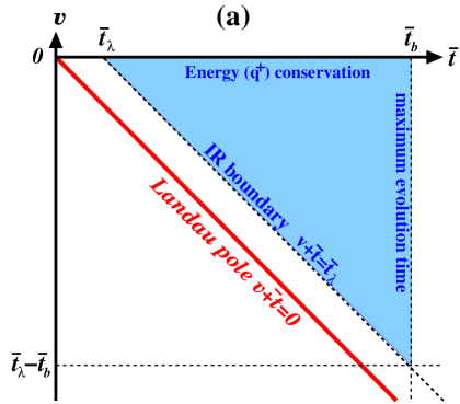
Figure 10: The integration area in the definition of the functions: (a) $\varrho({\bar{t}}_{b};{\bar{t}_{\lambda}})$ and (b) $\varrho({\bar{t}}_{b}+v_{x};{\bar{t}_{\lambda}})$.

The simplest component function in the Sudakov formactor in cases (B) and (C) of $z$-dependent $\alpha_{S}$ reads as follows

$$\varrho({\bar{t}}_{b};{\bar{t}_{\lambda}})=\int^{{\bar{t}}_{b}}d{\bar{t}}\int^{0}dv\;\frac{\theta_{{\bar{t}}+v>t_{\lambda}}}{{\bar{t}}+v}=\theta_{{\bar{t}}_{b}>{\bar{t}}_{\lambda}}\{{\bar{t}}_{b}\;[\ln{\bar{t}}_{b}-\ln{\bar{t}}_{\lambda}-1]+{\bar{t}}_{\lambda}\},$$ (97)

where $\lambda$ defines the IR cut-off. Here and in the following, we follow certain notation rules allowing us to write the above and similar functions in a compact way:

1. For all variables like $t$, $t_{b}$ and $t_{\lambda}$ bar over them means ${\bar{t}}=t-\ln\Lambda_{0}$, ${\bar{t}}_{b}=t_{b}-\ln\Lambda_{0}$, ${\bar{t}}_{\lambda}=t_{\lambda}-\ln\Lambda_{0}$, etc., where $\Lambda_{0}$ is that in eq. (26), i.e. the position of the Landau pole.

2. Occasionally we shall omit the explicit dependence on $t_{\lambda}=\ln\lambda$, that is we always understand $\varrho({\bar{t}}_{b})\equiv\varrho({\bar{t}}_{b};{\bar{t}_{\lambda}})$.

3. We always understand that $\int_{a}^{b}dx\equiv 0$ when $b\leq a$.

The area of the integration in eq. (97) is the triangle, depicted if Fig. 10 (a).

The following similar integral, with the same integrand, but slightly different triangular integration area, depicted in Fig. 10 (b), can be expressed using the same function $\varrho$:

$$\int^{{\bar{t}}_{b}}d{\bar{t}}\int^{v_{x}}dv\frac{\theta_{{\bar{t}}+v>\bar{t}_{\lambda}}}{{\bar{t}}+v}=\varrho({\bar{t}}_{b}+v_{x};{\bar{t}_{\lambda}}).$$ (98)

A.2 Trapezoid function $\varrho_{2}$

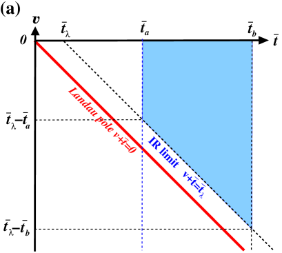
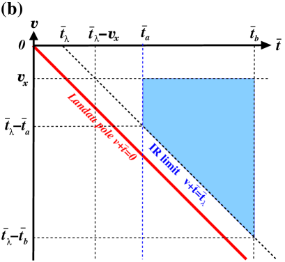
Figure 11: The integration area in the functions: (a) $\varrho_{2}({\bar{t}}_{a},{\bar{t}}_{b};{\bar{t}_{\lambda}})$ and (b) $\varrho_{2}({\bar{t}}_{a}+v_{x},{\bar{t}}_{b}+v_{x};{\bar{t}_{\lambda}})$.

The other basic IR-singular component function in the Sudakov form-factor reads

$$\varrho_{2}({\bar{t}}_{a},{\bar{t}}_{b};{\bar{t}_{\lambda}})=\int^{{\bar{t}}_{b}}_{{\bar{t}}_{a}}d{\bar{t}}\int^{0}dv\frac{\theta_{{\bar{t}}+v>\bar{t}_{\lambda}}}{{\bar{t}}+v}=\theta_{{\bar{t}}_{b}>{\bar{t}}_{a}}\{\varrho({\bar{t}}_{b};{\bar{t}_{\lambda}})-\varrho({\bar{t}}_{a};{\bar{t}_{\lambda}})\}$$ (99)

The corresponding integration area is the trapezoid depicted in Fig. 11 (a). The above calculation result is obvious if one notices that the trapezoid is the difference of two overlapping triangles. Similarly, the following integral with the trapezoid integration area of Fig. 11 (a) is again expressed in terms of the functions already defined above

$$\begin{split}\varrho^{[1]}_{2}(v_{x},{\bar{t}}_{a},{\bar{t}}_{b};{\bar{t}_{\lambda}})&=\int^{{\bar{t}}_{b}}_{{\bar{t}}_{a}}d{\bar{t}}\int^{v_{x}}dv\frac{\theta_{{\bar{t}}+v>\bar{t}_{\lambda}}}{{\bar{t}}+v}\\ &=\theta_{{\bar{t}}_{b}>{\bar{t}}_{a}}\{\varrho({\bar{t}}_{a}+v_{x};{\bar{t}_{\lambda}})-\varrho({\bar{t}}_{b}+v_{x};{\bar{t}_{\lambda}})\}=\varrho_{2}({\bar{t}}_{a}+v_{x},{\bar{t}}_{b}+v_{x};{\bar{t}_{\lambda}}).\end{split}$$ (100)

Let us stress that keeping $\theta_{{\bar{t}}_{b}>{\bar{t}}_{\lambda}}$ in the basic function $\varrho$ of eq. (97) is essential for validity of the evaluation of all the following related functions and integrals.

A.3 Non-singular functions and mapping

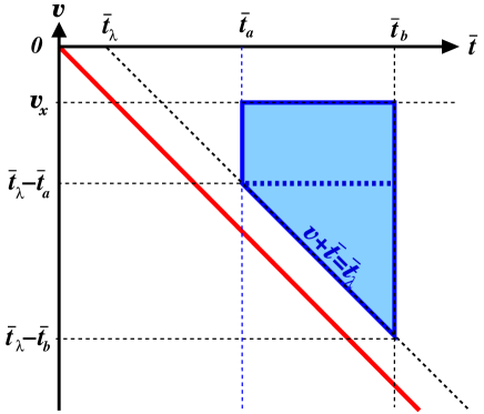
Figure 12: The integration area in the function $\varrho^{[F]}_{2}({\bar{t}}_{a},{\bar{t}}_{b},v_{x};{\bar{t}_{\lambda}})$.

Let us evaluate now the following integral, which is similar to $\varrho_{2}$, except that we insert into the integrand the additional function $F(v,t)$:

$$\varrho^{[F]}_{2}(v_{x},{\bar{t}}_{a},{\bar{t}}_{b};{\bar{t}_{\lambda}})=\int^{{\bar{t}}_{b}}_{{\bar{t}}_{a}}d{\bar{t}}\int^{v_{x}}dv\;\frac{\theta_{{\bar{t}}+v>\bar{t}_{\lambda}}}{{\bar{t}}+v}F(v,{\bar{t}}).$$ (101)

Of course, for $F=1$ we recover $\varrho_{2}$. However, even in this case the following evaluation of $\varrho^{[F]}_{2}$ will be interesting, because we shall swap the integration order and introduce variable mapping, exactly the same as we have used for finding out $K(v)$ and eliminating $K(v)$ through the additional mapping $r(v)$. Such a swapping integration order is also used for evaluation of the non-IR part of the bremsstrahlung integral and flavour changing contributions, where we have $F(v,t)=F(v)$, hence the inner integration over ${\bar{t}}$ can be done analytically and the outer one over $v$ is done numerically.

In a general case, after swapping the integration order

$$\varrho^{[F]}_{2}(v_{x},{\bar{t}}_{a},{\bar{t}}_{b};{\bar{t}_{\lambda}})=\int\limits_{{\bar{t}}_{\lambda}-{\bar{t}}_{b}}^{v_{x}}dv\Bigg{\{}\theta_{v_{x}<{\bar{t}}_{\lambda}-{\bar{t}}_{a}}\int\limits_{{\bar{t}}_{\lambda}-v_{x}}^{{\bar{t}}_{b}}d{\bar{t}}\;\frac{1}{{\bar{t}}+v}+\theta_{v_{x}>{\bar{t}}_{\lambda}-{\bar{t}}_{a}}\int\limits_{{\bar{t}}_{a}}^{{\bar{t}}_{b}}d{\bar{t}}\;\frac{1}{{\bar{t}}+v}\Bigg{\}}F(v,{\bar{t}})$$ (102)

the integration is split into two parts, first for the triangle and second for the rectangle integration area, see Fig. 12 for illustration. The above change of the integration order was also exploited by the authors of HERWIG MC [5, 32]. The internal integral can be transformed using the identities:

$$\begin{split}&\varrho^{\prime}({\bar{t}}_{b})=\partial_{{\bar{t}}_{b}}\varrho({\bar{t}}_{b};{\bar{t}}_{\lambda})=\int\limits_{{\bar{t}}_{\lambda}-{\bar{t}}_{b}}^{0}dv\;\frac{1}{{\bar{t}}+v}=\theta_{{\bar{t}}_{b}>{\bar{t}}_{\lambda}}(\ln{\bar{t}}_{b}-\ln{\bar{t}}_{\lambda}),\\ &\varrho^{\prime[1]}_{2}(v_{x},{\bar{t}}_{a},{\bar{t}}_{b})=\partial_{v_{x}}\varrho^{[1]}_{2}(v_{x},{\bar{t}}_{a},{\bar{t}}_{b};{\bar{t}_{\lambda}})\\ &~{}~{}~{}~{}~{}~{}~{}~{}~{}~{}~{}=\theta_{v_{x}>{\bar{t}}_{\lambda}-{\bar{t}}_{a}}[\varrho^{\prime}({\bar{t}}_{b}+v_{x})-\varrho^{\prime}({\bar{t}}_{a}+v_{x})]+\theta_{v_{x}<{\bar{t}}_{\lambda}-{\bar{t}}_{a}}\varrho^{\prime}({\bar{t}}_{b}+v_{x}),\end{split}$$ (103)

to the following convenient form

$$\begin{split}\varrho^{[F]}_{2}(v_{x},{\bar{t}}_{a},{\bar{t}}_{b};{\bar{t}_{\lambda}})&=\int\limits_{{\bar{t}}_{\lambda}-{\bar{t}}_{b}}^{v_{x}}dv\;\varrho^{\prime[1]}_{2}(v,{\bar{t}}_{a},{\bar{t}}_{b})\int\limits_{0}^{1}d\left(\frac{\ln({\bar{t}}+v)}{\varrho^{\prime[1]}_{2}(v,{\bar{t}}_{a},{\bar{t}}_{b})}\right)F(v,{\bar{t}})\\ &=\varrho^{\prime[1]}_{2}(v_{x},{\bar{t}}_{a},{\bar{t}}_{b})\int\limits_{0}^{1}d\xi(v)\int\limits_{0}^{1}d\sigma(v,{\bar{t}})\;F(v,{\bar{t}}),\end{split}$$ (104)

where

$$\xi(v)=\frac{\varrho^{[1]}_{2}(v,{\bar{t}}_{a},{\bar{t}}_{b})}{\varrho^{[1]}_{2}(v_{x},{\bar{t}}_{a},{\bar{t}}_{b})},\quad\sigma(v,{\bar{t}})=\frac{\ln({\bar{t}}+v)}{\varrho^{\prime[1]}_{2}(v,{\bar{t}}_{a},{\bar{t}}_{b})}.$$ (105)

The above mapping is used in the bremsstrahlung CMC in cases (B) and (C). In this context one also needs to perform the inverse mapping $v(\xi)$, which requires numerical inversion of $\varrho^{[1]}_{2}(v,{\bar{t}}_{a},{\bar{t}}_{b})$ as a function of $v$. Once $v$ is known, the second inverse mapping $t(\sigma,\xi)$ is easily implemented, as it can be formulated in a fully analytical form. As already indicated, a very similar variant of the above integration order is used in the evaluation of the non-IR and flavour-changing parts of the Sudakov form-factor.

A.4 Integration area in the plane of $\ln k^{T}$ and rapidity $\eta$

Finally, let us relate the phase space $v$ and $t$ used in the calculation of the form-factor above with the Sudakov plane in $\ln k^{T}$ and the rapidity $\eta$. This is done in the pictorial way in Fig. 4, where we depict a situation with three emission, underlining the trapezoid integration domain for the Sudakov function $\Phi(t_{3},t_{2}|x_{2})$. This is show on the right hand side of the figure, as the trapezoid marked by $abcd$, in the plane of $t$ and $v$. On the left hand side of this figure, the corresponding trapezoid is seen in the plane of $\ln k^{T}$ and rapidity $\eta$. Let us remind the reader that in the case (C) we define $v_{i}=\ln y_{i}=\ln(x_{i}-x_{i-1})$ and the rapidities $\eta_{i}$ are related to the evolution times $t_{i}$ with the simple linear transformation of eq. (21) in Sec. 3.1.

References

• [1] J. C. Collins, D. E. Soper, and G. Sterman, Nucl. Phys. B250 (1985) 199.
• [2] G. T. Bodwin, Phys. Rev. D31 (1985) 2616.
• [3] R. Ellis, W. Stirling, and B. Webber, QCD and Collider Physics. Cambridge University Press, 1996.
• [4] T. Sjostrand et al., Comput. Phys. Commun. 135 (2001) 238–259, hep-ph/0010017.
• [5] G. Corcella et al., JHEP 01 (2001) 010, hep-ph/0011363.
• [6] S. Jadach et al., in preparation.
• [7] T. Sjostrand, Phys. Lett. B157 (1985) 321.
• [8] S. Jadach and M. Skrzypek, Comput. Phys. Commun. 175 (2006) 511–527, hep-ph/0504263.
• [9] S. Jadach and M. Skrzypek, Acta Phys. Polon. B36 (2005) 2979–3022, hep-ph/0504205.
• [10] S. Jadach and M. Skrzypek, Report CERN-PH-TH/2005-146, IFJPAN-V-05-09, Contribution to the HERA–LHC Workshop, CERN–DESY, 2004–2005, http://www.desy.de/$\sim$heralhc/, hep-ph/0509178.
• [11] L.N. Lipatov, Sov. J. Nucl. Phys. 20 (1975) 95;
V.N. Gribov and L.N. Lipatov, Sov. J. Nucl. Phys. 15 (1972) 438;
G. Altarelli and G. Parisi, Nucl. Phys. 126 (1977) 298;
Yu. L. Dokshitzer, Sov. Phys. JETP 46 (1977) 64.
• [12] M. Ciafaloni, Nucl. Phys. B296 (1988) 49;
S. Catani, F. Fiorani and G. Marchesini, Phys. Lett. B234 339, Nucl. Phys. B336 (1990) 18;
G. Marchesini, Nucl. Phys. B445 (1995) 49.
• [13] S. Frixione and B. R. Webber, JHEP 06 (2002) 029, hep-ph/0204244.
• [14] S. Frixione and B. R. Webber, hep-ph/0601192.
• [15] S. Jadach et al., in preparation.
• [16] S. Jadach, M. Skrzypek, and Z. Was, hep-ph/0701174.
• [17] K. Golec-Biernat, S. Jadach, W. Placzek, and M. Skrzypek, Acta Phys. Polon. B37 (2006) 1785–1832, hep-ph/0603031.
• [18] J. C. Collins and D. E. Soper, Nucl. Phys. B193 (1981) 381.
• [19] G. Curci, W. Furmanski, and R. Petronzio, Nucl. Phys. B175 (1980) 27.
• [20] A. H. Mueller, Phys. Lett. B104 (1981) 161–164.
• [21] S. Catani, B. R. Webber, and G. Marchesini, Nucl. Phys. B349 (1991) 635–654.
• [22] Y. Dokshitzer, V. Khoze, A. Mueller, and S. Troyan, Basics of Perturbative QCD. Editions Frontieres, 1991.
• [23] G. Marchesini and B. R. Webber, Nucl. Phys. B349 (1991) 617–634.
• [24] G. Marchesini and B. R. Webber, Nucl. Phys. B349 (1991) 617–634.
• [25] G. Marchesini, Nucl. Phys. B445 (1995) 49–80, hep-ph/9412327.
• [26] D. Amati, A. Bassetto, M. Ciafaloni, G. Marchesini, and G. Veneziano, Nucl. Phys. B173 (1980) 429.
• [27] S. Jadach, Comput. Phys. Commun. 152 (2003) 55–100, physics/0203033.
• [28] S. Jadach and M. Skrzypek, Acta Phys. Polon. B35 (2004) 745–756, hep-ph/0312355.
• [29] K. Golec-Biernat, the Fortran code to be obtained from the author, unpublished.
• [30] M. Botje, ZEUS Note 97-066, http://www.nikhef.nl/ h24/qcdcode/.
• [31] H. Jung and G. P. Salam, Eur. Phys. J. C19 (2001) 351–360, hep-ph/0012143.
• [32] G. Marchesini and B. R. Webber, Nucl. Phys. B310 (1988) 461.