On Higgs mass generation mechanism in the Standard Model

Abstract

The mass-generation mechanism is the most urgent problem of the modern particle physics. The discovery and study of the Higgs boson with the Large Hadron Collider at CERN are the highest priority steps to solve the problem. In this paper, the Standard Model Higgs mechanism of the elementary particle mass generation is reviewed with pedagogical details. The discussion of the Higgs quadric self-coupling $\lambda$ parameter and the bounds to the Higgs boson mass are presented. In particular, the unitarity, triviality, and stability constraints on the Higgs boson mass are discussed. The generation of the finite value for the $\lambda$ parameter due to quantum corrections via effective potential is illustrated. Some simple predictions for the top quark and the Higgs boson masses are given when both the top Yukawa coupling and the Higgs self-coupling $\lambda$ are equal to 1.

I Introduction

One of the highest priorities of particle physics today is the discovery of the dynamics responsible for Electro-Weak Symmetry Breaking (EWSB) Haber:2004tm . In the Standard Model, nowadays the main working paradigm of particle theory, this dynamics is expected due to self-interactions of special complex scalar fields. This approach predicts the existence of one physical elementary scalar, the so-called Higgs boson Gunion:1989we ; Gunion:1992hs . A search for and the discovery of this still-escaping boson, and investigation of its properties are practical steps to solve the problem of EWSB which are currently planned to perform with the Large Hadron Collider (LHC) and in future with the International Linear Collider (ILC).

The modern Standard Model (SM) of particle physics is a unified framework to describe electromagnetic and weak interactions between quarks and leptons together with strong interactions between quarks (see, for example, Djouadi:2005gi ). It is the Yang-Mills theory based on the electroweak symmetry group SU(2)${}_{\rm L}\times$U(1)_Y of Glashow, Weinberg, and Salam Glashow:1961tr ; Weinberg:1967tq ; Salam:1969aa and strong SU(3)_C group of QCD Gell-Mann:1964nj ; Fritzsch:1973pi ; Gross:1973id ; Politzer:1973fx . This model (before the electroweak symmetry breaking) has only matter and gauge fields. The matter fields are composed of three generations of fermions (spin-1/2), left-handed and right-handed quarks and leptons, $\displaystyle f_{\rm L,R}=\frac{1\mp\gamma_{5}}{2}f$. It is crucial for our consideration that the left-handed fermions are in the weak SU(2)_L isodoublets, while the right-handed fermions are weak isosinglets. Moreover, both left- and right-handed quarks are triplets under the ${\rm SU(3)_{C}}$ group, while all leptons are color singlets. The gauge fields mediate the above-mentioned interactions and correspond to the (spin-1) bosons. In the electroweak sector, the field $B_{\mu}$ corresponds to the U(1)_Y group and the three fields $W^{1,2,3}_{\mu}$ correspond to the SU(2)_L group. There is also an octet of gluon fields $G_{\mu}^{a}$ which correspond to the color ${\rm SU(3)_{C}}$ group. Due to the non-Abelian nature of the SU(2) and SU(3) groups, there are triple and quartic self-interactions between their gauge fields $V_{\mu}=W_{\mu}$ or $G_{\mu}$. The matter fields $\psi$ are minimally coupled to the gauge fields through the covariant derivative $D_{\mu}$ (see Appendix VI.1), which leads to a unique form of interaction between the fermion and gauge fields, ($-g_{i}\overline{\psi}V_{\mu}\gamma^{\mu}\psi$), where $g_{s}$, $g_{2}$, and $g_{1}$ are, respectively, the coupling constants of ${\rm SU(3)_{C}}$, ${\rm SU(2)_{L}}$, and ${\rm U(1)_{Y}}$.

The SM Lagrangian, without mass terms for fermions and gauge bosons, is then given by

$${\cal L}_{\rm SM} = -\frac{1}{4}G_{\mu\nu}^{a}G^{\mu\nu}_{a}-\frac{1}{4}W_{\mu\nu}^{a}W^{\mu\nu}_{a}-\frac{1}{4}B_{\mu\nu}B^{\mu\nu}$$

$$+\bar{L_{i}}\,iD_{\mu}\gamma^{\mu}\,L_{i}+\bar{e}_{Ri}\,iD_{\mu}\gamma^{\mu}\,e_{R_{i}}\ +\bar{Q_{i}}\,iD_{\mu}\gamma^{\mu}\,Q_{i}+\bar{u}_{Ri}\,iD_{\mu}\gamma^{\mu}\,u_{R_{i}}\ +\bar{d}_{Ri}\,iD_{\mu}\gamma^{\mu}\,d_{R_{i}}.$$

This Lagrangian is invariant under local ${\rm SU(3)_{C}\times SU(2)_{L}\times U(1)_{Y}}$ gauge transformations for fermion and gauge fields. Here $L_{i}$ and $Q_{i}$ denote the left-handed lepton and quark doublets, respectively, while $f_{R}$ denotes the relevant right-handed singlets. In the case of the electroweak sector, for instance, one has the gauge transformations:

$$L(x)\to L^{\prime}(x)=e^{i\alpha_{a}(x)T^{a}+i\beta(x)Y}L(x)\ \ ,\ \ R(x)\to R^{\prime}(x)=e^{i\beta(x)Y}R(x)$$

$$\vec{W}_{\mu}(x)\to\vec{W_{\mu}}(x)-\frac{1}{g_{2}}\partial_{\mu}\vec{\alpha}(x)-\vec{\alpha}(x)\times\vec{W}_{\mu}(x)\ ,\ B_{\mu}(x)\to B_{\mu}(x)-\frac{1}{g_{1}}\partial_{\mu}\beta(x).$$ (2)

The gauge fields and the fermion fields are massless here. More details one can find in Appendix VI.1.

It is interesting to note that in the case of strong interactions (while the gluons are indeed massless particles) the mass terms of the form $-m_{q}\overline{\psi}\psi$ can be generated for the colored quarks in an SU(3) gauge invariant way. This is due to the fact that all (left- and right-handed) quarks belong only to triplets of the SU(3) color group and all transform in the same manner.

On the contrary, the situation in the electroweak sector is really horrible. Indeed, one knows experimentally that the weak gauge bosons are massive and the weak interaction is very short ranged. However, as soon as one adds standard mass terms for the gauge bosons, $\frac{1}{2}M_{W}^{2}W_{\mu}W^{\mu}$, one immediately violates the local SU(2)$\times$U(1) gauge invariance. This is clearly seen for the QED where the photon is massless because of the U(1) local gauge symmetry. Indeed, the transfromed “photon” mass term

$$\frac{1}{2}M_{\gamma}^{2}A_{\mu}A^{\mu}\to\frac{1}{2}M_{\gamma}^{2}(A_{\mu}-\frac{1}{e}\partial_{\mu}\alpha)(A^{\mu}-\frac{1}{e}\partial^{\mu}\alpha)\neq\frac{1}{2}M_{\gamma}^{2}A_{\mu}A^{\mu}$$ (3)

can hold its form untouched only if $M_{\gamma}^{2}\equiv 0$. In addition, if one includes explicitly the mass term $-m_{f}\overline{\psi}_{f}\psi_{f}$ for the SM fermion $f$ in the Lagrangian, then, for instance, one would have for the electron

$$-m_{e}\bar{e}e\equiv-m_{e}\bar{e}\bigg{(}\frac{1-\gamma_{5}}{2}+\frac{1+\gamma_{5}}{2}\bigg{)}e=-m_{e}(\bar{e}_{R}e_{L}+\bar{e}_{L}e_{R})$$ (4)

which is obviously noninvariant under the weak isospin symmetry transformations discussed above, since $e_{L}$ is a member of the SU(2)_L doublet, while $e_{R}$ is the SU(2)_L singlet and, therefore, they change under transformation in a different manner.

Therefore, the mass terms for gauge bosons and fermions induced “by-hand” lead to an obvious breakdown of the local ${\rm SU(2)_{L}\times U(1)_{Y}}$ gauge invariance. The unbroken symmetry means that all fundamental particles have to be massless. This is because both the fermion mass term $f_{L}\times f_{R}$ and that of gauge bosons are not SU(2)_L invariant Kazakov:1989ny . One can see, that generation of the mass for an elementary particle in the SM is strongly connected with the symmetry violation. One needs a mechanism for this violation, and one believes, that this mechanism will simultaneously allow the elementary particles to obtian their masses.

In principle, the idea of mass generation due to interaction is rather simple. Consider the renormalizable Lagrangian ${\cal L}=gA_{\mu}A_{\mu}\phi$ describing interaction of the scalar field $\phi$ with the massless vector field $A_{\mu}$. In an ordinary theory mean vacuum expectation values (vev’s) are zero. Assume now that the scalar field has nonvanishing vev $v\neq 0$, so $\phi=v+\sigma$ with $\langle 0|\sigma|0\rangle=0$. The Lagrangian becomes ${\cal L}=gvA_{\mu}A_{\mu}+gA_{\mu}A_{\mu}\sigma$. The first term is a right mass term and the vector particle obtains a mass $m^{2}=2vg$. The only question is where $v\neq 0$ comes from? Gaillard:1977wu . In other words, is there a way to generate the gauge boson and the fermion masses without violating SU(2)$\times$U(1) gauge invariance? The positive answer is given by Higgs, Kibble and others Higgs:1964pj ; Higgs:1966ev ; Kibble:1967sv . This is the spontaneous symmetry breaking Higgs mechanism (see Djouadi:2005gi and Appendix VI.1).

In fact, the Higgs mechanism is needed due to the SU(2)$\times$U(1) gauge structure of the SM. It is remarkable that from the practical point of view the mass generation by means of the Higgs mechanism in the SM is forced by the $V$–$A$ structure of the weak interaction (and in some sense by the absence of the right-handed neutrinos $\nu_{R}$ or even by the masslessness of all neutrinos).

Below, in discussing the Higgs mechanism and related topics we follow, to a large extent, the excellent review of A. Djouadi Djouadi:2005gi .

II Higgs Mechanisms

II.1 The simplest example

First of all, consider a simple Lagrangian for a scalar real field $\phi$

$${\cal L}=\frac{1}{2}\partial_{\mu}\phi\,\partial^{\mu}\phi-V(\phi),\qquad{\rm where}\qquad V(\phi)=\frac{1}{2}\mu^{2}\phi^{2}+\frac{1}{4}\lambda\phi^{4}.$$ (5)

Since the potential should be bounded from below, the self-coupling $\lambda>0$. With the mass term $\mu^{2}>0$, the potential $V(\phi)$ is always positive. Furthermore, the $\phi^{4}$-term describes self-interaction with intensity $\lambda$. Other terms $\phi^{n}$ with $n>4$ have to be excluded from consideration because they produce infinities in calculated observables Kane:1987gb . The case when the potential $V(\phi)$ also contains an extra $\phi^{3}$-term is considered in Appendix VI.2.

To find an excitation spectrum of the system described by Lagrangian (5), one first has to find minimum (or minima) of the potential $V(\phi)$. The system has minimal energy when its both kinetic and potential energies separately are minimal. The kinetic energy is minimal when $\phi$ is a constant. The minimum gives one a classical main (vacuum) state of the system. Next, one has to decompose the field $\phi$ in the vicinity of this main state and has to find excitation states. In a field theory the main state is the vacuum and the excitations are particles. Particle masses are defined by the form of the Lagrangian in the vicinity of the classical minimum Kane:1987gb . When $\mu^{2}>0$ (left panel in Fig. 1), the minimum of potential (5) is reached at $\phi=0$. Therefore, vacuum expectation value for the field $\langle 0|\phi|0\rangle\equiv\phi_{0}=0$. Lagrangian (5) then simply describes a spin-zero particle of mass $\mu$. It is also invariant under the reflexion symmetry $\phi\to-\phi$ since there are no cubic terms.

Figure 1: The potential $V$ of the scalar field $\phi$ in the case $\mu^{2}>0$ (left) and $\mu^{2}<0$ (right). From Djouadi:2005gi .

If $\mu^{2}<0$ (right panel in Fig. 1), the potential $V(\phi)$ has minima not at $\phi_{0}=0$ but at $\phi_{1}$ and $\phi_{2}$ which solve the minimum condition  $\partial V/\partial\phi=\phi(\mu^{2}+\lambda\phi^{2})=0$. Now the system has two states (vacuums) with the lowerst energy $\displaystyle V_{\min}=-\frac{v^{4}\lambda}{4}<0$  at

$$\phi_{1}=\sqrt{-\frac{\mu^{2}}{\lambda}}\equiv v>0,\quad{\rm and}\quad\phi_{2}=-\sqrt{-\frac{\mu^{2}}{\lambda}}\equiv-v.$$ (6)

The quantities $\phi_{1}\equiv+v$ and $\phi_{2}\equiv-v$ are the vacuum mean values of the field $\phi$ and are also called the vacuum expectation value (vev) of the scalar field $\phi$. Lagrangian (5) no longer describes a particle with mass $\mu$.

To find now energies of the particles (and to interpret correctly the theory), one has to choose one of the minimum, e.g., with $\phi=v$, and investigate the situation in the vicinity of the minimum of the potential $V(\phi)$. To this end, one introduces a new scalar field $\sigma$ in such a way that $\phi=v+\sigma$ and $\langle 0|\sigma|0\rangle=0$. Furthermore, one has to expand all the terms in Lagrangian (5) in series in the small parameter $\sigma$ around the potential minimum at $\sigma=0$. In terms of the new field $\sigma$, the Lagrangian becomes

$${\cal L} = \frac{1}{2}\partial_{\mu}\sigma\,\partial^{\mu}\sigma-\left\{\frac{\mu^{2}}{2}[v^{2}+2v\sigma+\sigma^{2}]+\frac{\lambda}{4}[v^{4}+4v^{3}\sigma+6v^{2}\sigma^{2}+4v\sigma^{3}+\sigma^{4}]\right\}=$$

$$= \frac{1}{2}\partial_{\mu}\sigma\,\partial^{\mu}\sigma-\left\{\frac{v^{2}}{2}(\mu^{2}+\frac{\lambda v^{2}}{2})+v\sigma(\mu^{2}+\lambda\sigma^{2})+\frac{\sigma^{2}}{2}(\mu^{2}+3v^{2}\lambda)+\lambda v\sigma^{3}+\frac{\lambda}{4}\sigma^{4}\right\}.$$

With the minimum relation $\mu^{2}=-\lambda v^{2}$ the linear term disappears and one finally has

$${\cal L} = \frac{1}{2}\partial_{\mu}\sigma\,\partial^{\mu}\sigma-\frac{2\lambda v^{2}}{2}\sigma^{2}-\lambda v\sigma^{3}-\frac{\lambda}{4}\sigma^{4}+\frac{\lambda v^{4}}{4}.$$ (7)

Due to the correct sign of the $\sigma^{2}$-term one can interpret it as a mass term, thus Lagrangian (7) describes a scalar field of mass $m_{\sigma}^{2}=2\lambda v^{2}=-2\mu^{2}$, with $\sigma^{3}$ and $\sigma^{4}$ being self-interactions. The new mass $m_{\sigma}$ was generated due to self-interactions of the field $\sigma$ Kane:1987gb , and $m^{2}_{\sigma}>|\mu^{2}|$ means that the back-attractive “force” for the new $\sigma$ field would be stronger than for the initial field $\phi$. Since there are now cubic terms, the reflexion symmetry is broken. This is the simplest example of spontaneously broken symmetry. The symmetry is violated by means of inevitable alternative — one must choose only one concrete vacuum (at $\phi_{1}=v$, or at $\phi_{2}=-v$). After that the unique vacuum does not possess the symmetry of the initial Lagrangian (5). Actually, the symmetry transformation turns one vacuum state (with $\phi_{1}=v$) into the other one (with $\phi_{2}=-v$).

The Lagrangian (7) now has the potential with nonzero cubic term,

$$V(\sigma)=\lambda v^{2}\sigma^{2}+\lambda v\sigma^{3}+\frac{\lambda}{4}\sigma^{4}-\frac{\lambda v^{4}}{4}.$$

Due to this term the potential could, in principle, have minimum at $\sigma\neq 0$, which spoils the main condition $\langle 0|\sigma|0\rangle=0$. (See the discussion of the Higgs mechanism with the extra $\phi^{3}$-term in Appendix VI.2.) Applying the extremum condition to this potential one has the relation

$$\frac{\partial V}{\partial\sigma}=\lambda\sigma(\sigma^{2}+3v\sigma+2v^{2})=\lambda\sigma(\sigma+v)(\sigma+2v)=0.$$ (8)

There are 3 extrema with $V(\sigma=0)=-{\lambda v^{4}}/{4}<0$,  $V(\sigma=-v)=\lambda v^{4}(1-1+1/4-1/4)=0$, and $V(\sigma=-2v)=\lambda v^{4}(4-8+16/4-1/4)=V(\sigma=0)=-{\lambda v^{4}}/{4}$. Therefore, two minima have the same depth and we can safely choose as a true vacuum the minimum at $\sigma=0$ which indeed has $\langle 0|\sigma|0\rangle=0$. In fact, it is not surprising that the cubic term does not spoil the vacuum. Moving into only one vacuum state one physically does not introduce any new dynamics. Therefore, there is no reason to change the shape of the potential and it remains unchanged. However, to reproduce the unchanged shape of the potential in the new (shifted) coordinate framework (where $\langle 0|\sigma|0\rangle=0$), one needs right this cubic term.

II.2 The Higgs mechanism with a complex scalar field

The relevant Higgs Lagrangian for a complex scalar field $\phi=\frac{1}{\sqrt{2}}(\phi_{1}+i\phi_{2})$ is

$${\cal L}=\left({\partial_{\mu}\phi}\right)^{*}\left({\partial^{\mu}\phi}\right)-\mu^{2}\phi^{*}\phi-\lambda\left({\phi^{*}\phi}\right)^{2}$$ (9)

with at least $\lambda>0$. This Lagrangian is invariant under global gauge transformations $\phi\to\phi^{\prime}=e^{i\chi}\phi$ and, therefore, has global U(1)-symmetry. When $\mu^{2}<0$ the scalar potential

$$V(\phi) = \mu^{2}\phi^{*}\phi+\lambda(\phi^{*}\phi)^{2}=\frac{\mu^{2}}{2}(\phi_{1}-i\phi_{2})(\phi_{1}+i\phi_{2})+\frac{\lambda}{4}((\phi_{1}-i\phi_{2})(\phi_{1}+i\phi_{2}))^{2}=$$

$$= \frac{\mu^{2}}{2}(\phi^{2}_{1}+\phi^{2}_{2})+\frac{\lambda}{4}(\phi^{2}_{1}+\phi^{2}_{2})^{2}$$

has minimum values of $\displaystyle V(\phi)_{\min}=\frac{\mu^{2}}{2}v^{2}+\frac{\lambda}{4}v^{4}=-\frac{\lambda}{4}v^{4}<0\$ at $\displaystyle\phi^{2}_{0}=\frac{v^{2}}{2}$ along a circle of the radius $v$ in the ($\phi_{1},\phi_{2}$), plane where $v$ is given by

$$v^{2}=\phi^{2}_{1}+\phi^{2}_{2},\qquad v^{2}=\frac{-\mu^{2}}{\lambda}>0.$$ (10)

To construct a theory, one has to investigate the situation in the vicinity of one of the minima in the circle. To this end, one has to choose one of the minima (to violate the symmetry of all possible solutions). One can take the real scalar field $\phi_{1}$ with the nonzero vacuum expectation value $\phi_{1}=v$, while the imaginary one $\phi_{2}=0$ at the minimum. Furthermore, the scalar complex field $\phi$ can be parameterized also in the form (with both real $\eta(x)$ and $\xi(x)$)

$$\phi(x)=\frac{1}{\sqrt{2}}\left(v+\eta(x)+i\xi(x)\right)$$

with $\eta(x)=\xi(x)=0$ at $V(\phi)_{\min}$. Therefore, after introduction of a Higgs mass

$$M_{h}=\sqrt{2\lambda v^{2}}\equiv\sqrt{2}|\mu|$$ (11)

Lagrangian (9) has the form (see Appendix VI.3):

$${\cal L} = \frac{1}{2}\partial_{\mu}\eta\,\partial^{\mu}\eta+\frac{1}{2}\partial_{\mu}\xi\,\partial^{\mu}\xi-\frac{M^{2}_{h}}{2}\eta^{2}-\frac{\lambda}{4}(\eta^{2}+\xi^{2})^{2}-v\lambda\eta^{3}-v\lambda\eta\xi^{2}+\frac{v^{4}\lambda}{4}.$$ (12)

Now this Lagrangian describes interaction between two real scalar fields $\eta(x)$ and $\xi(x)$ (both with zero vev’s). The $\eta(x)$ (Higgs) field is massive with the mass given by (11) and $\xi(x)$ is massless. The physical reason is the following. Radial excitations (described by $\eta$) are against the increase of the potential. The potential forces the relevant particles to go back to the minimum and these excitations are massive. Excitations in the direction of the circle have locally no any back force at all and these excitations are massless. This is the first example of the Goldstone theorem (when global symmetry is spontaneously broken, the massless boson appears), which we consider below in a bit more detail.

Consider, following A.Djouadi Djouadi:2005gi , four real scalar fields $\phi_{i}$ with $i=0,1,2,3$ with a Lagrangian (the summation over the index $i$ is understood)

$${\cal L}=\frac{1}{2}\partial_{\mu}\phi_{i}\,\partial^{\mu}\phi_{i}-\frac{\mu^{2}}{2}(\phi_{i}\phi_{i})-\frac{\lambda}{4}(\phi_{i}\phi_{i})^{2}$$ (13)

which is invariant under the rotation group in four dimensions O$(4)$, $\phi_{i}(x)=R_{ij}\phi_{j}(x)$ for any orthogonal matrix $R$. Again, for $\mu^{2}<0$, the potential has a minimum at $\phi_{i}^{2}=-\mu^{2}/\lambda\equiv v^{2}$ where $v$ is the vev. As previously, we expand around one of the minima, $\phi_{0}=v+\sigma$, and rewrite the fields $\phi_{i}=\pi_{i}$ with $i=1,2,3$. The Lagrangian in terms of the new fields $\sigma$ and $\pi_{i}$ becomes

$${\cal L} = \frac{1}{2}\partial_{\mu}\sigma\,\partial^{\mu}\sigma-\frac{1}{2}(-2\mu^{2})\sigma^{2}-\lambda v\,\sigma^{3}-\frac{\lambda}{4}\,\sigma^{4}$$ (14)

$$+ \frac{1}{2}\partial_{\mu}\pi_{i}\,\partial^{\mu}\pi_{i}-\frac{\lambda}{4}(\pi_{i}\pi_{i})^{2}-\lambda v\pi_{i}\pi_{i}\sigma-\frac{\lambda}{2}\pi_{i}\pi_{i}\sigma^{2}.$$

As expected, we still have a massive $\sigma$ boson with $m^{2}=-2\mu^{2}$, but also we have three massless “pions”, since now all the bilinear $\pi_{i}\pi_{i}$ terms in the Lagrangian have vanished. Note that there is still O(3) symmetry among the $\pi_{i}$ fields.

This brings us to state the Goldstone theorem Goldstone:1961eq ; Goldstone:1962es : For every spontaneously broken continuous symmetry, the theory contains massless scalar (spin-0) particles called Goldstone bosons. The number of Goldstone bosons is equal to the number of broken generators. For O$(N)$ continuous symmetry, there are $\frac{1}{2}N(N-1)$ generators; the residual unbroken symmetry O$(N-1)$ has $\frac{1}{2}(N-1)(N-2)$ generators and, therefore, there are $N-1$ massless Goldstone bosons, i.e. 3 for the O$(4)$ group.

II.3 The Higgs mechanism in an Abelian theory

A rather simple case of local Abelian U(1) symmetry contains a complex scalar field and an electromagnetic field $A_{\mu}$

$${\cal L}=-\frac{1}{4}F_{\mu\nu}F^{\mu\nu}+(D_{\mu}\phi)^{*}(D^{\mu}\phi)-V(\phi)$$ (15)

with the covariant derivative $D_{\mu}=\partial_{\mu}-ieA_{\mu}$ and with the scalar potential (see also Gaillard:1977wu )

$$V(\phi)=\mu^{2}\phi^{*}\phi+\lambda\ (\phi^{*}\phi)^{2}=\mu^{2}|\phi|^{2}+\lambda|\phi|^{4}.$$ (16)

The Lagrangian (15) is renormalizable and invariant under the local gauge U(1) transformation

$$\phi(x)\to e^{i\alpha(x)}\phi(x),\qquad\phi(x)^{{\dagger}}\to e^{-i\alpha(x)}\phi(x)^{{\dagger}},\qquad A_{\mu}(x)\to A_{\mu}(x)+\frac{1}{e}\partial_{\mu}\alpha(x).$$ (17)

The local gauge invariance demands introduction of the massless vector field $A_{\mu}$ Kane:1987gb . For $\mu^{2}>0$, Lagrangian (15) is the QED Lagrangian for a charged scalar particle of mass $\mu$ and with $\phi^{4}$ self-interactions. For $\mu^{2}<0$ the field $\phi(x)$ will acquire a vacuum expectation value and the minimum of the potential $V(\phi)$ will be at

$$\langle\phi\rangle_{0}\equiv\langle 0|\phi|0\rangle=\left(-\frac{\mu^{2}}{2\lambda}\right)^{1/2}\equiv\frac{v}{\sqrt{2}}.$$ (18)

We expand the Lagrangian around the vacuum state $\langle\phi\rangle_{0}$

$$\phi(x)=\frac{1}{\sqrt{2}}\left(v+\eta(x)+i\xi(x)\right)$$ (19)

and assuming that $\langle 0|\eta|0\rangle=\langle 0|\xi|0\rangle=0$. With (19) Lagrangian (15) becomes (see Appendix VI.3):

$${\cal L} = \frac{v^{4}\lambda}{4}-\frac{1}{4}F_{\mu\nu}F^{\mu\nu}+\frac{e^{2}v^{2}}{2}A_{\mu}A^{\mu}+\frac{1}{2}\partial_{\mu}\eta\,\partial^{\mu}\eta-\frac{2v^{2}\lambda}{2}\eta^{2}+\frac{1}{2}\partial_{\mu}\xi\,\partial^{\mu}\xi-{ev}A^{\mu}\partial_{\mu}\xi$$

$$+ \frac{e^{2}}{2}A_{\mu}A^{\mu}(2v\eta+\eta^{2}+\xi^{2})+eA^{\mu}\xi\partial_{\mu}\eta-eA^{\mu}\eta\partial_{\mu}\xi-\frac{\lambda}{4}(\eta^{2}+\xi^{2})^{2}-{v\lambda}\eta(\eta^{2}+\xi^{2}).$$

One can see that this Lagrangian contains a photon mass term $\frac{1}{2}M_{A}^{2}A_{\mu}A^{\mu}$ with $M_{A}=ev=-e\mu^{2}/\lambda$. There is a scalar particle $\eta$ with a mass $M_{\eta}^{2}=2{v^{2}\lambda}=-2\mu^{2}$, and there is a massless particle $\xi$ (a would-be Goldstone boson Djouadi:2005gi ) which can be eliminated by the gauge transformation Higgs:1964pj ; Higgs:1966ev ; Kibble:1967sv . Indeed, there is a problem if one counts degrees of freedom in this theory. At the beginning, one had 4 degrees of freedom, two for the complex scalar field $\phi$ and two for the massless electromagnetic field $A_{\mu}$, and now one has 5 degrees of freedom, one for $\eta$, one for $\xi$ and three for the massive photon $A_{\mu}$. Therefore, an unphysical field had appeared in the theory after the spontaneous violation of the local U(1) symmetry. To find and to eliminate this field, one can notice the following. First, there is a “suspicious” bilinear term $evA^{\mu}\partial_{\mu}\xi~{}$ in Lagrangian (II.3), which allows the vector field $A^{\mu}$ to directly transform to the scalar field $\xi$ during propagation. This means that $\xi$ plays a role of the longitudinal component of the massive vector field $A^{\mu}$ and one has to perform diagonalization to reach the physical eigenstate basis and to eliminate this bilinear cross term Kane:1987gb . Second, the diagonalization procedure in this particular case is exactly the gauge transformation (17) which due to the U(1) gauge invariance eliminated completely the field $\xi$ from the Lagrangian. To illustrate the fact, one can present the original complex scalar field $\phi$ in the equivalent exponential form with the real $\eta^{\prime}(x)$ and $\zeta(x)$

$$\phi(x)=\frac{1}{\sqrt{2}}(v+\eta+i\xi)\equiv\frac{1}{\sqrt{2}}[v+\eta^{\prime}(x)]e^{i\zeta(x)/v}$$ (21)

(in the first order $\zeta=\xi$, $\eta=\eta^{\prime}$ due to $(v+\eta^{\prime})(1+i\zeta/v)=v+\eta^{\prime}+i\zeta$) and use the freedom of gauge transformations choosing exactly $\alpha(x)=-\zeta(x)/v$ in (17). Therefore, (unitary) gauge transformation

$$\phi(x)\to e^{-i\zeta(x)/v}\phi(x),\qquad A_{\mu}\to A_{\mu}-\frac{1}{ev}\partial_{\mu}\zeta(x)$$ (22)

completely “ate” the phase factor $e^{i\zeta(x)/v}$ from (21) and the scalar field has the simple form

$$\phi(x)=\frac{1}{\sqrt{2}}[v+\eta(x)].$$

In the unitary gauge (22) Lagrangian (15) or (II.3) obtains the form (see Appendix VI.3):

$${\cal L} = (\partial_{\mu}+ieA_{\mu})\phi^{*}(\partial^{\mu}-ieA^{\mu})\phi-\mu^{2}\phi^{*}\phi-\lambda(\phi^{*}\phi)^{2}-\frac{1}{4}F_{\mu\nu}F^{\mu\nu}=$$

$$= \frac{1}{2}\partial_{\mu}\eta\partial^{\mu}\eta-\frac{2v^{2}\lambda}{2}\eta^{2}-\frac{F_{\mu\nu}F^{\mu\nu}}{4}+\frac{e^{2}v^{2}}{2}A_{\mu}A^{\mu}+\frac{e^{2}}{2}A_{\mu}A^{\mu}(2v\eta+\eta^{2})+\frac{v^{4}\lambda}{4}-{\lambda}v\eta^{3}-\frac{\lambda}{4}\eta^{4}.$$

There are no unphysical states in this Lagrangian at all. Furthermore, although Lagrangian (II.3) has now the massive vector boson $A_{\mu}$, it is still gauge invariant, because the initial Lagrangian (15) was gauge invariant and only pure algebraic transformation was carried out Kane:1987gb .

This choice of gauge is called the unitary gauge. The photon (with two degrees of freedom) has absorbed the would-be Goldstone boson (with one degree of freedom) and became massive (i.e., with three degrees of freedom), the longitudinal polarization is the Goldstone boson. The U(1) gauge symmetry is no longer apparent and we say that it is spontaneously broken. This is the Higgs mechanism Higgs:1964pj ; Higgs:1966ev ; Kibble:1967sv which allows to generate masses for the gauge bosons: “Gauge transformation ate the Goldstone boson”. The Higgs mechanism is clear from a mathematical point of view, but its physical interpretation is not yet completed in the modern particle physics theory. One can see that a longitudinal state of the vector gauge boson, which should exist for the massive boson in the Lorentz-invariant theory (when one can boost to the boson rest system), is the Goldstone boson which would exist if the theory were not gauge invariant Kane:1987gb .

II.4 The Higgs mechanism in the Standard Model

The Standard Model (SM) Lagrangian before EWSB has the form (see for example, (I) and Appendix VI.1):

$${\cal L}_{\rm SM}=-\frac{1}{4}W_{\mu\nu}^{a}W^{\mu\nu}_{a}-\frac{1}{4}B_{\mu\nu}B^{\mu\nu}+\overline{L}\,iD_{\mu}\gamma^{\mu}\,L+\overline{e}_{R}\,iD_{\mu}\gamma^{\mu}\,e_{R}\ \cdots$$ (24)

For simplicity, the strong interaction part of it was here ignored. In the non-Abelian SU(2)$\times$U(1) case of the SM one needs to generate masses for the three gauge bosons $W^{\pm}$ and $Z$ but the photon should remain massless. Therefore, one needs at least 3 degrees of freedom for the scalar fields. One would expect that the simplest choice is to use an isovector state with exactly 3 scalar fields, but in this case one lacks for massless fields and it is impossible to generate all above-mentioned masses in the SM. In fact, one needs a complex SU(2) doublet of scalar fields $\phi$

$$\Phi=\left(\begin{array}[]{c}\phi^{+}\\ \phi^{0}\end{array}\right)=\frac{1}{\sqrt{2}}\left(\begin{array}[]{c}\phi_{1}+i\phi_{2}\\ \ \phi_{3}+i\phi_{4}\end{array}\right)$$ (29)

where $\phi_{i}$ are 4 real scalar fields (4 degrees of freedom). The relevant scalar Lagrangian has the form

$${\cal L}=(D^{\mu}\Phi)^{\dagger}(D_{\mu}\Phi)-V(\Phi),\quad{\rm with}\quad V(\Phi)=\mu^{2}\Phi^{\dagger}\Phi+\lambda(\Phi^{\dagger}\Phi)^{2},$$ (30)

where both the product

$$\Phi^{\dagger}\Phi=(\phi^{+*}\phi^{0*})\left(\begin{array}[]{c}\phi^{+}\\ \phi^{0}\end{array}\right)=\phi^{+*}\phi^{+}+\phi^{0*}\phi^{0}=\frac{1}{2}(\phi_{1}^{2}+\phi_{2}^{2}+\phi_{3}^{2}+\phi_{4}^{2})=\frac{1}{2}\phi_{i}\phi^{i}$$ (31)

and, consequently, the potential $V(\Phi)$ are invariant under the local gauge transformations

$$\Phi(x)\to\Phi(x)^{\prime}=e^{i\alpha_{i}(x)\tau_{i}/2}\Phi(x),$$ (32)

where $\tau_{i}$ are Pauli matrices (see Appendix VI.1) and $\alpha_{i}(x)$ are transformation parameters.

For $\mu^{2}<0$, the potential $V(\Phi)$ has a minimum at

$$\Phi^{\dagger}\Phi=-\frac{\mu^{2}}{2\lambda}=\frac{v^{2}}{2}$$

and from (31) one can conclude that there is an infinite number of possible solutions of this equation. To preserve electric charge conservation (U$(1)_{\rm QED}$ symmetry), this nonzero vacuum expectation value should not be reached in the charged direction. A convenient choice of the neutral direction is $\phi_{1}=\phi_{2}=\phi_{4}=0$ (see (29)). Therefore, the neutral component ($\phi_{3}$) of the doublet field $\Phi$ develops a nonzero vacuum expectation value

$$\langle\,\Phi\,\rangle_{0}\equiv\langle 0|\Phi|0\rangle=\frac{1}{\sqrt{2}}\left(\begin{array}[]{c}0\\ v\end{array}\right)\quad{\rm with}\quad v=\left(-\frac{\mu^{2}}{\lambda}\right)^{1/2}.$$ (35)

Now, as previously, using the pattern of the gauge symmetry of (32) one can write the field $\Phi$ in the exponential form via four fields $\theta_{1,2,3}(x)$ and $h(x)$:

$$\Phi(x)=\frac{1}{\sqrt{2}}e^{i{\theta_{a}}(x)\tau^{a}(x)/v}\left(\begin{array}[]{c}0\\ (v+h(x))\end{array}\right).$$ (38)

Moving to the unitary gauge by means of a proper gauge transformation of the field in the form

$$\Phi(x)\to\Phi(x)^{\prime}=e^{-i\theta_{a}(x)\tau^{a}(x)/v}\Phi(x)=\frac{1}{\sqrt{2}}\left(\begin{array}[]{c}0\\ v+h(x)\end{array}\right)$$ (41)

one “gauges away” three $\theta_{a}$ fields, chooses only one direction, violates three global initial symmetries of the Lagrangian, and leaves only one invariant (31). For simplicity, in what follows for the field $\Phi(x)^{\prime}$ in the unitary gauge (41) the same notation $\Phi(x)$ will be used.

With $\Phi(x)$ from (41) one can expand (see Appendix VI.3) the kinetic term $(D^{\mu}\Phi)^{\dagger}(D_{\mu}\Phi)\equiv|D_{\mu}\Phi|^{2}$ of Lagrangian (30)

$$|D_{\mu}\Phi|^{2} = \left|\left(\partial_{\mu}-ig_{2}\frac{\tau_{a}}{2}W_{\mu}^{a}-ig_{1}\frac{Y_{H}}{2}B_{\mu}\right)\Phi\right|^{2}=$$

$$= \frac{1}{2}(\partial^{\mu}h)^{2}+\frac{g^{2}_{2}}{8}(v+h)^{2}(W^{\mu}_{1}+iW^{\mu}_{2})(W_{\mu}^{1}-iW_{\mu}^{2})+\frac{1}{8}(v+h)^{2}\left({g_{2}}W^{\mu}_{3}-{g_{1}Y_{H}}B^{\mu}\right)^{2}=$$

$$= \frac{g^{2}_{2}v^{2}}{8}(W^{\mu}_{1}+iW^{\mu}_{2})(W_{\mu}^{1}-iW_{\mu}^{2})+\frac{v^{2}}{8}\left({g_{2}}W^{\mu}_{3}-{g_{1}Y_{H}}B^{\mu}\right)^{2}+\frac{1}{2}(\partial^{\mu}h)^{2}+...$$ (43)

The first term in (43) is the mass term $M_{W}^{2}W^{+}_{\mu}W^{-\mu}$ for the charged gauge boson field

$$W^{\pm}=\frac{1}{\sqrt{2}}(W^{1}_{\mu}\mp iW^{2}_{\mu})\quad{\rm with}\quad M_{W}=\frac{1}{2}vg_{2}.$$ (44)

In particular, the last relation allows one to fix the vacuum expectation value $v$ in terms of the $W$ boson mass $M_{W}$ and the Fermi constant $G_{\rm F}$ (Appendix VI.1)

$$M_{W}=\frac{g_{2}v}{2}=\left(\frac{\sqrt{2}g_{2}^{2}}{8G_{\rm F}}\right)^{1/2}\qquad{\rm and}\qquad v=\frac{1}{(\sqrt{2}G_{\rm F})^{1/2}}\simeq 246~{}{\rm GeV}.$$ (45)

The second term in (43) mixes two neutral components of the gauge fields $W^{\mu}_{3}$ and $B^{\mu}$, but after diagonalization (moving to mass eigenstates $Z_{\mu}$ and $A_{\mu}$) in the form

$$Z_{\mu}=\frac{g_{2}W^{3}_{\mu}-g_{1}B_{\mu}}{\sqrt{g_{2}^{2}+g_{1}^{2}}},\qquad A_{\mu}=\frac{g_{2}W^{3}_{\mu}+g_{1}B_{\mu}}{\sqrt{g_{2}^{2}+g_{1}^{2}}}$$ (46)

one can interpret it as a mass term $\frac{1}{2}M_{Z}^{2}Z_{\mu}Z^{\mu}$ with

$$M_{Z}=\frac{1}{2}v\sqrt{g^{2}_{2}+g_{1}^{2}}.$$ (47)

Here $Y_{H}=1$ was used. It is very important that the neutral field $A_{\mu}$, being orthogonal to $Z_{\mu}$, has no mass term at all. The term like $\frac{1}{2}M_{A}^{2}A_{\mu}A^{\mu}$ does not appear.

Therefore, by spontaneously breaking of the symmetry ${\rm SU(2)_{L}\times U(1)_{Y}\to U(1)_{Q}}$ (from 4 generators to only 1), three Goldstone bosons have been absorbed by the $W^{\pm}$ and $Z$ bosons to form their longitudinal components and get their masses. Since the ${\rm U(1)_{Q}}$ symmetry is still unbroken, the photon which is its generator remains massless.

In fact the photon (the gauge boson of the ${\rm U(1)_{Q}}$ symmetry) remains massless and the symmetry is still unbroken due to the fact that the Lagrangian and the vacuum field $\Phi_{0}=\langle\,\Phi\,\rangle_{0}$ of the system both and simultaneously remain invariant under a U(1) transformation, which is a direct consequence of the electric charge conservation (which is observable and must be hold in any system after any correct transformations). Indeed, the electric charge of the Higgs field $Q$ is connected with the eigenvalue of the weak SU(2) isospin operator $T_{3}\equiv\tau_{3}$ and U(1) hypercharge for the Higgs field $Y_{H}$ by means of the simple relation (Appendix VI.1)

$$Q=T_{3}+\frac{Y_{H}}{2}.$$ (48)

Since we have already fixed the charge of the lower SU(2) component of $\Phi$ (vacuum is neutral) and for this component $T_{3}=-\frac{1}{2}$, we conclude that $Y_{H}=1$. Applying relation (48) to the upper ($T_{3}=\frac{1}{2}$) component of the doublet $\Phi$, one deduces that it is positively charged (this justifies our notation in (29)).

It is interesting to notice that the vacuum is charged under the initial SU(2) and U(1), and violates these symmetries. “Fortunately”, the vacuum has zero eigenvalue of the electric charge operator $Q\Phi_{0}=(T_{3}+\frac{Y_{H}}{2})\Phi_{0}=0$ and is, therefore, invariant under the ${\rm U(1)_{Q}}$ symmetry transformation

$$\Phi_{0}\to\Phi^{{}^{\prime}}_{0}=e^{i\beta(x)Q}\Phi_{0}=\Phi_{0}.$$

Fermion mass generation

The arrangement of scalar Higgs fields $\phi$ in the complex SU(2) doublet (29) allows one to construct ${\rm SU(2)_{L}\times U(1)_{Y}}$ invariant interaction of the Higgs fields with fermions, being only the SU(2) doublets or singlets. For leptons and down-type quarks of all generations this ${\rm SU(2)_{L}\times U(1)_{Y}}$ invariant Yukawa Lagrangian has the form

$${\cal L}_{d}=-\lambda_{e}\left(\bar{L}\,\Phi\,e_{R}+\Phi^{\dagger}\,\bar{e}_{R}\,L\right)-\lambda_{d}\left(\bar{Q}\,\Phi\,d_{R}+\Phi^{\dagger}\,\bar{d}_{R}\,Q\right).$$ (49)

The second terms in each bracket are relevant Hermitian conjugates. It is important to note that with the field $\Phi$ which has $Y_{H}=1$, the total hypercharge of each term in (49) equals zero due to $Y_{L_{i}}=-1$, $Y_{e_{R_{i}}}=-2$, $Y_{Q_{i}}=\frac{1}{3}$, and $Y_{d_{R_{i}}}=-\frac{2}{3}$ (see eq. (106) in Appendix VI.1). On the contrary, if one uses the Yukawa term in the form $~{}\bar{Q}\,\Phi\,u_{R}~{}$ with the same $\Phi$ field ($Y_{H}=1$) for up-type quarks, one arrives at hypercharge violating Lagrangian due to the fact that $Y_{u_{R_{i}}}=\frac{4}{3}$ and $-\frac{1}{3}+1+\frac{4}{3}=2\neq 0$. To bypass the problem, one should use the isodoublet $\tilde{\Phi}=i\tau_{2}\Phi^{*}=\left(\begin{array}[]{c}\phi^{0*}\\ -\phi^{-}\end{array}\right)\to\frac{1}{\sqrt{2}}\left(\begin{array}[]{c}v+h(x)\\ 0\end{array}\right)$ which has hypercharge $Y=-1$ due to complex conjugation. For up-type quark SM Yukawa interaction is

$${\cal L}_{u}=-\lambda_{u}\left(\bar{Q}\,\tilde{\Phi}\,u_{R}+\tilde{\Phi}^{\dagger}\,\bar{u}_{R}\,Q\right).$$ (50)

Therefore, after the EWSB when the Higgs field (29) has obtained the nonzero vev one can generate masses for all fermions of the SM via the interaction Lagrangians (49) and (50).

Consider, for instance, the case of the electron (the first term in (49)). With the Higgs field in the unitary gauge (41), one obtains

$${\cal L}_{e} = -\lambda_{e}\left(\bar{L}\,\Phi\,e_{R}+\Phi^{\dagger}\,\bar{e}_{R}\,L\right)=-\frac{\lambda_{e}}{\sqrt{2}}\,(\bar{\nu}_{e},\bar{e}_{L})\,\left(\!\begin{array}[]{c}0\\ v+h\end{array}\!\right)\!\,e_{R}-\frac{\lambda_{e}}{\sqrt{2}}\,(0,v+h)\,\bar{e}_{R}\,\left(\!\begin{array}[]{c}{\nu}_{e}\\ {e}_{L}\end{array}\!\right)=$$ (55)

$$= -\frac{\lambda_{e}\,v}{\sqrt{2}}\,(\bar{e}_{L}\,e_{R}+\bar{e}_{R}\,e_{L})-\frac{\lambda_{e}}{\sqrt{2}}\,(\bar{e}_{L}\,e_{R}+\bar{e}_{R}\,e_{L})\,h.$$ (56)

Taking into account that $\bar{\psi}_{L}\,\psi_{R}+\bar{\psi}_{R}\,\psi_{L}=\bar{\psi}\,\psi~{}$ (see (4)) one can conclude that the first term in (56) looks exactly as a mass term for fermions $-m\bar{\psi}\,\psi$, with the electron mass (and in complete analogy for the up- and down-quarks)

$$m_{e}=\frac{\lambda_{e}\,v}{\sqrt{2}},\quad m_{u}=\frac{\lambda_{u}\,v}{\sqrt{2}},\quad m_{d}=\frac{\lambda_{d}\,v}{\sqrt{2}}.$$ (57)

Due to unknown values of the Yukawa constants $\lambda_{e,u,d}~{}$ it is impossible to calculate the masses of electron and quarks, but if one knows these masses from experiment, it is possible to estimate the strength of the electron-electron-Higgs (and any fermion-fermion-Higgs) interaction (see the second term in (56)) inverting formulae (57):

$${\cal L}_{eeh}=-\frac{m_{e}}{v}\,\bar{e}\,e\,h-\frac{m_{u}}{v}\,\bar{u}\,u\,h-\frac{m_{d}}{v}\,\bar{d}\,d\,h+...$$ (58)

A very important consequence of the fermion-fermion-Higgs interaction (58) is its direct dependence of the fermion mass. The larger the mass the stronger this interaction.

The Higgs boson

The kinetic part of the Higgs field, $\frac{1}{2}(\partial_{\mu}h)^{2}$, comes from the covariant derivative $|D_{\mu}\Phi|^{2}$ (the last term in (43)), while the Higgs mass and Higgs self-interaction parts, come (as it should be) from the scalar potential $V(\Phi)=\mu^{2}\Phi^{\dagger}\Phi+\lambda(\Phi^{\dagger}\Phi)^{2}$ (30) which after EWSB takes the form

$$V(h) = \frac{\mu^{2}}{2}(0,\,v+h)\left(\!\begin{array}[]{c}0\\ v+h\!\end{array}\right)+\frac{\lambda}{4}\left|(0,\,v+h)\left(\!\begin{array}[]{c}0\\ v+h\!\end{array}\right)\right|^{2}=\frac{\mu^{2}}{2}(v+h)^{2}+\frac{\lambda}{4}(v+h)^{4},$$

Finally, with the relation $\mu^{2}=-v^{2}\lambda$ the pure SM Higgs Lagrangian is given by

$${\cal L}_{h}=\frac{1}{2}(\partial^{\mu}h)^{2}-\frac{2\lambda v^{2}}{2}\,h^{2}-\lambda v\,h^{3}-\frac{\lambda}{4}\,h^{4}+\frac{\lambda v^{4}}{4}.$$ (60)

This Lagrangian coincides with the simple scalar Lagrangian (7) and despite the presence of the cubic term $\lambda vh^{3}$ it has vacuum state at $h(x)=0$ (see Section II.1). From Lagrangian (60) one can conclude that the Higgs boson mass is

$$M_{h}^{2}=2\lambda v^{2}.$$ (61)

The strength of the Higgs self-interactions is proportional to the square of the Higgs mass

$$g_{h^{3}}=\lambda v=\frac{M_{h}^{2}}{2v},\qquad g_{h^{4}}=\frac{\lambda}{4}=\frac{M_{h}^{2}}{8v^{2}}.$$

In accordance with relation (58), the interaction of the Higgs boson with a fermion is proportional to the mass of this fermion $\displaystyle g_{hff}=\frac{m_{f}}{v}$. Furthermore, the Higgs boson couplings to the gauge bosons come from relation (II.4) in almost full analogy with the vector boson mass terms

$${\cal L}_{hVV} = M_{W}^{2}\left(1+\frac{h}{v}\right)^{2}W^{+}_{\mu}W^{-\mu}+\frac{M_{Z}^{2}}{2}\left(1+\frac{h}{v}\right)^{2}Z_{\mu}Z^{\mu}.$$

Here the gauge boson mass definitions (44) and (47) were used. Thus, again the Higgs boson couplings to the gauge bosons are proportional to the squared mass of these bosons

$$g_{hWW}=2\frac{M_{W}^{2}}{v},\quad g_{hhWW}=\frac{M_{W}^{2}}{v^{2}},\quad{\rm and}\quad g_{hZZ}=\frac{M_{Z}^{2}}{v},\quad g_{hhZZ}=\frac{M_{Z}^{2}}{2v^{2}}.$$ (62)

Therefore, the only one isodoublet $\Phi$ of scalar fields allows mass generation for all massive particles of the Standard Model — the weak vector bosons $W^{\pm}$, $Z$, fermions, and the Higgs boson itself, while preserving the SU(2)$\times$U(1) gauge symmetry in the spontaneously broken or hidden form. The electromagnetic ${\rm U(1)_{Q}}$ symmetry, due to the requirement of electric charge conservation, and the SU(3) color symmetry, due to color charge conservation, both remain unbroken.

Nevertheless, despite this beautiful picture, the problem of the Higgs boson mass still remains unclear. Indeed, the mass of the Higgs boson is generated by the Higgs self-interaction and is defined by the parameter $\lambda$, the coupling of Higgs self-interaction. There is no clear idea within the SM concerning the source of $\lambda$, and its value stays, in principle, undefined (together with the Higgs boson mass $M_{h}$). What makes the situation much worse is that today there is no any other observable which could depend on $\lambda$ and which could give a way to measure it experimentally Kane:1987gb .

In the next section, one can find some review of the available information about this “mysterious” $\lambda$ parameter.

III On Higgs mass and self-interaction

III.1 The case $\lambda=\lambda_{t}=1$

It is not necessary to claim that the Higgs boson and the top quark are the key ingredients of the SM. It is also well known that the SM cannot predict their masses directly. Therefore, any idea about values of the top quark and the Higgs boson masses has the right to some attention.

On this way, consider first a very simple case based on the assumption that both the Higgs self-coupling $\lambda$ and the Yukawa top coupling $\lambda_{t}$ are equal to 1 at the electroweak scale. This assumption (proposed by N. Giokaris) surprisingly allows one to obtain rather accurate predictions for the top quark and Higgs boson masses $m_{t}$ and $M_{h}$.

With the Fermi constant value $G_{\rm F}=(1.16637\pm 0.00001)\cdot 10^{-5}~{}{\rm GeV}^{-2}$ (see eq. (120) in Appendix VI.1) one obtains for Higgs vacuum expectation value $v$ (see eqs. (45) or (118))

$$v=\sqrt{\frac{1}{\sqrt{2}G_{\rm F}}}=246.221~{}{\rm GeV}.$$ (63)

As it follows from (57), the mass of a fermion $f$ is defined by the fermion-Higgs Yukawa coupling $\lambda_{f}$. Therefore, if one assumes that the maximal value of $\lambda_{f}$ is equal to 1, then the heaviest possible fermion mass appeares just right equal to the top quark mass ($\lambda_{t}=1$)

$$m_{t}=\frac{\lambda_{t}\,v}{\sqrt{2}}=m^{\max}_{f}=\frac{v}{\sqrt{2}}=174.105~{}{\rm GeV}.$$

This value of the top quark mass coincides (within errors) with $m_{t}=172.7\pm 2.8~{}$GeV, which was used in the fit of all precision data by PDG-2006 Yao:2006px including all involved radiative corrections. In particular, the result of this fit was the 90% confidence level for the Higgs mass

$$46~{}{\rm GeV}\leq M_{h}\leq 154~{}{\rm GeV}.$$ (64)

There is, however, another possibility for determination of $M_{h}$. Having in mind that the Higgs scalar field, through the SM Higgs mechanism, gives the SM particles their masses, it would be natural to assume that the Higgs particle should be heavy enough to have a chance (at least in principle) to decay also into a real $\bar{t}t$-pair. Therefore, the Higgs boson mass should not be smaller than

$$M_{h}=2m_{t}=2\times 174.1~{}{\rm GeV}=348.2~{}{\rm GeV}.$$ (65)

One can see that this value can be obtained directly from the Higgs mass definition (61) $M_{h}=\sqrt{2\lambda v^{2}}$ by taking the Higgs self-coupling $\lambda=1$.

Therefore, assuming that the Yukawa coupling of the heaviest particle to the Higgs field is equal to 1, one can obtain $m_{t}=174.105~{}{\rm GeV}$ in very good agreement with the latest Tevatron result. Assuming that the self-coupling in the Higgs potential is equal to 1, one can obtain $M_{h}=348.2~{}{\rm GeV}$ or $M_{h}=2m_{t}$. Finally,

$$m_{t}=\frac{v}{\sqrt{2}},\quad M_{h}=2m_{t}=\sqrt{2}v,\quad v^{2}=m_{t}\times M_{h}=2m^{2}_{t}=\frac{M^{2}_{h}}{2}.$$ (66)

Note that now the vacuum expectation value is the geometric mean of the top-quark and the Higgs particle masses. Relations (66) tie together the two assumptions we made about the top quark Yukawa couplings and the $\lambda$ parameter of the Higgs field. In principle, one can look for any deeper symmetry or other arguments trying to justify these assumptions.

III.2 Constraints from triviality

With vacuum value $v$ from (45) one can write the Higgs mass (61) in the form Aitchison:2003ji

$$M_{h}=v\sqrt{2\lambda}=2\sqrt{\lambda}\times 174.105~{}{\rm GeV}.$$ (67)

If a dimensionless constant $\lambda$ is $O(\alpha)$ one has a perturbative theory, while if it is $O(1)$, one would say the theory is strongly coupled. From (67) and the present experimental bounds on $M_{h}$ (see, for example (64)), one concludes that we are already not very far from the strongly coupled region Aitchison:2003ji and the following question is reasonable: Can $\lambda$ (the renormalized coupling) take any value at all? That is, can $M_{h}$ (for fixed $v$) be arbitrarily large?

To answer this question one has, first of all, to recall that in a renormalizable theory the value of $\lambda$ (as well as the value of $\mu^{2}$) has to be defined at a certain scale and the value at another scale is different (i.e., $\lambda$ ‘runs’). At the one-loop level, the renormalization group equation for the Higgs quartic self-coupling $\lambda$ is given by (see, for example, Grojean:2005ud ):

$$16\pi^{2}\frac{\lambda}{d\ln{E}}\equiv\beta_{\lambda}(\lambda)=24\lambda^{2}-(3g_{1}^{2}+9g^{2}_{2}-12\lambda^{2}_{t})\lambda+\frac{3}{8}g_{1}^{4}+\frac{3}{4}g^{2}_{1}g^{2}_{2}+\frac{9}{8}g^{4}_{2}-6\lambda^{4}_{t}+....$$ (68)

For a rather large $\lambda$ the first term dominates and forces $\lambda$ (together with the Higgs mass) to increase infinitely with energy scale $E$. In this regime, the solution of (68) is

$$\lambda(E)=\frac{\lambda}{1-\frac{3}{2\pi^{2}}\,\lambda\,\ln\left({E}/{v}\right)}.$$ (69)

The “physical” $\lambda$ is defined at the scale $E=v$. It follows from (69) that the theory breaks down — exhibits the so-called Landau pole — at the energy scale

$$E^{*}\simeq v\exp{\left(\frac{2\pi^{2}}{3\lambda}\right)}=v\exp{\left(\frac{4\pi^{2}v^{2}}{3M^{2}_{h}}\right)}.$$ (70)

More conservatively one can say that $\lambda(E)$ becomes so large that all perturbative expectations are meaningless. Here the Higgs mass $M_{h}$ definition (67) was used. In fact, relation (70) gives the upper bound for the cut-off scale of the SM $~{}\Lambda\leq E^{*}~{}$. Above the scale $\Lambda$, some new physics should appear to prevent this “blowup”. Formula (70) is very remarkable, because it exhibits exponential sensitivity to the unknown $M_{h}$. For rather small Higgs masses the breakdown scale is high — for $M_{h}\simeq$ 150 GeV $E^{*}\simeq 6\times 10^{17}$ GeV. However, for $M_{h}\simeq$ 700 GeV, $E^{*}$ is already as low as 1 TeV. Clearly, at such a value of $M_{h}$, the Higgs mass is essentially equal to the ‘breakdown scale’ itself and $M_{h}$ cannot get any higher without new physics (some non-perturbative phenomena, or, perhaps, supersymmetry) Aitchison:2003ji . Therefore, for a fixed value of the SM cut-off $\Lambda=E^{*}$ relation (70) gives an upper bound on the Higgs mass. In particular, one cannot take $\lambda(E)\to\infty$, since in this case one necessarily has $\lambda=0$ and, therefore, no any EWSB can occur Grojean:2005ud .

The last observation is realization of the general “Triviality problem”. It was theoretically shown (see, for example Callaway:1983zd ; Callaway:1988ya ) that a pure $\phi^{4}$ scalar field theory with Lagrangian (5)

$${\cal L}=\frac{1}{2}(\partial_{\mu}\phi)^{2}-\frac{\mu^{2}_{0}}{2}\phi^{2}-\frac{\lambda_{0}}{4}\phi^{4}$$ (71)

is trivial in four space-time dimensions. The word “trivial” here means that the scalar field does not interact with itself. Triviality is equivalent to the statement that the renormalized quartic coupling $\lambda_{r}=\lambda(E)$ (69) is equal to zero. In other words, the scalar particles interact in such a (strong enough) way as to screen totally any bare charge $\lambda_{0}$, or given the low-energy value of the Higgs coupling, the Higgs coupling will eventually blow up at some finite momentum scale $\Lambda_{L}$ (the Landau pole). The stronger is the low-energy Higgs coupling, the smaller is $\Lambda_{L}$.

This triviality seemingly persists for all values of the bare coupling constant and, therefore, presumably precludes the existence of spontaneous symmetry breaking in the pure $\phi^{4}$ field theory Callaway:1988ya . At first glance, this claim looks very surprising, but it is a direct result of the renormalization group equation (68) for the effective (or ”running”) quartic constant $\lambda(E)$. Equation (68) has the following boundary conditions:

$$\lambda(E=v)=\lambda_{r},\qquad{\rm and}\qquad\lambda(E\to\infty)=\lambda_{0},$$ (72)

where $\lambda_{r}$ is the renormalized quartic coupling constant at the electroweak scale. Conditions (72) simply state that at high-momentum transfer (or energy) an incident (scalar) particle interacts with the bare charge of the target (scalar) particle.

In the language of the renormalization group, the triviality of a $\phi^{4}$ theory is essentially equivalent to two statements. First, the bare coupling constant $\lambda_{0}$ is finite. Second, the beta function $\beta_{\lambda}(\lambda)$ is positive and equals zero only when $\lambda$ is zero. These two statements imply that the renormalized coupling $\lambda_{r}$ is zero for any sensible (i.e. finite and positive) value of the bare coupling $\lambda_{0}$. This is the evidence for the triviality of $\phi^{4}$ theory Callaway:1983zd ; Callaway:1988ya . Theory becomes always meaningless for $\lambda_{0}\neq 0$ (it has sense only if $\lambda_{0}=0$), but this means total absence of any $\lambda\phi^{4}$ self-interactions.

One can see that there are two bare parameters, $\mu_{0}$ and $\lambda_{0}$ in the original classical Lagrangian (71). When quantum effects are accounted for (i.e., when the theory is renormalized), all that remains is one parameter, the renormalized mass $\mu_{r}$. Quantum effects have determined that $\lambda_{r}$ is zero. Therefore, in the SM one parameter, the Higgs mass, is not determined by low-energy phenomenology in the classical (tree-level) approximation. In fact, the renormalization effects may generally bound the Higgs mass from above Callaway:1983zd ; Callaway:1988ya . Indeed, due to this triviality of the $\phi^{4}$ theory the SM is inconsistent as a fundamental theory but is a reasonable effective theory with momentum cut-off $\Lambda$. Furthermore, by requiring that $\Lambda$ be larger than the Higgs mass in order to maintain the consistency of the SM as an effective theory (see comments to eqns. (69) and (70)) one can derive the so-called triviality upper bound on the Higgs mass in the SM. This upper bound of 1 TeV was for the first time obtained in Dashen:1983ts . These (triviality) arguments were also successfully used to obtain the Higgs mass upper bounds in some SUSY extension for the SM (see, for example Wu:1994eb ; Choudhury:1995bx ). In particular, the absolute upper bound on the lightest Higgs mass was obtained as $2.8M_{W}$ by requiring that the Higgs couplings remain finite at beneath the momentum cut-off $\Lambda$ for the NMSSM Wu:1994eb .

There is another possibility to solve (against the triviality) the Higgs mechanism with fundamental scalars — a new phenomenon must occur in the theory when gauge fields are present. Following Callaway Callaway:1983zd , consider the effect of coupling a gauge field to the scalar field of (71). It is demonstrated in Callaway:1983zd that for the combined theory to be nontrivial, the renormalized quartic coupling $\lambda_{r}$ must not be too strong. The breakdown of total screening (entering in nontrivial regime) occurs when the quartic coupling constant $\lambda_{r}$ is less than the effective quartic coupling generated by the gauge field interaction

$$\lambda_{r}\leq\xi\,g^{2}_{r}.$$ (73)

Here $g_{r}$ denotes the renormalized gauge coupling constant and $\xi\geq 0$ is some calculable constant. In the SM the squared ratio of Higgs to W-boson mass is given at the tree level by

$$\left(\frac{M_{h}}{m_{W}}\right)^{2}=8\frac{\lambda_{r}}{g^{2}_{r}}\leq 12.8.$$ (74)

for reasonable parameter choices, and similarly for other theories Callaway:1983zd ; Callaway:1988ya . In particular, taking, for example, $g^{2}_{r}=g^{2}_{2}=0.446$, from (74) one has $\lambda_{r}\leq 0.72$.

Therefore, the assumption that a scalar field theory without gauge fields is trivial (i.e., that the renormalized quartic coupling is zero) implies strong constraints on a theory with gauge fields. The addition of gauge fields can in fact make a trivial pure scalar theory nontrivial. Indeed, such a phenomenon may occur in realistic theories such as the standard model of the weak interaction and in grand unified theories. The mechanism by which triviality is eliminated typically works for a small range of renormalized coupling constants of the theory. Basically, a bare scalar particle screens itself totally, so that the renormalized scalar charge is zero regardless its bare value. The addition of a gauge field generates an effective quartic coupling constant. If this effective coupling is at least as large as the original coupling it can destroy the total screening of the bare charges. However, the screening persists if the quartic coupling is much larger than the effective (gauge + quartic) coupling. The necessity of the destruction of the screening phenomenon forces restrictions on the bare couplings. This restriction in turn implies a calculable upper bound on the ratio of Higgs to gauge boson mass (74). For details see Djouadi:2005gi ; Callaway:1983zd ; Callaway:1988ya .

III.3 Constraints from unitarity

To obtain unitary bound on the Higgs mass (and $\lambda$), one has to use the decomposition of the scattering amplitude into the partial waves Lee:1977eg ; Chanowitz:1985hj ; Djouadi:2005gi :

$$A=16\pi\sum^{\infty}_{l=0}(2l+1)P_{l}(\cos\theta)\,a_{l},$$ (75)

where $P_{l}(\cos\theta)$ are the Legendre polynomials, and the partial wave amplitudes $a_{l}$ of orbital angular momentum $l$ are given by

$$a_{l}=\frac{1}{32\pi}\int^{1}_{-1}d(\cos\theta)P_{l}(\cos\theta)\,A.$$

The differential and total cross sections have the forms

$$\frac{d\sigma}{d\Omega}=\frac{1}{2\pi}\frac{d\sigma}{d\cos\theta}=\frac{|A|^{2}}{64\pi^{2}\,s}\qquad{\rm and}\qquad\sigma=\frac{16}{s}\sum^{\infty}_{l=0}(2l+1)|a_{l}|^{2}.$$ (76)

Here the orthogonality property of the Legendre polynomials in the form $\int d\cos\theta P_{l}P_{l^{\prime}}=\delta_{ll^{\prime}}$ was used. One knows that due to the optical theorem the total cross section is proportional to the imaginary part of the amplitude $A$ in the forward direction ($\theta=0$); therefore,

$$\sigma=\frac{1}{s}\,{\rm Im}\left(A(\theta=0)\right)=\frac{16\pi}{s}\sum_{l=0}^{\infty}(2l+1)|a_{l}|^{2}.$$ (77)

With (75) from (77) one has that ${\rm Im}(a_{l})=|a_{l}|^{2}=|{\rm Re}(a_{l})|^{2}+|{\rm Im}(a_{l})|^{2}$ or $|{\rm Re}(a_{l})|^{2}+|{\rm Im}(a_{l})|-\frac{1}{2}|^{2}=\frac{1}{4}.$ This is the equation of a circle of radius $\frac{1}{2}$ with the center at $(0,\frac{1}{2})$. Therefore, the real part lies between $-\frac{1}{2}$ and $\frac{1}{2}$, and one finally has Grojean:2005ud ; Djouadi:2005gi

$$|{\rm Re}(a_{l})|\leq\frac{1}{2}.$$ (78)

With the Higgs boson contribution to the scattering amplitude, which cancels a dangerous energy growth of the amplitude, one gets Grojean:2005ud ; Djouadi:2005gi

$$a_{0}=\frac{g^{2}_{2}M^{2}_{h}}{64\pi M^{2}_{W}}.$$ (79)

This leads to the upper bound for the Higgs mass $M_{h}\leq 1.2~{}$TeV. In fact, with extra channels including only $W$ and $Z$ gauge bosons one has a more stringent bound Lee:1977eg ; Chanowitz:1985hj

$$M_{h}\leq 780~{}{\rm GeV}\qquad{\rm and}\qquad\lambda\leq 5.$$

These bounds give an order of magnitude estimate and they should not be considered as tight bounds Grojean:2005ud .

III.4 Constraints from stability

It is clear that $\lambda$ could not be very small, otherwise the typical Higgs potential (5) will not be constrained from below and the theory will loose its stability. At the low mass Higgs limit (low $\lambda$ limit) in the renormalization group equation (68) the top Yukawa coupling $\lambda_{t}$ dominates which forces $\lambda$ (and the Higgs boson mass) to decrease with energy increase:

$$16\pi^{2}\frac{\lambda}{d\ln{E}}=-6\lambda^{4}_{t}+...$$ (80)

To obtain the energy dependence of $\lambda$ in this case, one needs a renormalization group equation for the top Yukawa coupling. At the one-loop approximation it can be given as

$$16\pi^{2}\frac{\lambda_{t}}{d\ln{E}}=\frac{9}{2}\lambda^{3}_{t}+...$$ (81)

The solution of both the renormalization group equations (80) and (81) is Grojean:2005ud :

$$\lambda^{2}_{t}(E)=\frac{\lambda^{2}_{0}}{1-\frac{9}{16\pi^{2}}\lambda^{2}_{0}\ln(E/E_{0})}\qquad{\rm and}\qquad\lambda(E)=\lambda_{0}-\frac{\frac{3}{8\pi^{2}}\lambda^{4}_{0}\ln(E/E_{0})}{1-\frac{9}{16\pi^{2}}\lambda^{2}_{0}\ln(E/E_{0})}.$$ (82)

For rather large $E$, the Higgs self-coupling $\lambda(E)$ can be driven to a negative value and the Higgs potential becomes unbounded from below. A typical remedy for the situation is new physics which should appear before the crucial energy $\Lambda$ where $\lambda$ reaches a zero value:

$$\Lambda\leq v\exp\left(4\pi^{2}\frac{M^{2}_{h}}{3\lambda_{t}^{4}\,v^{2}}\right)=v\exp\left(4\pi^{2}\frac{2\lambda}{3\lambda_{t}^{4}}\right).$$ (83)

Here $M_{h}$ and $\lambda_{t}$ are the Higgs mass and top Yukawa coupling at the weak scale. For a fixed value of the SM cut-off $\Lambda$ this relation gives a lower (stability) bound on the Higgs boson mass and the self-coupling $\lambda$. For the first time, such a lower bound for the Higgs boson mass was obtained to be 3.7 GeV Linde:1977mm ; Weinberg:1976pe .

III.5 Some words about Higgs effective potential

A convenient tool for studying electroweak symmetry breaking in the SM is the analysis of the effective Coleman-Weinberg potential Coleman:1973jx ; Gunion:1989we . Roughly speaking, this effective potential of the Higgs field $V_{\rm eff}(\phi)$ contrary to the classical potential $V(\phi)$, given by (5), takes into account the quantum corrections to the energy density of the field $\phi$. The absolute minimum of the potential $V_{\rm eff}(\phi)$ corresponds to the true vacuum state of the theory.

In general, calculation of $V_{\rm eff}(\phi)$ is not an easy task. One usually turns to the loop expansion in order to obtain some useful approximation for $V_{\rm eff}(\phi)$. In the leading order approximation $V_{\rm eff}(\phi)$ coincides with the classical (so-called tree-level) potential $V(\phi)$. The one-loop contributions arise due to interactions of the Higgs field $\phi$ with the other fields of the theory. With every bosonic (fermionic) field which couples to the Higgs boson, the loop contribution of the form

$$\Delta V(\phi)=\int\frac{d^{4}\,k}{2\,(2\pi)^{4}}\mathrm{STr}\ln\left(k^{2}+M^{2}(\phi)\right)$$ (84)

is associated. Here the supertrace counts positively (negatively) the number of degrees of freedom of the corresponding particle and $M^{2}(\phi)$ denotes the field-depended mass that usually has the form

$$M^{2}(\phi)=\kappa\,\phi^{2}+\kappa^{\prime}.$$ (85)

Momentum integral (84) can be evaluated in the theory defined with a momentum cut-off $\Lambda$

$$\Delta V(\phi)=-\frac{\Lambda^{4}}{128\pi^{2}}\mathrm{STr}1+\frac{\Lambda^{2}}{32\pi^{2}}\mathrm{STr}M^{2}(\phi)+\frac{1}{64\pi^{2}}\mathrm{STr}M^{4}(\phi)\left(\ln\frac{M^{2}(\phi)}{\Lambda^{2}}-\frac{1}{2}\right),$$ (86)

where all the terms that vanish in the limit $\Lambda\to\infty$ are neglected. The first term in (86) contributes to the vacuum energy (cosmological constant). From (85) and the second term of (86) one can deduce the quadratic dependence of the Higgs mass on the cut-off momentum (see the next section). The last term in (86) gives rise to the effective Higgs boson self-couplings. Clearly, the nonzero effective Higgs self-interactions will be generated even if one sets the initial self-coupling constant $\lambda$ to zero. However, as was pointed out in the previous section, the negative top-quark contribution in this case ($\lambda\approx 0$) will dominate and will make the potential unbounded from below.

It should be noted that one usually uses the renormalized form of potential (84). In this form there is no (nonanalytical) dependence of the result on the regularization parameter, e.g., on the cut-off $\Lambda$. However, one needs to introduce an auxiliary normalization scale $M$ in order to define renormalized parameters and fields. Independence of the physics on the mass scale $M$ can be used to extend the domain of the validity of the one-loop approximation by means of renormalization group method (see, e.g. Quiros:1997vk ).

Detailed study of the effective potential can be found, e.g., in Sher:1988mj ; Casas:1996aq . For completeness in Table 1 we present the values of $\kappa$ and $\kappa^{\prime}$ from (85) together with the number of degrees of freedom $n$ for particles of the SM that give a dominant contribution to the effective potential.

Particle	$\kappa$	$\kappa^{\prime}$	n
$W^{\pm}$	$g_{2}^{2}/4$	0	$2\times 3$
$Z$	$(g_{2}^{2}+g_{1}^{2})/4$	0	3
$t$	$\lambda_{t}^{2}/2$	0	$4\times 3$
$h$	$3\lambda$	$m^{2}$	1
$\zeta$	$\lambda$	$m^{2}$	$3\times 1$

Table 1: Field-dependent masses of the SM particles $M^{2}(\phi)=\kappa\phi^{2}+\kappa^{\prime}$ together with the corresponding numbers of degrees of freedom $n$. Massive vector bosons $W^{+}$, $W^{-}$, and $Z$ have 3 polarizations. The top quark $t$ besides usual 4 fermionic degrees of freedom has extra 3 color degrees of freedom. The Higgs field $h$ and 3 Nambu-Goldstone bosons $\zeta^{\pm,0}$ are scalars and have only one degree of freedom. When $\phi=v$, one obtains usual expressions for the tree-level masses.

III.6 Quantum instability of the Higgs mass in the SM

There is also quantum level instability of the Higgs physics in the SM. The above-mentioned radiative corrections are actually very severe for the (tachionic) mass term of the Higgs potential, since it reveals itself to be highly dependent on the ultra-violet (UV) physics cut-off $\Lambda$ (which leads to the so-called hierarchy problem) Grojean:2005ud . The one-loop (quantum) contributions to the calculated SM Higgs boson mass $M_{h}$ can be presented as Grojean:2005ud ; Martin:1997ns

$$\delta M^{2}_{h}=\left(\frac{9}{4}g^{2}_{2}+\frac{3}{4}g^{2}_{1}-6\lambda^{2}_{t}+6\lambda\right)\frac{\Lambda^{2}}{32\pi^{2}}.$$ (87)

The SM (only) particles give unnaturally large corrections to the Higgs mass, they destabilize the Higgs vacuum expectation value $v$ and tend to push it towards the UV cut-off $\Lambda$ of the SM.

The triviality and instability problems of the Higgs quartic self-coupling $\lambda$ can be avoided if one can find symmetry which can relate $\lambda$ with gauge coupling(s), for instance, in the form $\lambda=g^{2}$. In this case, $\lambda$ would automatically possess the good UV asymptotically free behavior of the gauge coupling. Such a situation is realized in the supersymmetric (SUSY) theories. Just for illustration, one can have a look at the SUSY neutral scalar Higgs potential from Martin:1997ns

$$V(H_{u}^{0},H_{d}^{0}) = (|\mu|^{2}+m^{2}_{H_{u}})|H_{u}^{0}|^{2}+(|\mu|^{2}+m^{2}_{H_{d}})|H_{d}^{0}|^{2}-(b\,H_{u}^{0}H_{d}^{0}+{\rm h.c.})$$ (88)

$$+{1\over 8}(g_{2}^{2}+g_{1}^{2})(|H_{u}^{0}|^{2}-|H_{d}^{0}|^{2})^{2}.$$

Here $H_{u}^{0}$ and $H_{d}^{0}$ are neutral components of the relevant SUSY Higgs fields, $\mu$, $m_{H_{d,u}}$, and $b$ are some SUSY parameters, and $g_{1}$, $g_{2}$ weak gauge couplings.

Some other reviews of the SM Higgs constraints can be found, for example, in Hambye:1997ax ; Kolda:2000wi . In Hambye:1997ax , the two-loop Higgs mass upper bounds were reanalyzed. It was shown that the previous results for a cut-off scale $\Lambda\approx$ few TeV are too stringent. For $\Lambda=10^{19}$ GeV it was found that $M_{h}<180\pm 4\pm 5$ GeV, where the first error gives theoretical uncertainty and the second error reflects the experimental uncertainty in the top quark mass. A SM Higgs mass in the range of 160 to 170 GeV will certainly allow for a perturbative and well-behaved SM up to the Planck-mass scale $\Lambda_{\rm Pl}\simeq 10^{19}$ GeV, with no need for new physics to be set in below this scale Hambye:1997ax .

The correlation between the Higgs mass of the SM and the scale at which the new physics is expected to occur is studied in Kolda:2000wi . Particular attention was paid to the constraint imposed by the absence of the fine-tuning in the Higgs mass parameter (the Veltman condition). The Veltman condition (compare with the second term in (86) and eq. (87))

$$\frac{\Lambda^{2}}{32\pi^{2}}{\rm STr}M^{2}(\phi)=0$$

cancels the 1-loop quadratically divergent contributions to the effective potential. Considering the coefficient in front of the $\phi^{2}$ term in the above equation one can deduce that $3(2M^{2}_{W}+M^{2}_{Z}+M^{2}_{h}-4M^{2}_{t})=0$ which results in the relation $M_{h}=(317\pm 11)$ GeV for the Higgs mass Kolda:2000wi . It was found that the fine-tuning condition places a significant constraint also on the new physics scale for the Higgs mass range 100 GeV$<M_{h}<$ 200 GeV mostly unconstrained by the classic constraints of unitarity, triviality, and vacuum stability Kolda:2000wi .

In fact, all above-mentioned constraints (triviality, unitarity, stability, etc) on the Higgs mass are tightly connected with the scale $\Lambda$, where one can, or should expect the new physics phenomena to occur (see, for example Djouadi:2005gi ).

III.7 Higgs vacuum and Cosmology

Closing this section we touch a less important question arising in the cosmology due to the Higgs mechanism and the nonzero vacuum expectation value of the scalar field. From sections II.1 and II.2 one concludes that the vacuum state corresponds to the negative value of the scalar potential in the minimum (7): $\displaystyle V(v)_{\min}=-\frac{\lambda v^{4}}{4}$. With $v\simeq 246~{}$GeV, one has $\displaystyle V(v)_{\min}\simeq-10^{9}\lambda$ GeV⁴ and this is the contribution to vacuum energy of the Universe due to spontaneous symmetry breaking. It is known from the cosmological observations that the total energy density of the Universe is rather small. It is at a level of $10^{-4}$ GeV/cm³. Using the relation 1 GeV${}^{3}=1.3\times 10^{41}~{}$cm^-3 (when $c=\hbar=1$), one has a huge value $\displaystyle V(v)_{\min}\simeq-10^{50}\lambda$ GeV$/$cm³ for the Higgs contribution to the vacuum. For reasonable $\lambda\simeq 0.1~{}(0.001)$ one obtains the contribution which $10^{54}~{}(10^{52})$ times larger than the total energy of the Universe. One solution to avoid this horrible situation is very simple. It is sufficient to add a constant term (bare cosmological constant) to the potential and forget about the discrepancy. For example, the scalar potential can be taken in the form Okun:1990aa ; Okun:1982ap ; Grojean:2005ud

$$V(\phi)=\frac{\lambda}{4}\left(\phi^{2}-v^{2}\right)^{2}$$

which has in its minimum $V(\phi=v)_{\min}=0$, by construction. Nevertheless, if one takes the problem more seriously, then to reach agreement of the Higgs vacuum energy with its Universe value, one should adjust the constant with accuracy $10^{-54}$ or so. The task looks completely meaningless, and reflects a famous problem of the Einstein’s cosmological constant. Furthermore, including gravity into consideration one should take into account this above-mentioned Higgs vacuum term which strongly changes the space-time geometry Kane:1987gb . This observation gives one an almost obvious hint that the spontaneous symmetry breaking Higgs mechanism has to be tightly connected with gravity.

IV Other ways to electro-weak symmetry breaking

Following Haber Haber:2004tm , a very short list of other possible ways for electro-weak symmetry breaking (EWSB) and particle mass generation is given in this section.

In addition to the scalar dynamics of the SM, there have been many theories to explain the mechanism of EWSB. Some theories employ weakly-coupled scalar dynamics, while others employ strongly-coupled dynamics of a new sector of particles. The motivation of nearly all proposed theories of EWSB beyond the SM is to address theoretical problems of naturalness and hierarchy. The light Higgs bosons of Little Higgs models Schmaltz:2005ky are nearly indistinguishable from the elementary Higgs scalars of the weakly-coupled EWSB theories. However, the new physics phenomena must enter here near the TeV scale to cancel out the one-loop quadratic sensitivity of the theory to the ultraviolet scale. These theories have an implicit cut off of about 10 TeV, above which one would need to find their ultraviolet completions. The extra-dimensional theories of EWSB Quiros:2003gg lead to new models of the EWSB dynamics, including the so-called “Higgsless” models Nomura:2003du ; Simmons:2006iw in which there is no light Higgs scalar in the spectrum. Such models also require an ultraviolet completion at a scale characterized by the inverse radius of extra dimension. Models of strongly-coupled EWSB sectors Hill:2002ap include technicolor models, composite Higgs models of various kinds, top-quark condensate models, etc.

The new physics beyond the SM can be of two types — decoupling Gunion:2002zf or non-decoupling. The virtual effects of “decoupling” physics beyond the SM typically scale as $m_{Z}^{2}/M^{2}$, where $M$ is a scale characteristic of the new physics. Examples of this type include “low-energy” supersymmetric theories with soft-supersymmetry-breaking masses of $\mathcal{O}(M)$. In contrast, some of the virtual effects of “non-decoupling” physics do not vanish as the characteristic scale $M\to\infty$. A theory with a fourth generation fermion and technicolor models are examples of this type. Clearly, the success of the SM electroweak fit places stronger restrictions on non-decoupling new physics. Nevertheless, some interesting constraints on decoupling physics can also be obtained. For example, even in theories of the new physics that exhibit decoupling, the scale $M$ must be somewhat separated from the scale $m_{Z}$ (to avoid a conflict with the SM electroweak fit). This leads to a tension with the requirements of naturalness which has been called the “little hierarchy problem” Cheng:2003ju in the literature.

V Conclusion

The Higgs mechanism in the framework of the Standard Model is reviewed. The discussions of the Higgs self-coupling $\lambda$ parameter and the bounds for the Higgs boson mass are presented in detail. In particular, the unitarity, triviality and stability constraints on $\lambda$ are discussed. The generation of the finite value for the $\lambda$ parameter due to quantum corrections via the effective potential is illustrated. A simple case with both the top-Higgs Yukawa coupling and the Higgs self-coupling $\lambda$ equal to 1 is considered and the top quark mass to be 174.1 GeV and Higgs boson mass to be 348.2 GeV are predicted. A short list of other ways for the electro-weak symmetry breaking and the particle mass generation beyond the Standard Model is given.

Finally, following L.B. Okun Okun:1990aa ; Okun:1982ap ; Okun:1984aa , we would like to stress that it looks like that there is no way out of scalar particles. They are inevitable. With these scalars the most fundamental problems of modern particle physics are connected, in particular, they are the problem of particle mass generation, the cosmological inflation, and the dark energy. While vector fields describe the dynamics of interactions, the scalar fields are responsible for inertia. While vector fields are results of local symmetry, the scalar fields carry the symmetry breaking function, the function of the same level of importance. Therefore, the most important task of current physics research is to discover scalar particles and study their properties Okun:1984aa .

This work was supported by the Russian Foundation for Basic Research (grants 06–02–04003 and 05–02–17603). The authors thank Prof. J.A. Budagov and D.I. Kazakov for fruitful collaboration and for useful discussions.

VI Appendices

VI.1 The Standard Model before electroweak symmetry breaking

The electroweak theory of Glashow, Weinberg, and Salam Glashow:1961tr ; Weinberg:1967tq ; Salam:1969aa describes the electromagnetic and weak interactions between quarks and leptons. It is the Yang–Mills theory Yang:1954ek constructed on the symmetry group SU(2)${}_{\rm L}\times$U(1)_Y. Combined with quantum chromodynamical (QCD) SU(3)_C gauge theory of strong interactions Gell-Mann:1964nj ; Fritzsch:1973pi ; Gross:1973id ; Politzer:1973fx , it has the name of the Standard Model (SM). Pattern of interactions (governed by underlying symmetries and given in the form of Lagrangians) and the field content are both two main ingredients of the SM. The model (before the electroweak symmetry breaking) has two kinds of fields. First, there are three generations of left-handed and right-handed chiral (matter fields) quarks and leptons, $f_{\rm L,R}=\frac{1}{2}(1\mp\gamma_{5})f$. The left-handed fermions are in weak isodoublets (with the third component of the weak isospin $T^{3}_{f_{\rm L}}=\pm\frac{1}{2}$), while the right-handed fermions are weak isosinglets (with $T^{3}_{f_{\rm R}}=0$)

$$\begin{array}[]{l}L_{1}=\left(\!\begin{array}[]{c}\nu_{e\rm L}\\ e^{-}_{\rm L}\end{array}\!\right),\ e_{\rm R_{1}}=e^{-}_{\rm R},\qquad Q_{1}=\left(\!\begin{array}[]{c}u_{\rm L}\\ d_{\rm L}\end{array}\!\right),\ u_{\rm R_{1}}=u_{\rm R},\quad d_{\rm R_{1}}=d_{\rm R};\\[6.0pt] L_{2}=\left(\!\begin{array}[]{c}\nu_{\mu\rm L}\\ \mu^{-}_{\rm L}\end{array}\!\right),\ e_{\rm R_{2}}=\mu^{-}_{\rm R},\qquad Q_{2}=\left(\!\begin{array}[]{c}c_{\rm L}\\ s_{\rm L}\end{array}\!\right),\ u_{\rm R_{2}}=c_{\rm R},\quad d_{\rm R_{2}}=s_{\rm R};\\[6.0pt] L_{3}=\left(\!\begin{array}[]{c}\nu_{\tau\rm L}\\ \tau^{-}_{\rm L}\end{array}\!\right),\ e_{\rm R_{3}}=\tau^{-}_{\rm R},\qquad Q_{3}=\left(\!\begin{array}[]{c}t_{\rm L}\\ b_{\rm L}\end{array}\right),\ u_{\rm R_{3}}=t_{\rm R},\quad d_{\rm R_{3}}=b_{\rm R}.\end{array}$$ (104)

The fermion hypercharge

$$Y_{f}=2Q_{f}-2T_{f}^{3},$$ (105)

defined in terms of the third component of the weak isospin $T_{f}^{3}$ and the electric charge $Q_{f}$ in units of the proton charge $+e$ is given by ($i$=1,2,3)

$$Y_{L_{i}}=-1,\quad Y_{e_{\rm R_{i}}}=-2,\quad Y_{Q_{i}}=\frac{1}{3},\quad Y_{u_{\rm R_{i}}}=\frac{4}{3},\quad Y_{d_{\rm R_{i}}}=-\frac{2}{3}.$$ (106)

Moreover, the quarks are triplets under the ${\rm SU(3)_{C}}$ group, while leptons are color singlets. This leads to the relation $\sum_{f}Y_{f}=\sum_{f}Q_{f}=0$ which ensures the cancellation of chiral anomalies within each generation, thus preserving the renormalizability of the electroweak theory (see, for example Djouadi:2005gi ).

Second, there are gauge fields corresponding to spin-one bosons that mediate interactions. In the electroweak sector, one has the field $B_{\mu}$ which corresponds to the generator $Y$ of the U(1)_Y group and the three fields $W^{1,2,3}_{\mu}$ which correspond to the generators $T_{i}=\frac{1}{2}\tau_{i}$ of the SU(2)_L group with the commutation relations between these generators

$$[T^{i},T^{j}]=i\epsilon^{ijk}T_{k}\quad{\rm and}\quad[Y,Y]=0.$$ (107)

Here $\epsilon^{ijk}$ is the antisymmetric tensor and non-commuting $2\times 2$ Pauli matrices have their standard form

$$\tau_{1}=\left(\begin{array}[]{cc}0&1\\ 1&0\end{array}\right)\,,\ \tau_{2}=\left(\begin{array}[]{cc}0&-i\\ i&0\end{array}\right)\,,\ \tau_{3}=\left(\begin{array}[]{cc}1&0\\ 0&-1\end{array}\right).$$ (114)

There is an octet of gluon fields $G_{\mu}^{a}$ in the strong interaction sector. The gluon octet correspond to 8 generators of the ${\rm SU(3)_{C}}$ group which obey the relations

$$[T^{a},T^{b}]=if^{abc}T_{c},\quad{\rm with}\quad{\rm Tr}[T^{a}T^{b}]=\frac{1}{2}\delta_{ab}$$

where the tensor $f^{abc}$ is for the structure constants of the ${\rm SU(3)_{C}}$ group. The field strengths are given by

$$G_{\mu\nu}^{a} = \partial_{\mu}G_{\nu}^{a}-\partial_{\nu}G_{\mu}^{a}+g_{s}\,f^{abc}G^{b}_{\mu}G^{c}_{\nu},$$

$$W_{\mu\nu}^{a} = \partial_{\mu}W_{\nu}^{a}-\partial_{\nu}W_{\mu}^{a}+g_{2}\,\epsilon^{abc}W^{b}_{\mu}W^{c}_{\nu},$$

$$B_{\mu\nu} = \partial_{\mu}B_{\nu}-\partial_{\nu}B_{\mu},$$

where $g_{s}$, $g_{2}$ and $g_{1}$ are, respectively, the coupling constants of ${\rm SU(3)_{C}}$, ${\rm SU(2)_{L}}$ and ${\rm U(1)_{Y}}$. There are triple $~{}ig_{i}\,{\rm Tr}(\partial_{\nu}V_{\mu}-\partial_{\mu}V_{\nu})[V_{\mu},V_{\nu}]$  and quartic $~{}\frac{1}{2}g_{i}^{2}\,{\rm Tr}[V_{\mu},V_{\nu}]^{2}$  self-interactions between non-Abelian gauge fields $V_{\mu}\equiv W_{\mu}$ (SU(2) group) or $G_{\mu}$ (SU(3) group). The matter fields $\psi$ are coupled to the gauge fields through the covariant derivative

$$D_{\mu}\psi=\left(\partial_{\mu}-ig_{s}T_{a}G^{a}_{\mu}-ig_{2}T_{i}W^{i}_{\mu}-ig_{1}\frac{Y_{q}}{2}B_{\mu}\right)\psi$$ (115)

which leads to unique couplings between the fermion and gauge fields $-g_{i}\overline{\psi}V_{\mu}\gamma^{\mu}\psi$.

The SM Lagrangian before electroweak symmetry breaking (without mass terms for fermions and gauge bosons) is given by

$${\cal L}_{\rm SM} = -\frac{1}{4}G_{\mu\nu}^{a}G^{\mu\nu}_{a}-\frac{1}{4}W_{\mu\nu}^{a}W^{\mu\nu}_{a}-\frac{1}{4}B_{\mu\nu}B^{\mu\nu}$$

$$+\bar{L_{i}}\,iD_{\mu}\gamma^{\mu}\,L_{i}+\bar{e}_{Ri}\,iD_{\mu}\gamma^{\mu}\,e_{R_{i}}\ +\bar{Q_{i}}\,iD_{\mu}\gamma^{\mu}\,Q_{i}+\bar{u}_{Ri}\,iD_{\mu}\gamma^{\mu}\,u_{R_{i}}\ +\bar{d}_{Ri}\,iD_{\mu}\gamma^{\mu}\,d_{R_{i}}.$$

This Lagrangian is invariant under local ${\rm SU(3)_{C}\times SU(2)_{L}\times U(1)_{Y}}$ gauge transformations for fermion and gauge fields. For instance, in the electroweak sector one has

$$L(x)\to L^{\prime}(x)=e^{i\alpha_{i}(x)T^{i}+i\beta(x)Y}L(x),\quad R(x)\to R^{\prime}(x)=e^{i\beta(x)Y}R(x),$$

$$\vec{W}_{\mu}(x)\to\vec{W_{\mu}}(x)-\frac{1}{g_{2}}\partial_{\mu}\vec{\alpha}(x)-\vec{\alpha}(x)\times\vec{W}_{\mu}(x),\quad B_{\mu}(x)\to B_{\mu}(x)-\frac{1}{g_{1}}\partial_{\mu}\beta(x).$$ (117)

Up to now, the gauge and fermion fields have been kept massless. In the case of strong interactions, the gluons are indeed massless particles while mass terms of the form $-m_{q}\overline{\psi}\psi$ can be generated for the colored quarks in an SU(3) gauge invariant way. In the electroweak sector is it impossible to do so. ‘By-hand” incorporation of mass terms for gauge bosons and fermions leads to a breakdown of the local ${\rm SU(2)_{L}\times U(1)_{Y}}$ gauge invariance. Only due to spontaneous symmetry breaking one can generate the gauge boson and the fermion masses without violating SU(2)$\times$U(1) gauge invariance.

The Standard Model after the electroweak symmetry breaking

The basis of the Standard Model is the SU(3)$\times$SU(2)$\times$U(1) gauge invariance together with the electroweak symmetry breaking (Higgs) mechanism (see, for example Djouadi:2005gi ). The Higgs mechanism of spontaneous symmetry breaking and mass generation in the SM is given in detail in section II.4. Below only some most important relations following from the Higgs mechanism are collected.

The scalar field vacuum expectation value $v$ is fixed in terms of the $W$ boson mass $M_{W}$ and the Fermi constant $G_{\rm F}$

$$M_{W}=\frac{g_{2}v}{2}=\left(\frac{\sqrt{2}g_{2}^{2}}{8G_{\rm F}}\right)^{1/2}\qquad{\rm and}\qquad v=\frac{1}{(\sqrt{2}G_{\rm F})^{1/2}}\simeq 246~{}{\rm GeV}.$$ (118)

The muon decay lifetime is very precisely measured experimentally. It is directly related to the Fermi coupling constant by means of the following relation which includes QED corrections Behrends:1955mb ; Kinoshita:1958ru ; vanRitbergen:1998yd

$$\frac{1}{\tau_{\mu}} = \frac{G_{\rm F}^{2}m_{\mu}^{5}}{192\pi^{3}}\left(1-\frac{8m_{e}^{2}}{m_{\mu}^{2}}\right)\left[1+1.810\frac{\alpha}{\pi}+(6.701\pm 0.002)\left(\frac{\alpha}{\pi}\right)^{2}\right]$$ (119)

where $m_{e}$ and $m_{\mu}$ are the electron and muon masses and $\alpha$ is the fine-structure constant. From (119) one has the precise value of the Fermi constant Yao:2006px

$$G_{\rm F}=(1.16637\pm 0.00001)\cdot 10^{-5}~{}{\rm GeV}^{-2}.$$ (120)

In the SM, the muon decay occurs through gauge interactions mediated by $W$ boson exchange and, therefore, one obtains a relation between the $W$, $Z$ masses, $\alpha$ and $G_{\rm F}$

$$\frac{G_{\rm F}}{\sqrt{2}}=\frac{g_{2}}{2\sqrt{2}}\cdot\frac{1}{M_{W}^{2}}\cdot\frac{g_{2}}{2\sqrt{2}}=\frac{\pi\alpha}{2M_{W}^{2}s_{W}^{2}}=\frac{\pi\alpha}{2M_{W}^{2}(1-M_{W}^{2}/M_{Z}^{2})},\qquad\frac{g^{2}_{2}}{4}=\frac{\pi\alpha}{\sin^{2}\theta}.$$ (121)

From these relations one can derive formula (118). The gauge field rotation to the physical gauge bosons (mass eigenstates), given by relation (46), defines the electroweak mixing angle $\sin\theta_{W}$ which can also be written in terms of the $W$ and $Z$ boson masses

$$\sin\theta_{W}=\frac{g_{1}}{\sqrt{g_{1}^{2}+g_{2}^{2}}}=\frac{e}{g_{2}},\qquad\sin^{2}\theta_{W}=1-\frac{M_{W}^{2}}{M_{Z}^{2}}.$$ (122)

Using the fermionic part of the SM Lagrangian (VI.1), written in terms of the new fields and writing explicitly the covariant derivative one obtains

$${\cal L}_{\rm NC} = eJ_{\mu}^{A}A^{\mu}+\frac{g_{2}}{\cos\theta_{W}}J_{\mu}^{Z}Z^{\mu},$$

$${\cal L}_{\rm CC} = \frac{g_{2}}{\sqrt{2}}(J_{\mu}^{+}W^{+\mu}+J_{\mu}^{-}W^{-\mu})$$ (123)

for the neutral and charged current parts, respectively. The currents $J_{\mu}$ are then given by

$$J_{\mu}^{A} = Q_{f}\bar{f}\gamma_{\mu}f,$$

$$J_{\mu}^{Z} = \frac{1}{4}\bar{f}\gamma_{\mu}[(2T_{f}^{3}-4Q_{f}\sin^{2}\theta_{W})-\gamma_{5}(2T^{3}_{f})]f,$$

$$J_{\mu}^{+} = \frac{1}{2}\bar{f}_{u}\gamma_{\mu}(1-\gamma_{5})f_{d}$$ (124)

where $f_{u}(f_{d})$ is the up-type (down-type) fermion of isospin $+(-)\frac{1}{2}$ Djouadi:2005gi .

In terms of the electric charge $Q_{f}$ of the fermion $f$ and with the left-handed weak isospin of the fermion $T_{f}^{3}=\pm\frac{1}{2}$ and the weak mixing angle $s_{W}^{2}=1-c_{W}^{2}\equiv\sin^{2}\theta_{W}$, one can write the vector and axial vector couplings of the fermion $f$ to the $Z$ boson

$$v_{f}=\frac{\hat{v}_{f}}{4s_{W}c_{W}}=\frac{2T_{f}^{3}-4Q_{f}s_{W}^{2}}{4s_{W}c_{W}},\ \ a_{f}=\frac{\hat{a}_{f}}{4s_{W}c_{W}}=\frac{2T_{f}^{3}}{4s_{W}c_{W}}$$ (125)

where we also defined the reduced $Zf\bar{f}$ couplings $\hat{v}_{f},\hat{a}_{f}$. In the case of the $W$ boson, its vector and axial-vector couplings to fermions are simply

$$v_{f}=a_{f}=\frac{1}{2\sqrt{2}s_{W}}=\frac{\hat{a}_{f}}{4s_{W}}=\frac{\hat{v}_{f}}{4s_{W}}.$$ (126)

These results are only valid in the one-family approximation. While the extension to three families is straightforward for neutral currents, there is a complication in the case of the charged currents due to the fact that the current eigenstates for quarks $q^{\prime}$ are not identical to the mass eigenstates $q$. If we start by $u$-type quarks being mass eigenstates, in the down-type quark sector, the two sets are connected by a unitary transformation

$$(d^{\prime},s^{\prime},b^{\prime})=V(d,s,b)$$ (127)

where $V$ is the $3\!\times\!3$ Cabibbo–Kobayashi–Maskawa (CKM) matrix. The unitarity of $V$ insures that the neutral currents are diagonal in both the bases. This is the GIM mechanism which ensures a natural absence of flavor changing neutral currents (FCNC) at the tree level in the SM. For leptons, the mass and current eigenstates coincide, since in the SM the neutrinos are assumed to be massless, which is an excellent approximation in most purposes.

Note that the relative strength of the charged and neutral currents, $J^{\mu}_{Z}J_{\mu Z}/J^{\mu+}J_{\mu}^{-}$ can be measured by the parameter $\rho$ which, using the previous formulas, is given by

$$\rho=\frac{M_{W}^{2}}{c_{W}^{2}M_{Z}^{2}}$$ (128)

and is equal to unity in the SM due to (122). This is a direct consequence of the choice of the representation of the Higgs field responsible for breaking of the electroweak symmetry. In a model which makes use of an arbitrary number of Higgs multiplets $\Phi_{i}$ with isospin $I_{i}$, the third component $I_{i}^{3}$ and vacuum expectation values $v_{i}$, one obtains for this parameter

$$\rho=\frac{\sum_{i}\left[I_{i}(I_{i}+1)-(I_{i}^{3})^{2}\right]v_{i}^{2}}{2\sum_{i}(I_{i}^{3})^{2}v_{i}^{2}}$$ (129)

which is also unity for an arbitrary number of doublet as well as singlet fields. This is due to the fact that in this case, the model has custodial SU(2) global symmetry ($V(\Phi)$ in (30) is invariant under global O(4)). In the SM, this symmetry is broken at the loop level when fermions of the same doublets have different masses and by the hypercharge group.

Finally, self-couplings among the gauge bosons are present in the SM as a consequence of the non-Abelian nature of the ${\rm SU(2)_{L}\times U(1)_{Y}}$ symmetry. These couplings are dictated by the structure of the symmetry group and, for instance, triple self-couplings among the $W$ and the $V=\gamma,Z$ bosons are given by

$${\cal L}_{WWV}=ig_{WWV}\left[W^{\dagger}_{\mu\nu}W^{\mu}V^{\nu}-W^{\dagger}_{\mu}V_{\nu}W^{\mu\nu}+W^{\dagger}_{\mu}W_{\nu}V^{\mu\nu}\right]$$ (130)

with $g_{WW\gamma}=e$ and $g_{WWZ}=ec_{W}/s_{W}$. (for more details see, for example,  Djouadi:2005gi ).

The SM particle masses

The top quark possessing the heaviest mass of currently known elementary particle plays a very important role not only in the Higgs boson physics. The top quark was produced, for the first time, at the Tevatron in the reaction $p\bar{p}\to q\bar{q}/gg\to t\bar{t}$, and now it is under permanent investigation at FNAL by the CDF and DØ collaborations. In the SM, the top quark almost always decays into a $b$ quark and a $W$ boson. The width $t\to bW^{+}$ is given by (see, for example, Djouadi:2005gi ; Dawson:2003uc ; Kuhn:1996ug and references therein)

$$\Gamma_{t}\simeq\Gamma(t\to bW^{+})=\frac{G_{\rm F}m_{t}^{3}}{8\sqrt{2}\pi}|V_{tb}|^{2}\,\left(1-\frac{M_{W}^{2}}{m_{t}^{2}}\right)^{2}\left(1+2\frac{M_{W}^{2}}{m_{t}^{2}}\right)\left(1-2.72\frac{\alpha_{s}}{\pi}\right)+{\cal O}(\alpha_{s}^{2},\alpha)$$ (131)

and is of the order of $\Gamma_{t}\simeq 1.8$ GeV for $m_{t}\simeq 180$ GeV. Here $|V_{tb}|$ is the top-bottom CKM matrix element and $\alpha_{s}$ is the strong coupling constant. The modern, average (over CDF and DØ), mass value for the top quark is given by the PDG-2006 Yao:2006px

$$m_{t}=174.2\pm 3.3~{}{\rm GeV}.$$ (132)

Given the experimental technique used to extract the top mass, these mass values should be taken as representing the top pole mass Yao:2006px , which corresponds to the pole in the top-quark propagator. For an observable particle such as the electron the pole mass is equal to its physical mass. It is well known that the pole mass for the quark cannot be used to arbitrarily high accuracy because of the nonperturbative infrared effects in QCD which are of an order of ${\mathcal{O}}(\Lambda_{\rm QCD})$ (see, e.g., Yao:2006px ). For the top quark mass one can neglect this intrinsic ambiguity, since the experimental errors are much higher. However, for the $b$- and $c$-quarks the ambiguity is significant, e.g., it is about 10% for the $b$-quark pole mass, so one usually has to define a more appropriate quark mass parameter. For example, at high energies the so called “short-distance” running mass ${\overline{m}}_{Q}(\mu)$ is used, since it is insensitive to any “physics” at the distances larger than the scale of $1/\mu$. Usually, one uses a modified minimal subtraction scheme $\overline{\mathrm{MS}}$ to define this quantity. In particular, for the running bottom and charm masses the PDG-2006 Yao:2006px gives

$$\overline{m}_{b}(\overline{m_{b}})=4.20\pm 0.07~{}{\rm GeV},\qquad\overline{m}_{c}(\overline{m_{c}})=1.25\pm 0.09~{}{\rm GeV}.$$

For the strange quark one can typically use the value $\overline{m}_{s}({\rm 1\,GeV})=0.2$ GeV. The masses of light $u,d$ quarks, being very small in comparison with the Higgs boson mass, are not given here.

In case one needs top quark running mass, one can use the relation between the pole masses and the running masses Gray:1990yh ; Melnikov:2000qh ; Chetyrkin:1999ys ; Chetyrkin:1999qi

$${\overline{m}}_{Q}(m_{Q})=m_{Q}\,\bigg{[}1-\frac{4}{3}\frac{\alpha_{s}(m_{Q})}{\pi}+(1.0414N_{f}-14.3323)\frac{\alpha_{s}^{2}(m_{Q})}{\pi^{2}}\bigg{]}$$

$$+(-0.65269N_{f}^{2}+26.9239N_{f}-198.7068)\frac{\alpha_{s}^{3}(m_{Q})}{\pi^{2}}\bigg{]}$$ (133)

where $\alpha_{s}$ is the $\overline{\rm MS}$ strong coupling constant evaluated at the scale of the pole mass $\mu=m_{Q}$, and $N_{f}$ is the number of (active) quark flavors.

The evolution of $\overline{m}_{Q}$ from the scale $\overline{m}_{Q}$ upward to a renormalization scale $\mu$ is

$$\hskip 42.67912pt{\overline{m}}_{Q}\,(\mu)={\overline{m}}_{Q}\,(\overline{m}_{Q})\,\frac{c\,[\alpha_{s}\,(\mu)/\pi]}{c\,[\alpha_{s}\,(\overline{m}_{Q})/\pi]}$$ (134)

with the function $c$, up to three-loop order, given by Gorishnii:1991zr ; Gorishnii:1990zu ; Chetyrkin:1997dh ; Vermaseren:1997fq

$$c(x) = \left(25x/6\right)^{12/25}\,[1+1.014x+1.389\,x^{2}+1.091\,x^{3}]\hskip 28.45274pt\mbox{for}\hskip 5.69046ptm_{c}\,<\mu\,<m_{b}$$

$$c(x) = \left(23x/6\right)^{12/23}\,[1+1.175x+1.501\,x^{2}+0.1725\,x^{3}]\hskip 22.76228pt\mbox{for}\hskip 5.69046ptm_{b}\,<\mu\,<m_{t}$$

$$c(x) = \left(7x/2\right)^{4/7}\,[1+1.398x+1.793\,x^{2}-0.6834\,x^{3}]\hskip 38.41139pt\mbox{for}\hskip 5.69046ptm_{t}\,<\mu.$$

The values of the running $t$-, $b$-, and $c$-quark masses at the scale $\mu=M_{Z}=91$ GeV are Chetyrkin:2000yt

$$\overline{m}_{t}(M_{Z})=172.6~{}{\rm GeV},\qquad\overline{m}_{b}(M_{Z})=2.87~{}{\rm GeV},\qquad\overline{m}_{c}(M_{Z})=0.60~{}{\rm GeV}.$$

The PDG-2006 Yao:2006px masses of the charged leptons are the following:

$$m_{\tau}=1.777~{}{\rm GeV},\quad m_{\mu}=0.1057~{}{\rm GeV},\quad m_{e}=0.511~{}{\rm MeV}.$$

Finally, the masses and total decay widths of the two main gauge bosons are Yao:2006px

$$M_{Z}=91.1876\pm 0.0021~{}{\rm GeV}, \Gamma_{Z}=2.4952\ \pm 0.0023~{}{\rm GeV};$$

$$M_{W}=80.403\pm 0.029~{}{\rm GeV}, \Gamma_{W}=2.141\ \pm 0.041~{}{\rm GeV}.$$

VI.2 The Higgs mechanism with extra $\phi^{3}$-term

Consider a Lagrangian for scalar real field $\phi$

$${\cal L}=\frac{1}{2}\partial_{\mu}\phi\,\partial^{\mu}\phi-V(\phi),\qquad{\rm where}\qquad V(\phi)=\frac{1}{2}\mu^{2}\phi^{2}+\frac{1}{3}\kappa\phi^{3}+\frac{1}{4}\lambda\phi^{4}.$$ (135)

The Lagrangian (135) “pretends to describe” a spin-zero particle of mass $\mu$ (with cubic and quadric self-interactions). It is not invariant under the reflexion symmetry $\phi\to-\phi$, since there is explicitly a cubic term. Since the potential should be bounded from below the self-coupling $\lambda>0$. However, contrary to the ordinary Higgs potential (without the extra $\phi^{3}$-term), also in the case when the mass term $\mu^{2}>0$, the potential $V(\phi)$ can, in principle, be negative for some $\phi$ due to the presence of the cubic term. This means that, for example, for $\lambda>0$, $\mu^{2}>0$, $\kappa\neq 0$ (with an arbitrary sign of $\kappa$) the potential can be negative for some $\phi$ and, therefore, can have a minimum (see Fig. 2).

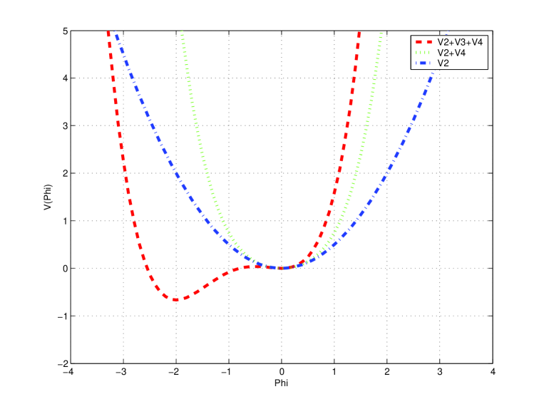
Figure 2: The potential $V$ of the scalar field $\phi$ in the case $\mu^{2}=1$, $\kappa=2.5$ and $\lambda=1$. In this case there are 3 extrema at $\phi^{(3)}=0$ with $V(\phi^{(3)}_{0})=0$; $\phi^{(2)}=-1/2$ with $V(\phi^{(3)}_{0})\approx 0.0365$ (local maximum) and $\phi^{(1)}=-2$ with $V(\phi^{(3)}_{0})=-0.6$ (the only real minimum).

In general, any minimum of the potential can be obtained for $\langle 0|\phi|0\rangle\equiv\phi_{0}$ which solves a minimum (extremum) condition

$$\partial V/\partial\phi=\phi(\mu^{2}+\kappa\phi+\lambda\phi^{2})=0.$$ (136)

There are 3 solutions. One is obviously $\phi^{(3)}_{0}=0$, which gives $V(\phi^{(3)}_{0})=0$. In principle, the two other solutions can be those of the quadratic equation $\lambda\phi^{2}+\kappa\phi+\mu^{2}=0$ (if $\kappa^{2}-4\lambda\mu^{2}>0$)

$$\phi^{(1,2)}_{0}=\frac{-\kappa\pm\sqrt{\kappa^{2}-4\lambda\mu^{2}}}{2\lambda}.$$

It is obvious that (if $\kappa^{2}-4\lambda\mu^{2}>0$) $|\phi^{(1)}_{0}|\neq|\phi^{(2)}_{0}|$ and in general $V(\phi^{(1)}_{0})\neq V(\phi^{(2)}_{0})$. Therefore, only one real minimum for the potential $V$ exists (see Fig. 2). It is important to note that there are no any solutions $\phi^{(1,2)}_{0}~{}$ if $~{}\kappa^{2}-4\lambda\mu^{2}<0~{}$ and the true minimum stays at $\phi^{(3)}_{0}=0$.

To simplify the problem, let us assume a “massless” scalar field $\phi$ with $\mu^{2}=0$. In this case, due to $\displaystyle\phi^{(1,2)}_{0}=\frac{-\kappa\pm\sqrt{\kappa^{2}}}{2\lambda}$ one has only one nonzero $\phi_{0}$, say

$$\phi^{(1)}_{0}=\frac{-\kappa}{\lambda}\equiv v,\quad{\rm and}\quad\phi^{(3)}_{0}=\phi^{(2)}_{0}=0.$$ (137)

Here the only quantity $v\equiv\langle\,0|\phi|0\,\rangle$ can be (as before) called the vacuum expectation value (vev) of the scalar field $\phi$ and has a sign opposite to $\kappa$. Lagrangian (135) no longer describes a particle with mass $\mu$ (or ever a massless particle when $\mu^{2}=0$). To interpret correctly the theory, one must expand around the real minimum $v$ by defining the field $\sigma$ as $\phi=v+\sigma$ and assuming that $\langle\,0|\sigma|0\,\rangle=0$. In terms of the new field $\sigma$, the potential $V(\phi)$ of (135) becomes ($\mu^{2}=0$ is assumed and $\kappa=-v\lambda$ is used)

$$V(\phi) = V(\sigma)=\frac{\kappa}{3}\phi^{3}+\frac{\lambda}{4}\phi^{4}=\left(\frac{\kappa}{3}+\frac{\lambda}{4}\phi\right)\phi^{3}=\left(-\frac{\lambda}{3}v+\frac{\lambda}{4}v+\frac{\lambda}{4}\sigma\right)(v+\sigma)^{3}=$$

$$= \frac{\lambda}{4}\left(\sigma-\frac{v}{3}\right)(v+\sigma)^{3}=\frac{\lambda}{4}\left(\sigma-\frac{v}{3}\right)(v^{3}+\sigma^{3}+3v^{2}\sigma+3v\sigma^{2})=$$

$$= \frac{\lambda}{4}\left(\sigma(v^{3}+\sigma^{3}+3v^{2}\sigma+3v\sigma^{2})-\frac{v}{3}(v^{3}+\sigma^{3}+3v^{2}\sigma+3v\sigma^{2})\right)=$$

$$= \frac{\lambda}{4}\left(v^{3}\sigma+\sigma^{4}+3v^{2}\sigma^{2}+3v\sigma^{3}-\frac{v^{4}}{3}-\frac{v}{3}\sigma^{3}-v^{3}\sigma-v^{2}\sigma^{2}\right)=$$

$$= \frac{\lambda}{4}\left(-\frac{v^{4}}{3}+\sigma^{4}+(v^{3}\sigma-v^{3}\sigma)+(3v^{2}\sigma^{2}-v^{2}\sigma^{2})+(3-\frac{1}{3})v\sigma^{3}\right)=$$

$$= \frac{\lambda}{4}\left(-\frac{v^{4}}{3}+\sigma^{4}+2v^{2}\sigma^{2}+\frac{8}{3}v\sigma^{3}\right)=\frac{\lambda v^{2}}{2}\sigma^{2}+\frac{2\lambda v}{3}\sigma^{3}+\frac{\lambda}{4}\sigma^{4}-\frac{\lambda v^{4}}{12}.$$

Finally, in terms of $\sigma$ the Lagrangian (135) becomes

$${\cal L} = \frac{1}{2}\partial_{\mu}\sigma\,\partial^{\mu}\sigma-V(\sigma)=\frac{1}{2}\partial_{\mu}\sigma\,\partial^{\mu}\sigma-\frac{\lambda v^{2}}{2}\sigma^{2}-\frac{2\lambda v}{3}\sigma^{3}-\frac{\lambda}{4}\sigma^{4}+\frac{\lambda v^{4}}{12}.$$

This is the theory of a scalar field of mass $m^{2}=\lambda v^{2}=-v\kappa>0$, with $\sigma^{3}$ and $\sigma^{4}$ being self-interactions. Note here $m^{2}=\lambda v^{2}=\frac{1}{2}m_{\kappa=0}^{2}$ (standard Higgs mechanism). This is, perhaps, due to our assumption $\mu^{2}=0$. Since the cubic terms in the initial Lagrangian, no any reflexion symmetry was broken. Therefore, one obtains a nonzero vev for the initial massless scalar field $\phi$, one got a mass for the new scalar field $\sigma$ without any spontaneously broken symmetry.

Now one should prove that the $\sigma$ cubic term does not spoil the zero-vev status of the $\sigma$ field. On this way one could obtain constraints on the term $-\frac{2\lambda v}{3}\sigma^{3}$.

Indeed, now again one has a $\sigma^{3}$ term in the potential

$$V(\sigma)=\frac{\lambda v^{2}}{2}\sigma^{2}+\frac{2\lambda v}{3}\sigma^{3}+\frac{\lambda}{4}\sigma^{4}-\frac{\lambda v^{4}}{12}=\frac{\lambda}{4}\left(2v^{2}\sigma^{2}+\frac{8}{3}v\sigma^{3}+\sigma^{4}-\frac{v^{4}}{3}\right).$$

The goal is to avoid any minimum at $\sigma\neq 0$. Applying now the extremum condition (136) to this potential one can obtain it in the form

$$\frac{\partial V}{\partial\sigma}=\lambda v^{2}\sigma+2\lambda v\sigma^{2}+\lambda\sigma^{3}=\lambda\sigma(\sigma^{2}+2v\sigma+v^{2})=\lambda\sigma(\sigma+v)^{2}=0.$$ (138)

There are two solutions of the equation: $\sigma=0$ and $\sigma=-v$. Substituting both into the potential above one finds

$$V(\sigma=0)=-\frac{\lambda v^{4}}{12}<0\qquad{\rm and}\qquad V(\sigma=-v)=0.$$

Therefore, always a true minimum is at $\sigma=0$.

Finally, it looks like that in the SM with the complex SU(2) doublet of scalar fields $\Phi$ given by eq. (29) it is also possible to use the “$\phi^{3}$” term if the Higgs potential (30) is taken, say, in the form

$$V(\Phi)={\mu^{2}}\,|\Phi|^{2}+\frac{2\sqrt{2}}{3}\kappa\,|\Phi|^{3}+{\lambda}\,|\Phi|^{4},\qquad{\rm where}\qquad|\Phi|=\sqrt{\Phi^{\dagger}\Phi}.$$

VI.3 Some relations

Consider in detail transformaton of the Abelian Largangian from section II.3, eq. (II.3)

$${\cal L} = -\frac{1}{4}F_{\mu\nu}F^{\mu\nu}+(\partial_{\mu}+ieA_{\mu})\phi^{*}(\partial^{\mu}-ieA^{\mu})\phi-V(\phi)$$ (139)

$${\rm with} ~{}V(\phi)~{}=~{}\mu^{2}\phi^{*}\phi+\lambda(\phi^{*}\phi)^{2}$$ (140)

after substitution in it of the complex scalar field in the form

$$\phi(x)=\frac{1}{\sqrt{2}}\left(v+\eta(x)+i\xi(x)\right)\equiv\frac{1}{\sqrt{2}}(v+\phi_{1}+i\phi_{2}).$$

The product of the covariant derivatives from (139) becomes

$$(D_{\mu}\phi)^{*}(D^{\mu}\phi) \equiv (\partial_{\mu}+ieA_{\mu})\phi^{*}\,(\partial^{\mu}-ieA^{\mu})\phi=(\partial_{\mu}\phi^{*}+ieA_{\mu}\phi^{*})\,(\partial^{\mu}\phi-ieA^{\mu}\phi)$$ (141)

$$= (\partial_{\mu}\phi)^{*}(\partial^{\mu}\phi)-ie(\partial_{\mu}\phi)^{*}A^{\mu}\phi+ie(\partial^{\mu}\phi)A_{\mu}\phi^{*}+e^{2}A_{\mu}A^{\mu}\,\phi^{*}\phi.$$

Furthermore

$$(\partial_{\mu}\phi)^{*} = \left({\partial_{\mu}\frac{1}{\sqrt{2}}\left(v+\eta+i\xi\right)}\right)^{*}=\frac{1}{\sqrt{2}}\left(\partial_{\mu}\eta-i\partial_{\mu}\xi\right),$$

$$(\partial^{\mu}\phi) = \left({\partial^{\mu}\frac{1}{\sqrt{2}}\left(v+\eta+i\xi\right)}\right)=\frac{1}{\sqrt{2}}\left(\partial^{\mu}\eta+i\partial^{\mu}\xi\right),$$

$$(\partial_{\mu}\phi)^{*}(\partial^{\mu}\phi) = \frac{1}{2}\left(\partial_{\mu}\eta\ \partial^{\mu}\eta+i\partial_{\mu}\eta\ \partial^{\mu}\xi-i\partial_{\mu}\xi\ \partial^{\mu}\eta+\partial_{\mu}\xi\ \partial^{\mu}\xi\right)=\frac{1}{2}\partial_{\mu}\eta\ \partial^{\mu}\eta+\frac{1}{2}\partial_{\mu}\xi\ \partial^{\mu}\xi,$$

$$(\partial_{\mu}\phi)^{*}\phi = \frac{1}{{2}}\left(\partial_{\mu}\eta-i\partial_{\mu}\xi\right)\left(v+\eta+i\xi\right)=\frac{v}{{2}}\left(\partial_{\mu}\eta-i\partial_{\mu}\xi\right)+\frac{1}{{2}}\left(\partial_{\mu}\eta-i\partial_{\mu}\xi\right)\left(\eta+i\xi\right)=$$

$$= \frac{v}{{2}}\left(\partial_{\mu}\eta-i\partial_{\mu}\xi\right)+\frac{1}{{2}}\left(\eta\partial_{\mu}\eta+i\xi\partial_{\mu}\eta-i\eta\partial_{\mu}\xi+\xi\partial_{\mu}\xi\right),$$

$$(\partial^{\mu}\phi)\phi^{*} = \frac{1}{{2}}\left(\partial^{\mu}\eta+i\partial^{\mu}\xi\right)\left(v+\eta-i\xi\right)=\frac{v}{{2}}\left(\partial^{\mu}\eta+i\partial^{\mu}\xi\right)+\frac{1}{{2}}\left(\partial^{\mu}\eta+i\partial^{\mu}\xi\right)(\eta-i\xi)=$$

$$= \frac{v}{{2}}\left(\partial^{\mu}\eta+i\partial^{\mu}\xi\right)+\frac{1}{{2}}\left(\eta\partial^{\mu}\eta-i\xi\partial^{\mu}\eta+i\eta\partial^{\mu}\xi+\xi\partial^{\mu}\xi\right),$$

$$\phi^{*}\phi = \frac{1}{2}\left(v+\eta-i\xi\right)\left(v+\eta+i\xi\right)=\frac{1}{2}\left((v+\eta)^{2}+\xi^{2}\right)=\frac{1}{2}\left(v^{2}+2v\eta+\eta^{2}+\xi^{2}\right),$$

$$(\phi^{*}\phi)^{2} = \frac{1}{4}\left(v^{2}+2v\eta+\eta^{2}+\xi^{2}\right)\left(v^{2}+2v\eta+\eta^{2}+\xi^{2}\right)=$$

$$= \frac{v^{2}}{4}\left(v^{2}+2v\eta+\eta^{2}+\xi^{2}\right)+\frac{v\eta}{2}\left(v^{2}+2v\eta+\eta^{2}+\xi^{2}\right)$$

$$+ \frac{\eta^{2}}{4}\left(v^{2}+2v\eta+\eta^{2}+\xi^{2}\right)+\frac{\xi^{2}}{4}\left(v^{2}+2v\eta+\eta^{2}+\xi^{2}\right)$$

$$= \frac{1}{4}\left(v^{4}+2v^{3}\eta+v^{2}\eta^{2}+v^{2}\xi^{2}+2v^{3}\eta+4v^{2}\eta^{2}+2v\eta^{3}+2v\eta\xi^{2}\right.$$

$$+ \left.v^{2}\eta^{2}+2v\eta^{3}+\eta^{4}+\xi^{2}\eta^{2}+v^{2}\xi^{2}+2v\eta\xi^{2}+\eta^{2}\xi^{2}+\xi^{4}\right)$$

$$= \frac{1}{4}\left(v^{4}+\eta^{4}+\xi^{4}+4v^{3}\eta+6v^{2}\eta^{2}+2v^{2}\xi^{2}+4v\eta^{3}+4v\eta\xi^{2}+2\eta^{2}\xi^{2}\right).$$

Substituting these expansions in the derivative product (141) and the potential (140) one obtians

$$(D_{\mu}\phi)^{*}(D^{\mu}\phi) = (\partial_{\mu}\phi)^{*}(\partial^{\mu}\phi)+e^{2}A_{\mu}A^{\mu}\,\phi^{*}\phi-ieA^{\mu}(\partial_{\mu}\phi)^{*}\phi+ieA_{\mu}(\partial^{\mu}\phi)\phi^{*}=$$

$$= \frac{1}{2}\partial_{\mu}\eta\ \partial^{\mu}\eta+\frac{1}{2}\partial_{\mu}\xi\ \partial^{\mu}\xi+\frac{e^{2}}{2}A_{\mu}A^{\mu}(v^{2}+2v\eta+\eta^{2}+\xi^{2})$$

$$-\frac{iev}{2}A^{\mu}(\partial_{\mu}\eta-i\partial_{\mu}\xi)-\frac{ie}{2}A^{\mu}(\eta\partial_{\mu}\eta+i\xi\partial_{\mu}\eta-i\eta\partial_{\mu}\xi+\xi\partial_{\mu}\xi)$$

$$+\frac{iev}{2}A_{\mu}(\partial^{\mu}\eta+i\partial^{\mu}\xi)+\frac{ie}{{2}}A_{\mu}(\eta\partial^{\mu}\eta-i\xi\partial^{\mu}\eta+i\eta\partial^{\mu}\xi+\xi\partial^{\mu}\xi)=$$

$$= \frac{1}{2}\partial_{\mu}\eta\ \partial^{\mu}\eta+\frac{1}{2}\partial_{\mu}\xi\ \partial^{\mu}\xi+\frac{e^{2}v^{2}}{2}A_{\mu}A^{\mu}+\frac{e^{2}}{2}A_{\mu}A^{\mu}(2v\eta+\eta^{2}+\xi^{2})-{ev}A^{\mu}\partial_{\mu}\xi$$

$$-\frac{ie}{2}\left(A^{\mu}(\eta\partial_{\mu}\eta+i\xi\partial_{\mu}\eta-i\eta\partial_{\mu}\xi+\xi\partial_{\mu}\xi)-A_{\mu}(\eta\partial^{\mu}\eta-i\xi\partial^{\mu}\eta+i\eta\partial^{\mu}\xi+\xi\partial^{\mu}\xi)\right)$$

$$(D_{\mu}\phi)^{*}(D^{\mu}\phi) = \frac{1}{2}\partial_{\mu}\eta\ \partial^{\mu}\eta+\frac{1}{2}\partial_{\mu}\xi\ \partial^{\mu}\xi+\frac{e^{2}v^{2}}{2}A_{\mu}A^{\mu}+\frac{e^{2}}{2}A_{\mu}A^{\mu}(2v\eta+\eta^{2}+\xi^{2})-{ev}A^{\mu}\partial_{\mu}\xi$$

$$+ eA^{\mu}\xi\partial_{\mu}\eta-eA^{\mu}\eta\partial_{\mu}\xi.$$

$$V(\phi) = \mu^{2}\phi^{*}\phi+\lambda(\phi^{*}\phi)^{2}=\frac{\mu^{2}}{2}\left(v^{2}+2v\eta+\eta^{2}+\xi^{2}\right)$$

$$+ \frac{\lambda}{4}\left(v^{4}+\eta^{4}+\xi^{4}+4v^{3}\eta+6v^{2}\eta^{2}+2v^{2}\xi^{2}+4v\eta^{3}+4v\eta\xi^{2}+2\eta^{2}\xi^{2}\right).$$

With the minimun realtion $\mu^{2}=-v^{2}\lambda$ the potential becomes

$$V(\phi) = -\frac{v^{2}\lambda}{2}\left(v^{2}+2v\eta+\eta^{2}+\xi^{2}\right)$$

$$+ \frac{\lambda}{4}\left(v^{4}+\eta^{4}+\xi^{4}+4v^{3}\eta+6v^{2}\eta^{2}+2v^{2}\xi^{2}+4v\eta^{3}+4v\eta\xi^{2}+2\eta^{2}\xi^{2}\right)=$$

$$= -\frac{v^{4}\lambda}{2}-{v^{3}\lambda}\eta-\frac{v^{2}\lambda}{2}\eta^{2}-\frac{v^{2}\lambda}{2}\xi^{2}$$

$$+\frac{v^{4}\lambda}{4}+\frac{\lambda}{4}\eta^{4}+\frac{\lambda}{4}\xi^{4}+{v^{3}\lambda}\eta+\frac{3v^{2}\lambda}{2}\eta^{2}+\frac{v^{2}\lambda}{2}\xi^{2}+{v\lambda}\eta^{3}+{v\lambda}\eta\xi^{2}+\frac{\lambda}{2}\eta^{2}\xi^{2}$$

$$V(\phi) = -\frac{v^{4}\lambda}{4}+{v^{2}\lambda}\eta^{2}+\frac{\lambda}{4}\eta^{4}+\frac{\lambda}{4}\xi^{4}+{v\lambda}\eta^{3}+{v\lambda}\eta\xi^{2}+\frac{\lambda}{2}\eta^{2}\xi^{2}.$$

Collecting now all terms together one can obtain the Abelian Lagrangian (139) in the form

$${\cal L} = -\frac{1}{4}F_{\mu\nu}F^{\mu\nu}+(D_{\mu}\phi)^{*}(D^{\mu}\phi)-V(\phi)=$$

$$= -\frac{1}{4}F_{\mu\nu}F^{\mu\nu}+\frac{1}{2}\partial_{\mu}\eta\,\partial^{\mu}\eta+\frac{1}{2}\partial_{\mu}\xi\,\partial^{\mu}\xi$$

$$+\frac{e^{2}v^{2}}{2}A_{\mu}A^{\mu}+\frac{e^{2}}{2}A_{\mu}A^{\mu}(2v\eta+\eta^{2}+\xi^{2})-{ev}A^{\mu}\partial_{\mu}\xi+eA^{\mu}\xi\partial_{\mu}\eta-eA^{\mu}\eta\partial_{\mu}\xi$$

$$-{v^{2}\lambda}\eta^{2}-\frac{\lambda}{4}(\eta^{2}+\xi^{2})^{2}-{v\lambda}\eta(\eta^{2}+\xi^{2})+\frac{v^{4}\lambda}{4}.$$

With $\eta=\phi_{1}$ and $\xi=\phi_{2}$ the relevant Lagrangian from Gaillard:1977wu is

$${\cal L} \equiv -\frac{1}{4}F_{\mu\nu}F^{\mu\nu}+(\partial^{\mu}+ieA^{\mu})\phi^{*}(\partial_{\mu}-ieA_{\mu})\phi-\mu^{2}\phi^{*}\phi-\lambda(\phi^{*}\phi)^{2}=$$

$$= -\frac{1}{4}F_{\mu\nu}F^{\mu\nu}+\frac{1}{2}(\partial_{\mu}\phi_{1})^{2}+\frac{1}{2}(\partial_{\mu}\phi_{2})^{2}-\phi_{1}(\mu^{2}+\lambda v^{2})-\frac{1}{2}\phi_{2}^{2}(\mu^{2}+v^{2}\lambda)$$

$$+\frac{e^{2}v^{2}}{2}A_{\mu}A^{\mu}+\frac{e^{2}}{2}A_{\mu}A^{\mu}(\phi_{1}^{2}+\phi_{2}^{2})+e^{2}vA_{\mu}A^{\mu}\phi_{1}-evA_{\mu}\partial^{\mu}\phi_{2}+eA_{\mu}(\partial^{\mu}\phi_{1})\phi_{2}-eA_{\mu}(\partial^{\mu}\phi_{2})\phi_{1}$$

$$-\frac{1}{2}\phi_{1}^{2}(\mu^{2}+3v^{2}\lambda)-\frac{\lambda}{4}(\phi_{1}^{2}+\phi_{2}^{2})^{2}-\lambda v\phi_{1}(\phi_{1}^{2}+\phi_{2}^{2})+\frac{v^{4}\lambda}{4}.$$

In the unitary gauge (22) Lagrangian (15) or (VI.3) with $\mu^{2}=-v^{2}\lambda$ transforms as follows:

$${\cal L} = \frac{1}{2}(\partial_{\mu}+ieA_{\mu})(v+\eta)(\partial^{\mu}-ieA^{\mu})(v+\eta)-\frac{\mu^{2}}{2}(v+\eta)^{2}-\frac{\lambda}{4}(v+\eta)^{4}-\frac{F_{\mu\nu}F^{\mu\nu}}{4}=$$

$$= \frac{1}{2}(\partial_{\mu}\eta+ieA_{\mu}(v+\eta))(\partial^{\mu}\eta-ieA^{\mu}(v+\eta))-\frac{F_{\mu\nu}F^{\mu\nu}}{4}$$

$$-\frac{v^{2}\lambda}{2}(-v^{2}-2v\eta-\eta^{2})-\frac{\lambda}{4}(v^{4}+4v^{3}\eta+6v^{2}\eta^{2}+4v\eta^{3}+\eta^{4})=$$

$$= \frac{1}{2}(\partial_{\mu}\eta\partial^{\mu}\eta-ie\partial_{\mu}\eta A^{\mu}(v+\eta)+ieA_{\mu}\partial^{\mu}\eta(v+\eta))+\frac{1}{2}e^{2}A_{\mu}A^{\mu}(v^{2}+2v\eta+\eta^{2})$$

$$-\frac{F_{\mu\nu}F^{\mu\nu}}{4}-\frac{\lambda}{4}(-2v^{4}-4v^{3}\eta-2v^{2}\eta^{2}+v^{4}+4v^{3}\eta+6v^{2}\eta^{2}+4v\eta^{3}+\eta^{4})\to$$

$${\cal L} = \frac{1}{2}\partial_{\mu}\eta\partial^{\mu}\eta-\frac{2v^{2}\lambda}{2}\eta^{2}-\frac{F_{\mu\nu}F^{\mu\nu}}{4}+\frac{e^{2}v^{2}}{2}A_{\mu}A^{\mu}+\frac{e^{2}}{2}A_{\mu}A^{\mu}(2v\eta+\eta^{2})+\frac{v^{4}\lambda}{4}-{\lambda}v\eta^{3}-\frac{\lambda}{4}\eta^{4}.$$

If one ignores the vector field $V_{\mu}$ (consider the pure complex scalar field, see section II.2 and (9)) and introduces the Higgs mass $m_{H}=\sqrt{2\lambda v^{2}}\equiv\sqrt{2}|\mu|$ the Lagrangian takes the form

$${\cal L} = \frac{1}{2}\partial_{\mu}\eta\,\partial^{\mu}\eta+\frac{1}{2}\partial_{\mu}\xi\,\partial^{\mu}\xi-\frac{\lambda}{4}\eta^{4}-\frac{\lambda}{4}\xi^{4}-\frac{\lambda}{2}\eta^{2}\xi^{2}+\frac{v^{4}\lambda}{4}-\frac{m^{2}_{H}}{2}\eta^{2}-v\lambda\eta^{3}-v\lambda\eta\xi^{2}.$$

Consider transformation of the product of the covariant derivatives $|D_{\mu}\Phi|^{2}$ (II.4) in the Standard Model (see section II.4). First, one has to insert the explicit forms of Pauli matrices (114) into $D_{\mu}\Phi$ and then contract $(D_{\mu}\Phi)^{\dagger}$ and $|D_{\mu}\Phi|^{2}$:

$$D_{\mu}\Phi = \left(\partial_{\mu}-ig_{2}\frac{\tau_{a}}{2}W_{\mu}^{a}-ig_{1}\frac{Y_{H}}{2}B_{\mu}\right)\Phi=$$

$$= \left(\left(\begin{array}[]{cc}1&0\\ 0&1\end{array}\right)\left(\partial_{\mu}-\frac{ig_{1}Y_{H}}{2}B_{\mu}\right)-\frac{ig_{2}}{2}\left(\left(\begin{array}[]{cc}0&1\\ 1&0\end{array}\right)W_{\mu}^{1}+\left(\begin{array}[]{cc}0&-i\\ i&0\end{array}\right)W_{\mu}^{2}+\left(\begin{array}[]{cc}1&0\\ 0&-1\end{array}\right)W_{\mu}^{3}\right)\right)\Phi$$

$$= \left(\begin{array}[]{cc}\partial_{\mu}-\frac{i}{2}\left({g_{2}}W_{\mu}^{3}+{g_{1}Y_{H}}B_{\mu}\right)&-\frac{ig_{2}}{2}(W_{\mu}^{1}-iW_{\mu}^{2})\\ -\frac{ig_{2}}{2}(W_{\mu}^{1}+iW_{\mu}^{2})&\partial_{\mu}+\frac{i}{2}\left({g_{2}}W_{\mu}^{3}-{g_{1}Y_{H}}B_{\mu}\right)\end{array}\right)\frac{1}{\sqrt{2}}\left(\begin{array}[]{c}0\\ v+h(x)\end{array}\right)=$$

$$= \frac{1}{\sqrt{2}}\left(\begin{array}[]{c}-\frac{ig_{2}}{2}(W_{\mu}^{1}-iW_{\mu}^{2})(v+h(x))\\ \partial_{\mu}h(x)+\frac{i}{2}\left({g_{2}}W_{\mu}^{3}-{g_{1}Y_{H}}B_{\mu}\right)(v+h(x))\end{array}\right);$$

$$(D^{\mu}\Phi)^{\dagger} = \Phi^{\dagger}\left(\partial^{\mu}-ig_{2}\frac{\tau_{a}}{2}W^{\mu}_{a}-ig_{1}\frac{Y_{H}}{2}B^{\mu}\right)^{\dagger}=\frac{1}{\sqrt{2}}\left(\begin{array}[]{c}-\frac{ig_{2}}{2}(W^{\mu}_{1}-iW^{\mu}_{2})(v+h(x))\\ \partial^{\mu}h(x)+\frac{i}{2}\left({g_{2}}W^{\mu}_{3}-{g_{1}Y_{H}}B^{\mu}\right)(v+h(x))\end{array}\right)^{\dagger}$$

$$= \frac{1}{\sqrt{2}}\left(\frac{ig_{2}}{2}(W_{\mu}^{1}+iW_{\mu}^{2})(v+h(x)),\ \partial_{\mu}h(x)-\frac{i}{2}\left({g_{2}}W_{\mu}^{3}-{g_{1}Y_{H}}B_{\mu}\right)(v+h(x))\right);$$

$$|D_{\mu}\Phi|^{2} \equiv (D^{\mu}\Phi)^{\dagger}(D_{\mu}\Phi)=\left|\left(\partial_{\mu}-ig_{2}\frac{\tau_{a}}{2}W_{\mu}^{a}-ig_{1}\frac{Y_{H}}{2}B_{\mu}\right)\Phi\right|^{2}=$$

$$= \Phi^{\dagger}\left(\partial^{\mu}-ig_{2}\frac{\tau_{a}}{2}W^{\mu}_{a}-ig_{1}\frac{Y_{H}}{2}B^{\mu}\right)^{\dagger}\left(\partial_{\mu}-ig_{2}\frac{\tau_{a}}{2}W_{\mu}^{a}-ig_{1}\frac{Y_{H}}{2}B_{\mu}\right)\Phi=$$

$$= \frac{1}{2}\left|\left(\begin{array}[]{cc}\partial_{\mu}-\frac{i}{2}(g_{2}W_{\mu}^{3}+g_{1}Y_{H}B_{\mu})&-\frac{ig_{2}}{2}(W_{\mu}^{1}-iW^{2}_{\mu})\\ -\frac{ig_{2}}{2}(W_{\mu}^{1}+iW^{2}_{\mu})&\partial_{\mu}+\frac{i}{2}(g_{2}W_{\mu}^{3}-g_{1}Y_{H}B_{\mu})\end{array}\right)\left(\begin{array}[]{c}0\\ v+h(x)\end{array}\right)\right|^{2}$$

$$= \frac{1}{\sqrt{2}}\left(\frac{ig_{2}}{2}(W^{\mu}_{1}+iW^{\mu}_{2})(v+h),\ \partial^{\mu}h(x)-\frac{i}{2}\left({g_{2}}W^{\mu}_{3}-{g_{1}Y_{H}}B^{\mu}\right)(v+h)\right)$$

$$\times\frac{1}{\sqrt{2}}\left(\begin{array}[]{c}-\frac{ig_{2}}{2}(W_{\mu}^{1}-iW_{\mu}^{2})(v+h)\\ \partial_{\mu}h(x)+\frac{i}{2}\left({g_{2}}W_{\mu}^{3}-{g_{1}Y_{H}}B_{\mu}\right)(v+h)\end{array}\right)=$$

$$= \frac{1}{2}\left(-\frac{ig_{2}}{2}(W^{\mu}_{1}+iW^{\mu}_{2})(v+h)\frac{ig_{2}}{2}(W_{\mu}^{1}-iW_{\mu}^{2})(v+h)\right.$$

$$+ \left.\left(\partial^{\mu}h-\frac{i}{2}({g_{2}}W^{\mu}_{3}-{g_{1}Y_{H}}B^{\mu})(v+h)\right)\left(\partial_{\mu}h+\frac{i}{2}({g_{2}}W_{\mu}^{3}-{g_{1}Y_{H}}B_{\mu})(v+h)\right)\right)=$$

$$= \frac{g^{2}_{2}}{8}(v+h)^{2}(W^{\mu}_{1}+iW^{\mu}_{2})(W_{\mu}^{1}-iW_{\mu}^{2})+\frac{1}{2}\partial^{\mu}h(x)\partial_{\mu}h(x)+\frac{1}{8}(v+h)^{2}\left({g_{2}}W^{\mu}_{3}-{g_{1}Y_{H}}B^{\mu}\right)^{2},$$

$$|D_{\mu}\Phi|^{2} = \frac{1}{2}(\partial_{\mu}h)^{2}+\frac{g_{2}^{2}}{8}(v+h)^{2}|W_{\mu}^{1}+iW_{\mu}^{2}|^{2}+\frac{1}{8}(v+h)^{2}(g_{2}W_{\mu}^{3}-g_{1}Y_{H}B_{\mu})^{2}.$$

References

• (1) Haber H. E. // hep-ph/0409008.
• (2) Gunion J. F., Haber H. E., Kane G. L., and Dawson S. // The Higgs Hunter’s Guide. Perseus Publishing, Cambridge, MA 2000.
• (3) Gunion J. F., Haber H. E., Kane G. L., and Dawson S. // hep-ph/9302272.
• (4) Djouadi A. // hep-ph/0503172.
• (5) Glashow S. L. // Nucl. Phys. 1961. V.22. P.579–588.
• (6) Weinberg S. // Phys. Rev. Lett. 1967. V.19. P.1264–1266.
• (7) Salam A. // The standard model. Almqvist and Wiksells, Stockholm 1969. In *Elementary Particle Theory*, ed. N. Svartholm, p. 367.
• (8) Gell-Mann M. // Phys. Lett. 1964. V.8. P.214–215.
• (9) Fritzsch H., Gell-Mann M., and Leutwyler H. // Phys. Lett. 1973. V.B47. P.365–368.
• (10) Gross D. J. and Wilczek F. // Phys. Rev. Lett. 1973. V.30. P.1343–1346.
• (11) Politzer H. D. // Phys. Rev. Lett. 1973. V.30. P.1346–1349.
• (12) Kazakov D. I. // Beyond the standard model. CERN, Geneve 1989. In *Egmond-aan-Zee 1989, Proceedings, CERN-JINR School of Physics* 129-181.
• (13) Gaillard M. K. and Nikolic M. // Weak interactions. IN2P3, Paris 1977. 374 pp.
• (14) Higgs P. W. // Phys. Rev. Lett. 1964. V.13. P.508–509.
• (15) Higgs P. W. // Phys. Rev. 1966. V.145. P.1156–1163.
• (16) Kibble T. W. B. // Phys. Rev. 1967. V.155. P.1554–1561.
• (17) Kane G. L. // Modern elementary particle physics. Redwood city, USA: Addison-Wesley 1987. 344 pp.
• (18) Goldstone J. // Nuovo Cim. 1961. V.19. P.154–164.
• (19) Goldstone J., Salam A., and Weinberg S. // Phys. Rev. 1962. V.127. P.965–970.
• (20) Yao W. M. and others // J. Phys. 2006. V.G33. P.1–1232.
• (21) Aitchison I. J. R. // Field theory and standard model. CERN, Geneve 2004. Prepared for European School on High-Energy Physics, Tsakhkadzor, Armenia, 24 Aug - 6 Sep 2003.
• (22) Grojean C. // New approaches to electroweak symmetry breaking. Elsevier, Amsterdam 2005. Les Houches Summer School on Theoretical Physics: Session 84: Particle Physics Beyond the Standard Model, Les Houches, France, 1-26 Aug 2005.
• (23) Callaway D. J. E. // Nucl. Phys. 1984. V.B233. P.189.
• (24) Callaway D. J. E. // Phys. Rept. 1988. V.167. P.241.
• (25) Dashen R. F. and Neuberger H. // Phys. Rev. Lett. 1983. V.50. P.1897.
• (26) Wu Y.-Y. // Phys. Rev. 1995. V.D51. P.5276–5284 hep-ph/9502379.
• (27) Choudhury S. R., Mamta , and Dutta S. // Pramana 1998. V.50. P.163–171 hep-ph/9512422.
• (28) Lee B. W., Quigg C., and Thacker H. B. // Phys. Rev. 1977. V.D16. P.1519.
• (29) Chanowitz M. S. and Gaillard M. K. // Nucl. Phys. 1985. V.B261. P.379.
• (30) Linde A. D. // Phys. Lett. 1977. V.B70. P.306.
• (31) Weinberg S. // Phys. Rev. Lett. 1976. V.36. P.294–296.
• (32) Coleman S. R. and Weinberg E. // Phys. Rev. 1973. V.D7. P.1888–1910.
• (33) Quiros M. // hep-ph/9703412.
• (34) Sher M. // Phys. Rept. 1989. V.179. P.273–418.
• (35) Casas J. A., Espinosa J. R., and Quiros M. // Phys. Lett. 1996. V.B382. P.374–382 hep-ph/9603227.
• (36) Martin S. P. // hep-ph/9709356.
• (37) Hambye T. and Riesselmann K. // hep-ph/9708416.
• (38) Kolda C. F. and Murayama H. // JHEP 2000. V.07. P.035 hep-ph/0003170.
• (39) Okun L. B. // Leptons and quarks. Nauka: Moscow 1990. 346 pp. (second edition).
• (40) Okun L. B. // Leptons and quarks. Amsterdam, Netherlands: North-holland 1982. 361 pp.
• (41) Schmaltz M. and Tucker-Smith D. // Ann. Rev. Nucl. Part. Sci. 2005. V.55. P.229–270 hep-ph/0502182.
• (42) Quiros M. // hep-ph/0302189.
• (43) Nomura Y. // JHEP 2003. V.11. P.050 hep-ph/0309189.
• (44) Simmons E. H., Chivukula R. S., He H. J., Kurachi M., and Tanabashi M. // AIP Conf. Proc. 2006. V.857. P.34–45 hep-ph/0606019.
• (45) Hill C. T. and Simmons E. H. // Phys. Rept. 2003. V.381. P.235–402 hep-ph/0203079.
• (46) Gunion J. F. and Haber H. E. // Phys. Rev. 2003. V.D67. P.075019 hep-ph/0207010.
• (47) Cheng H.-C. and Low I. // JHEP 2003. V.09. P.051 hep-ph/0308199.
• (48) Okun L. B. // Physics of elementary particles. Nauka: Moscow 1984. 223 pp.
• (49) Yang C.-N. and Mills R. L. // Phys. Rev. 1954. V.96. P.191–195.
• (50) Behrends R. E., Finkelstein R. J., and Sirlin A. // Phys. Rev. 1956. V.101. P.866–873.
• (51) Kinoshita T. and Sirlin A. // Phys. Rev. 1959. V.113. P.1652–1660.
• (52) Ritbergen van T. and Stuart R. G. // Phys. Rev. Lett. 1999. V.82. P.488–491 hep-ph/9808283.
• (53) Dawson S. // hep-ph/0303191.
• (54) Kuhn J. H. // hep-ph/9707321.
• (55) Gray N., Broadhurst D. J., Grafe W., and Schilcher K. // Z. Phys. 1990. V.C48. P.673–680.
• (56) Melnikov K. and Ritbergen T. v. // Phys. Lett. 2000. V.B482. P.99–108 hep-ph/9912391.
• (57) Chetyrkin K. G. and Steinhauser M. // Phys. Rev. Lett. 1999. V.83. P.4001–4004 hep-ph/9907509.
• (58) Chetyrkin K. G. and Steinhauser M. // Nucl. Phys. 2000. V.B573. P.617–651 hep-ph/9911434.
• (59) Gorishnii S. G., Kataev A. L., Larin S. A., and Surguladze L. R. // Phys. Rev. 1991. V.D43. P.1633–1640.
• (60) Gorishnii S. G., Kataev A. L., Larin S. A., and Surguladze L. R. // Mod. Phys. Lett. 1990. V.A5. P.2703–2712.
• (61) Chetyrkin K. G. // Phys. Lett. 1997. V.B404. P.161–165 hep-ph/9703278.
• (62) Vermaseren J. A. M., Larin S. A., and Ritbergen van T. // Phys. Lett. 1997. V.B405. P.327–333 hep-ph/9703284.
• (63) Chetyrkin K. G., Kuhn J. H., and Steinhauser M. // Comput. Phys. Commun. 2000. V.133. P.43–65 hep-ph/0004189.