1 Introduction

The phenomenology of the strong interactions at low energies, where the coupling constant of Quantum Chromodynamics (QCD) becomes large and renders perturbation theory useless, remains one of the major challenges of modern particle physics. Only two rigorous approaches to this part of the standard model are known: lattice QCD; and the effective field theory called chiral perturbation theory. Both also offer the only ways to provide a firmer foundation for nuclear physics, rooted in the standard model.

These lectures provide an introduction to chiral perturbation theory, organised as follows. In Sect. 2, we present a few fundamental ideas on effective field theories in general. Section 3 introduces the basic concept and construction of chiral Lagrangians; a first application is the determination of the ratios of light quark masses. In Sect. 4, chiral perturbation theory is extended to higher orders, in particular, the relation of the quark mass expansion of the pion mass to pion-pion scattering is discussed in some detail. Section 5 extends chiral perturbation theory to include nucleons; the complications in doing loop calculations are explained, and the quark mass expansion of the nucleon mass is discussed in relation to pion-nucleon scattering. A final outlook summarises some major omissions that could not be covered here.

Several useful pedagogical introductions and review articles on the subject have been consulted in the course of the preparation of these lectures, see in particular [1, 2, 3, 4, 5, 6, 7], many of them being much more comprehensive than the present article, which are therefore recommended for further reading.

2 Effective field theories

The large number of different areas in physics describe phenomena at very disparate scales of length, time, energy, or mass. It is a rather intuitive idea that, as long as one is only interested in a particular parameter range, scales much bigger or much smaller than the ones one is interested in should not influence the description of the system in question too strongly. Indeed, the two fundamental revolutions in physics in the early 20th century did not come about earlier because they involve scales far removed from our everyday experience: for velocities far smaller than the speed of light, $v\ll c$, relativity effects can safely be ignored; and for energies and time scales much larger than Planck’s constant, $E\times t\gg\hslash$, quantum effects are rarely relevant.

One striking feature in particle physics is the extremely wide range of observed particle masses. Even ignoring neutrinos, the masses of the fermions comprise nearly six orders of magnitude, ranging from the electron mass $m_{e}=0.511$ MeV to the top quark mass $m_{t}\approx 180$ GeV. On the other hand, we can very well calculate the properties of certain systems, say, the spectrum of the hydrogen atom, without having any precise knowledge of $m_{t}$ at all. In this sense, very heavy particles do not seem to have a significant influence on the description of the system.

These rather informal ideas are explored more systematically in effective field theories. Let us, as an example, consider a theory with a set of “light” degrees of freedom $l_{i}$ and heavy fields $H_{j}$, their respective masses well separated by a scale $\Lambda$,

$$m_{l_{i}}\ll\Lambda\lesssim M_{H_{j}}~{}.$$

For energies well below $\Lambda$, the heavy particles can be integrated out of the generating functional, leaving behind an effective Lagrangian for the light degrees of freedom only,

$$\mathcal{L}(l_{i},H_{j})\stackrel{{\scriptstyle E\ll\Lambda}}{{\longrightarrow}}\mathcal{L}_{\rm eff}(l_{i})=\mathcal{L}_{d\leq 4}+\sum_{d>4}\frac{1}{\Lambda^{d-4}}\sum_{i_{d}}g_{i_{d}}O_{i_{d}}~{},$$ (1)

i.e. the procedure potentially generates non-renormalisable operators of dimension larger than 4. In a so-called “decoupling” effective field theory, the effects of the heavy fields $H_{j}$ enter $\mathcal{L}_{\rm eff}(l_{i})$ either as renormalisation effects of the effective coupling constants, or as new, higher-dimensional operators suppressed by inverse powers of the heavy mass $M_{H_{j}}$.

We want to briefly illustrate such decoupling effective theories with a classic example: electrodynamics far below the electron mass.

2.1 An example: light-by-light scattering

In Quantum Electrodynamics (QED), the only available mass scale is the mass of the electron $m_{e}$. If we consider QED at energies far below this mass scale, $\omega\ll m_{e}$, we should be able to write down an effective Lagrangian that contains only photons as dynamical degrees of freedom,

$$\mathcal{L}_{\rm QED}[\psi,\bar{\psi},A_{\mu}]\to\mathcal{L}_{\rm eff}[A_{\mu}]~{}.$$

However, the electrons present in the full theory generate effective interactions for the photon fields, contributing e.g. to photon–photon scattering, see Fig. 1.

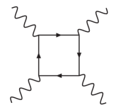
Figure 1: Feynman diagram for light-by-light scattering. 

However, we do not have to calculate the underlying loop diagrams explicitly in order to understand the structure of the effective theory; rather we can write it down directly in terms of the invariants $F_{\mu\nu}F^{\mu\nu}\propto\vec{E}^{2}-\vec{B}^{2}$, $F_{\mu\nu}\tilde{F}^{\mu\nu}\propto\vec{E}\cdot\vec{B}$. Considering only terms with up to four photon fields, we find

$$\mathcal{L}_{\rm eff}=\frac{1}{2}\bigl{(}\vec{E}^{2}-\vec{B}^{2}\bigr{)}+\frac{e^{4}}{16\pi^{2}m_{e}^{4}}\left[a\bigl{(}\vec{E}^{2}-\vec{B}^{2}\bigr{)}^{2}+b\bigl{(}\vec{E}\cdot\vec{B}\bigr{)}^{2}\right]+\ldots~{},$$ (2)

where the prefactor of the interaction term is taken from dimensional analysis, such that the coupling constants $a$ and $b$ are expected to be of order 1. These constants can only be calculated explicitly from the underlying theory, with the result $7a=b=14/45$ [8].

The following points are to be noted from this brief example, which are typical for the construction of (low-energy) effective field theories:

1. We have constructed the interaction terms in the Lagrangian based on the symmetries (gauge invariance, Lorentz invariance) of the underlying theory, which ought to be shared by the effective one.

2. We could only guess the order of magnitude of the effective coupling constants $a$, $b$ correctly, but their exact values are not determined by symmetry considerations alone; they have to be calculated explicitly from the dynamics of the fundamental theory.

3. By considering only the simplest invariant terms that can be constructed in terms of the field strength tensor $F_{\mu\nu}$ (and its adjoint) and no additional derivatives, we have implicitly performed a low-energy expansion of the amplitude, i.e. an expansion in powers of $(\omega/m_{e})^{2n}$.

4. It is obvious from (2) that the calculation of cross sections etc. is much simpler and more efficiently done using $\mathcal{L}_{\rm eff}$ than performing the calculation in full QED.

2.2 Weinberg’s conjecture

The following statement by Weinberg lies at the very heart of the successful application of effective field theories, using an effective Lagrangian framework:

Quantum Field Theory has no content besides unitarity, analyticity, cluster decomposition, and symmetries. [9]

This means that in order to calculate the S-matrix for any theory below some scale, simply use the most general effective Lagrangian consistent with these principles in terms of the appropriate asymptotic states. This is what we have done in the previous subsection for QED at very low energies; and we will now follow this principle in the construction of an effective theory for the strong interactions.

3 The strong interactions at low energies

3.1 The symmetries of Quantum Chromodynamics

The spectrum of states of strongly interacting particles displays some interesting features. Above a typical hadronic mass scale of about 1 GeV, there is a large number of states, both meson resonances and baryons. Only a very few (pseudoscalar) states, however, are significantly lighter than this mass scale: in particular the pions ($M_{\pi}\approx 140$ MeV), but also kaons ($M_{K}\approx 495$ MeV) and the eta ($M_{\eta}\approx 550$ MeV).

The widely accepted theory of the strong interactions is Quantum Chromodynamics, a theory formulated in terms of quark and gluon fields built on the principle of colour gauge invariance with the gauge group SU(3)_c. The running strong coupling constant leads to the phenomena of asymptotic freedom in the high-energy regime, but also to confinement of the quark and gluon degrees of freedom inside colour-neutral hadronic states. The large coupling prevents a use of perturbation theory at low energies, so there is no direct and obvious link between QCD and its fundamental degrees of freedom, and the relevant hadronic degrees of freedom as observed in the spectrum of mesons and baryons.

In order to construct a low-energy effective theory for the strong interactions, we have to investigate the symmetries of the QCD Lagrangian more closely. For this purpose, we decompose the quark fields into its chiral components according to

$$q=\frac{1}{2}(1-\gamma_{5})q+\frac{1}{2}(1+\gamma_{5})q=P_{L}q+P_{R}q~{}=~{}q_{L}+q_{R}~{}.$$ (3)

Using this, we can write the QCD Lagrangian as

$$\mathcal{L}_{\rm QCD} = \mathcal{L}_{\rm QCD}^{0}-\mathcal{L}_{\rm QCD}^{m}+\ldots~{},$$

$$\mathcal{L}_{\rm QCD}^{0} = -\frac{1}{2}{\rm Tr}\,G_{\mu\nu}^{a}G^{\mu\nu,a}+i\bar{q}_{L}\!\not\!\!Dq_{L}+i\bar{q}_{R}\!\not\!\!Dq_{R}~{},$$

$$\mathcal{L}_{\rm QCD}^{m} = \bar{q}_{L}\mathcal{M}q_{R}+\bar{q}_{R}\mathcal{M}^{\dagger}q_{L}~{},$$ (4)

where $D_{\mu}$ is the covariant derivative, $G_{\mu\nu}^{a}$ the gluon field strength tensor, $q$ collects the light quark flavours $q^{T}=(u,d,s)$, and $\mathcal{M}={\rm diag}(m_{u},\,m_{d},\,m_{s})$ is the quark mass matrix. The ellipse denotes the heavier quark flavours, gauge fixing terms etc. We note that, besides the obvious symmetries like Lorentz-invariance, ${\rm SU}(3)_{c}$ gauge invariance, and the discrete symmetries $P$, $C$, $T$, $\mathcal{L}_{\rm QCD}$ displays a chiral symmetry in the limit of vanishing quark masses (which is hence called “chiral limit”): $\mathcal{L}_{\rm QCD}^{0}$ is invariant under chiral $U(3)_{L}\times U(3)_{R}$ flavour transformations,

$$(q_{L},q_{R})\longmapsto(Lq_{L},Rq_{R})~{},\quad L,R\in{\rm U}(3)_{L,R}~{}.$$ (5)

As the masses of the three light quarks are small on the typical hadronic scale,

$$m_{u,d,s}\ll 1~{}{\rm GeV}\approx\Lambda_{hadr}~{},$$

there is hope that the real world is not too far from the chiral limit, such that one may invoke a perturbative expansion in the quark masses. The effective theory constructed in the following, based on this idea, is therefore called “chiral perturbation theory” (ChPT).

If we rewrite the symmetry group according to

$${\rm U}(3)_{L}\times{\rm U}(3)_{R}={\rm SU}(3)_{L}\times{\rm SU}(3)_{R}\times{\rm U}(1)_{V}\times{\rm U}(1)_{A}~{},$$ (6)

where we have introduced vector $V=L+R$ and axial vector $A=L-R$ transformations, and consider the Noether currents associated with this symmetry group, it turns out that the different parts of it are realised in very different ways in nature:

• The ${\rm U}(1)_{V}$ current $V^{\mu,0}=\bar{q}\gamma_{\mu}q$, the quark number or baryon number current, is a conserved current in the standard model.

• The ${\rm U}(1)_{A}$ current $A^{\mu,0}=\bar{q}\gamma_{\mu}\gamma_{5}q$ is broken by quantum effects, the ${\rm U}(1)_{A}$ anomaly, and is not a conserved current of the quantum theory.

As far as the chiral symmetry group ${\rm SU}(3)_{L}\times{\rm SU}(3)_{R}$ and its conserved currents

$$\begin{array}[]{rclrcl}V^{\mu,a}&=&\bar{q}\gamma^{\mu}\dfrac{\lambda^{a}}{2}q~{},&\quad\partial_{\mu}V^{\mu,a}&=&0~{},\\[5.69054pt] A^{\mu,a}&=&\bar{q}\gamma^{\mu}\gamma_{5}\dfrac{\lambda^{a}}{2}q~{},&\quad\partial_{\mu}A^{\mu,a}&=&0~{},\end{array}\quad a=1,\ldots,8$$

are concerned, they are certainly broken explicitly by the quark masses, but this is expected to be a small effect. Hence the main question is whether chiral symmetry is realised in nature in the Wigner–Weyl mode, i.e. the symmetry is manifest in the spectrum in terms of multiplets, or whether it is realised as the Goldstone mode, i.e. the symmetry is hidden or spontaneously broken.

Can chiral symmetry of the strong interactions be in the Wigner–Weyl mode? In this case, the conserved axial charges annihilating the vacuum,

$$Q^{a}_{5}|0\rangle=0~{},\quad Q_{5}^{a}=\int d^{3}xA^{0,a}(x)~{},$$

would lead to parity doubling in the hadron spectrum. Phenomenologically, we find (approximate) SU(3)_V multiplets, but no parity doubling is observed. Furthermore, unbroken chiral symmetry would lead to a vanishing difference of the vector–vector and axial–axial vacuum correlators, $\langle 0|VV|0\rangle-\langle 0|AA|0\rangle=0$. This difference can be measured in hadronic tau decays $\tau\to\nu_{\tau}+n\,\pi$, leading to a non-vanishing result [10].

If chiral symmetry is, however, realised in the Goldstone mode, the Vafa–Witten theorem [11] asserts that the vector subgroup should remain unbroken, in accordance with the observation of hadronic multiplets, so the symmetry breaking pattern would be

$${\rm SU}(3)_{L}\times{\rm SU}(3)_{R}\stackrel{{\scriptstyle{\rm SSB}}}{{\longrightarrow}}{\rm SU}(3)_{V}~{}.$$ (7)

The axial charges then commute with the Hamiltonian, but do not leave the ground state invariant. As a consequence, massless excitations, so-called “Goldstone bosons” appear, which are non-interacting for vanishing energy. In the case at hand, the 8 Goldstone bosons should be pseudoscalars, which the lightest hadrons in the spectrum indeed are, namely $\pi^{\pm}$, $\pi^{0}$, $K^{\pm}$, $K^{0}$, $\bar{K}^{0}$, and $\eta$. The task is now to construct a low-energy theory for these Goldstone bosons. This is an example for a non-decoupling effective field theory: in contrast to the example of QED at energies below the electron mass described earlier, the transition from the full to the effective theory proceeds via a phase transition / via spontaneous symmetry breakdown, in the course of which new light degrees of freedom are generated.

3.2 Construction of the effective Lagrangian

We want to develop a general formalism [12] to construct the effective theory for the Goldstone bosons corresponding to a symmetry group $G$ spontaneously broken to its subgroup $H$, hence $G\stackrel{{\scriptstyle\rm SSB}}{{\longrightarrow}}H$, where ${\rm dim}(G)-{\rm dim}(H)=n$. We combine the Goldstone boson fields in a vector $\vec{\phi}=(\phi_{1},\ldots,\phi_{n})$, $\phi_{i}:~{}M^{4}\to{\mathbb{R}}$ (where $M^{4}$ denotes Minkowski space). The symmetry group $G$ acts on $\vec{\phi}$ according to

$$g\in G\,:\quad\vec{\phi}\longmapsto\vec{\phi}^{\prime}=\vec{f}\bigl{(}g,\vec{\phi}\bigr{)}~{},$$

which has to obey the composition law

$$\vec{f}\bigl{(}g_{1},\vec{f}(g_{2},\vec{\phi})\bigr{)}=\vec{f}\bigl{(}g_{1}g_{2},\vec{\phi}\bigr{)}~{}.$$

Consider the image of the origin $\vec{f}(g,\vec{0})$: elements leaving the origin invariant form a subgroup, the conserved subgroup $H$. Now we have

$$\forall g\in G\quad\forall h\in H\quad\vec{f}(gh,\vec{0})=\vec{f}(g,\vec{0})~{},$$

therefore $\vec{f}$ maps the quotient space $G/H$ onto the space of Goldstone boson fields. This mapping is invertible, as $\vec{f}(g_{1},\vec{0})=\vec{f}(g_{2},\vec{0})$ implies $g_{1}g_{2}^{-1}\in H$. Hence we conclude that the Goldstone bosons can be identified with elements of $G/H$. For $q_{i}\in G/H$, the action of $G$ on $G/H$ is then given by

$$gq_{1}=q_{2}h(g,\,q_{1})~{},\quad h(g,\,q_{1})\in H~{},$$

therefore the coordinates of $G/H$ transform nonlinearly under $G$.

In the case of QCD, we denote the group elements by $g\sim(g_{R},\,g_{L})$, $g_{R/L}\in{\rm SU}(3)_{R/L}$, with the composition law

$$g_{1}g_{2}=(g_{R_{1}},\,g_{L_{1}})(g_{R_{2}},\,g_{L_{2}})=(g_{R_{1}}g_{R_{2}},\,g_{L_{1}}g_{L_{2}})~{}.$$

The choice of a representative element inside each equivalence class is in principle arbitrary, the convention for $gH\in G/H$ is to rewrite $(g_{R},\,g_{L})=(\mathbb{E},\,{g_{L}g_{R}^{-1}})(g_{R},\,g_{R})$ and to characterise each element of $G/H$, i.e. each Goldstone boson, uniquely by a unitary matrix

$$U=g_{L}g_{R}^{-1}=\exp\left(\frac{i\lambda_{a}{\phi_{a}}}{{F^{\prime}}}\right)~{}.$$ (8)

Here, the $\phi_{a}$, $a=1,\ldots,8$ are the Goldstone boson fields, and $F^{\prime}$ is a dimensionful constant to be determined later. How does $U$ transform under the chiral group? We find

$$(R,L)(\mathbb{E},U)\cdot H=(\mathbb{E},LUR^{\dagger})(R,R)\cdot H=(\mathbb{E},{LUR^{\dagger}})\cdot H~{},$$

therefore

$$U\stackrel{{\scriptstyle G}}{{\longmapsto}}LUR^{\dagger}~{}.$$ (9)

3.3 The leading-order Lagrangian

Now we know how the Goldstone boson fields transform under chiral transformations, we can proceed to construct a Lagrangian in terms of the matrix $U$ that is invariant under ${\rm SU}(3)_{L}\times{\rm SU}(3)_{R}$. As we want to construct a low-energy effective theory, the guiding principle is to use the power of momenta or derivatives to order the importance of various possible terms. “Low energies” here refer to a scale well below 1 GeV, i.e. an energy region where the Goldstone bosons are the only relevant degrees of freedom.

Lorentz invariance dictates that Lagrangian terms can only come in even powers of derivatives, hence $\mathcal{L}$ is of the form

$$\mathcal{L}=\mathcal{L}^{(0)}+\mathcal{L}^{(2)}+\mathcal{L}^{(4)}+\ldots~{}.$$ (10)

However, as $U$ is unitary, therefore $UU^{\dagger}=\mathbb{E}$, $\mathcal{L}^{(0)}$ can only be a constant. Therefore, in accordance with the Goldstone theorem, the leading term in the Lagrangian is $\mathcal{L}^{(2)}$, which already involves derivatives. It can be shown to consist of one single term,

$$\mathcal{L}^{(2)}=\frac{F^{2}}{4}\langle\partial_{\mu}U\partial^{\mu}U^{\dagger}\rangle~{},$$ (11)

where $F$ is another dimensionful constant, and

$$U=\exp\left(\frac{i\phi}{F^{\prime}}\right)~{},\quad\phi=\sqrt{2}\left(\begin{array}[]{ccc}\frac{\phi_{3}}{\sqrt{2}}+\frac{\phi_{8}}{\sqrt{6}}&\pi^{+}&K^{+}\\ \pi^{-}&-\frac{\phi_{3}}{\sqrt{2}}+\frac{\phi_{8}}{\sqrt{6}}&K^{0}\\ K^{-}&\bar{K}^{0}&-\frac{2\phi_{8}}{\sqrt{6}}\end{array}\right)~{}.$$ (12)

Expanding $U$ in powers of $\phi$, $U=1+i\phi/F^{\prime}-\phi^{2}/(2F^{\prime 2})+\ldots\,$, we find the canonical kinetic terms

$$\mathcal{L}^{(2)}=\partial_{\mu}\pi^{+}\partial^{\mu}\pi^{-}+\partial_{\mu}K^{+}\partial^{\mu}K^{-}+\ldots$$

exactly for $F^{\prime}=F$. The invariance of (11) under ${\rm SU}(3)_{L}\times{\rm SU}(3)_{R}$ is easily verified:

$$\langle\partial_{\mu}U\partial^{\mu}U^{\dagger}\rangle~{}\longmapsto~{}\langle\partial_{\mu}U^{\prime}\partial^{\mu}U^{\prime\dagger}\rangle~{}=~{}\langle L\partial_{\mu}UR^{\dagger}R\partial^{\mu}U^{\dagger}L^{\dagger}\rangle~{}=~{}\langle\partial_{\mu}U\partial^{\mu}U^{\dagger}\rangle~{}.$$

We remark here that our derivation of (11) is somewhat heuristic. A more formal proof of the equivalence of QCD and its representation in terms of an effective Lagrangian, based on an analysis of the chiral Ward identities, is given in [13]. Furthermore, we have neglected anomalies in the above reasoning, which can be shown to enter only at next-to-leading order [14].

3.4 The constant $F$

In order to determine the constant $F$, we proceed to calculate the Noether currents $V^{\mu}_{a}$, $A^{\mu}_{a}$ from $\mathcal{L}^{(2)}$:

$$V^{\mu}_{a},A^{\mu}_{a}~{}=~{}R^{\mu}_{a}\pm L^{\mu}_{a}~{}=~{}i\,\frac{F^{2}}{4}\langle\lambda_{a}\bigl{[}\partial^{\mu}U,U^{\dagger}\bigr{]}_{\mp}\rangle~{}.$$ (13)

Expanding the axial current in powers of $\phi$, we find $A^{\mu}_{a}=-F\partial^{\mu}\phi_{a}+\mathcal{O}(\phi^{3})$, such that we can calculate the matrix element of the axial current between a one-boson state and the vacuum,

$$\langle 0|A^{\mu}_{a}|\phi_{b}(p)\rangle=ip^{\mu}\delta_{ab}F~{},$$ (14)

from which we conclude that $F$ is the pion (meson) decay constant (in the chiral limit), which is measured in pion decay $\pi^{+}\to\ell^{+}\nu_{\ell}\,$, $F\approx F_{\pi}=92.4~{}{\rm MeV}\,.$

3.5 Explicit symmetry breaking: quark masses

So far, we have only considered the chiral limit $m_{u}=m_{d}=m_{s}=0$. Accordingly, we have constructed a theory for massless Goldstone bosons, and indeed, $\mathcal{L}^{(2)}$ does not contain any mass terms. In nature, the quark masses are small, but certainly non-zero, therefore chiral symmetry is explicitly broken. In order to account for this fact, the quark masses have to be re-introduced perturbatively. For this purpose, we have to understand the transformation properties of the symmetry breaking term; then the (appropriately generalised) effective Lagrangian is still the right tool to systematically derive all symmetry relations of the theory.

From the QCD mass term $\mathcal{L}_{\rm QCD}^{m}=\bar{q}_{L}\mathcal{M}q_{R}+\bar{q}_{R}\mathcal{M}^{\dagger}q_{L}\,,$ we notice it would be invariant under chiral transformations if $\mathcal{M}$ transformed according to

$$\mathcal{M}\longmapsto\mathcal{M}^{\prime}=L\mathcal{M}R^{\dagger}~{}.$$ (15)

Assuming this, we now construct chirally invariant Lagrangian terms from $U$, derivatives thereon, plus the quark mass matrix $\mathcal{M}$; this procedure guarantees that chiral symmetry is broken in exactly the same way in the effective theory as it is in QCD.

At leading order, i.e. to linear order in the quark masses and without any further derivatives, we find exactly one term in the chiral Lagrangian, such that $\mathcal{L}^{(2)}$ is of the form

$$\mathcal{L}^{(2)}=\frac{F^{2}}{4}\langle\partial_{\mu}U\partial^{\mu}U^{\dagger}+2B\bigl{(}\mathcal{M}U^{\dagger}+\mathcal{M}^{\dagger}U\bigr{)}\rangle~{}.$$ (16)

Expanding once more in powers of $\phi$, we can read off the mass terms and find

$$M_{\pi^{\pm}}^{2}=B(m_{u}+m_{d})~{},\quad M_{K^{\pm}}^{2}=B(m_{u}+m_{s})~{},\quad M_{K^{0}}^{2}=B(m_{d}+m_{s})~{}.$$ (17)

We recover the Gell-Mann–Oakes–Renner relation $M_{GB}^{2}\propto m_{q}$, which justifies the unified power counting for the expansion in numbers of derivatives as well as quark masses according to $m_{q}=\mathcal{O}(p^{2})$. We furthermore find that the flavour-neutral states $\phi_{3}$, $\phi_{8}$ are mixed when isospin breaking due to a difference in the light quark masses is allowed for, $m_{u}-m_{d}\neq 0$:

$$\mathcal{L}^{(2)}~{}\longrightarrow~{}\frac{B}{2}\left(\!\!\begin{array}[]{c}\phi_{3}\\ \phi_{8}\end{array}\!\!\right)^{T}\left(\!\begin{array}[]{cc}m_{u}+m_{d}&\frac{1}{\sqrt{3}}(m_{u}-m_{d})\\ \frac{1}{\sqrt{3}}(m_{u}-m_{d})&\frac{1}{3}(m_{u}+m_{d}+4m_{s})\end{array}\!\right)\left(\!\!\begin{array}[]{c}\phi_{3}\\ \phi_{8}\end{array}\!\!\right)~{},$$

which can be diagonalised by the rotation

$$\left(\!\!\begin{array}[]{c}\pi^{0}\\ \eta\end{array}\!\!\right)=\left(\!\begin{array}[]{cc}\cos\epsilon&-\sin\epsilon\\ \sin\epsilon&\cos\epsilon\end{array}\!\right)\left(\!\!\begin{array}[]{c}\phi_{3}\\ \phi_{8}\end{array}\!\!\right)~{},\quad\epsilon=\frac{1}{2}\arctan\biggl{(}\frac{\sqrt{3}}{2}\frac{{m_{d}-m_{u}}}{m_{s}-\hat{m}}\biggr{)}~{},$$

where $\hat{m}=(m_{u}+m_{d})/2$. The mass eigenvalues receive corrections to the isospin limit, which are however of second order in $m_{u}-m_{d}$,

$$M_{\pi^{0}}^{2} = B({m_{u}}+{m_{d}})-\mathcal{O}\bigl{(}(m_{u}-m_{d})^{2}\bigr{)}~{},$$

$$M_{\eta}^{2} = \dfrac{B}{3}({m_{u}}+{m_{d}}+4{m_{s}})+\mathcal{O}\bigl{(}(m_{u}-m_{d})^{2}\bigr{)}~{}.$$ (18)

In the isospin limit, we of course find $M_{\pi^{\pm}}^{2}=M_{\pi^{0}}^{2}$, $M_{K^{\pm}}^{2}=M_{K^{0}}^{2}$. Finally, we can deduce the Gell-Mann–Okubo mass formula (for the pseudoscalars)

$$4M_{K}^{2}=3M_{\eta}^{2}+M_{\pi}^{2}~{},$$ (19)

which is found to be fulfilled in nature to 7% accuracy.

3.6 Quark mass ratios

The unknown factor $B$ in the Gell-Man–Oakes–Renner relations prevents a direct quark mass determination from pseudoscalar meson masses. However, we can form quark mass ratios in which $B$ cancels:

$${\frac{m_{u}}{m_{d}}} = \frac{M_{K^{+}}^{2}-M_{K^{0}}^{2}+M_{\pi^{+}}^{2}}{M_{K^{0}}^{2}-M_{K^{+}}^{2}+M_{\pi^{+}}^{2}}~{}\approx~{}{0.66}~{},$$ (20)

$${\frac{m_{s}}{m_{d}}} = \frac{M_{K^{0}}^{2}+M_{K^{+}}^{2}-M_{\pi^{+}}^{2}}{M_{K^{0}}^{2}-M_{K^{+}}^{2}+M_{\pi^{+}}^{2}}~{}\approx~{}{22}~{}.$$ (21)

In particular the result for $m_{u}/m_{d}$ is remarkable: it is very different from 1, so why is there no large isospin violation observed in nature? The answer is threefold: first, in purely pionic physics, only $(m_{d}-m_{u})^{{2}}$ occurs, hence strong isospin violation is of second order. Second, $(m_{d}-m_{u})/m_{s}~{}$ (as showing up e.g. in the $\pi^{0}\eta$ mixing angle $\epsilon$) is small; and third, compared to the typical hadronic scale, $(m_{d}-m_{u})/\Lambda_{\rm hadr}~{}$ is small, too.

We can calculate the (strong) pion mass difference

$$M_{\pi^{0}}^{2}=M_{\pi^{+}}^{2}\left\{1-\frac{(m_{d}-m_{u})^{{2}}}{8\hat{m}(m_{s}-\hat{m})}+\ldots\right\}~{},$$

and evaluate it numerically by plugging in the quark mass ratios to find

$$M_{\pi^{+}}-M_{\pi^{0}}\approx{0.1~{}{\rm MeV}}~{},$$ (22)

while the experimental mass difference is $\left(M_{\pi^{+}}-M_{\pi^{0}}\right)_{\rm exp}\approx 4.6~{}{\rm MeV}$. The difference, the by far larger effect, is due to the second source of isospin violation that we have neglected so far: electromagnetism.

3.7 Electromagnetic effects

The coupling of $\mathcal{L}^{(2)}$ to external vector ($v_{\mu}$) and axial vector ($a_{\mu}$) currents is rather straightforward: we only have to replace the ordinary derivative by a covariant one according to

$$\partial_{\mu}U\to D_{\mu}U=\partial_{\mu}U-i[v_{\mu},U]-i\{a_{\mu},U\}~{}.$$ (23)

If we insert the photon field for the vector current, $v_{\mu}=eA_{\mu}$, this will generate all the couplings necessary to calculate, say, the electromagnetic form factor of the pion, or pion Compton scattering.

However, including electromagnetism via minimal substitution alone does not generate the most general effects due to virtual photons. Consider, e.g., the contribution of a photon loop to the pion self-energy diagram, Fig. 2:

Figure 2: Photon loop diagram contributing to the pion self energy.

for dimensional reasons, the contribution to the pion mass has to vanish in the chiral limit, while a non-vanishing term can be generated in certain models. Naively speaking, Fig. 2 neglects photon exchanges between the (charged) quarks inside the pion. We therefore have to generalise the chiral Lagrangian once more. We proceed [15] in analogy to the quark mass term, and now include the quark charge matrix as an additional element, $Q=e\;{\rm diag}\left(2,-1,-1\right)/3$. The part of the QCD Lagrangian coupling quarks to photons, decomposed into chiral components, takes the form

$$\mathcal{L}_{\rm QCD}^{\rm em}=-\bar{q}Q\!\not\!\!Aq~{}\longrightarrow~{}-\bar{q}_{L}Q_{L}\!\not\!\!Aq_{L}-\bar{q}_{R}Q_{R}\!\not\!\!Aq_{R}~{}.$$ (24)

If we postulate the following transformation law(s) for the spurion fields $Q_{L,R}$:

$$Q_{L}\longmapsto LQ_{L}L^{\dagger}~{},\quad Q_{R}\longmapsto RQ_{R}R^{\dagger}~{},$$

then (24) is seen to be invariant under chiral transformations. We hence construct Lagrangian terms using $Q_{L,R}$, and set $Q_{L}=Q_{R}=Q$ in the end. The power counting is generalised to count $Q_{L,R}=\mathcal{O}(p)$. We find one single term at $\mathcal{O}(e^{2})=\mathcal{O}(p^{2})$:

$$\mathcal{L}_{\rm em}^{(2)}~{}=~{}C\langle Q_{L}UQ_{R}U^{\dagger}\rangle~{},$$ (25)

which contributes to the masses of the charged mesons:

$$\left(M_{\pi^{+}}^{2}-M_{\pi^{0}}^{2}\right)_{\rm em}=\left(M_{K^{+}}^{2}-M_{K^{0}}^{2}\right)_{\rm em}=\frac{2Ce^{2}}{F^{2}}~{}.$$ (26)

The equality of electromagnetic contributions to pion and kaon mass differences in the chiral limit is known as Dashen’s theorem [16]. (25) has no contributions to neutral masses, or to $\pi^{0}\eta$-mixing. With electromagnetic effects included, we find an improved quark mass ratio

$$\frac{m_{u}}{m_{d}}~{}=~{}\frac{M_{K^{+}}^{2}-M_{K^{0}}^{2}+2M_{\pi^{0}}^{2}-M_{\pi^{+}}^{2}}{M_{K^{0}}^{2}-M_{K^{+}}^{2}+M_{\pi^{+}}^{2}}~{}=~{}0.55~{},$$ (27)

which deviates significantly from (20).

3.8 $\pi\pi$ scattering to leading order

With the constants $F$, $B$ (in products with quark masses), $C$ fixed from phenomenology, the leading-order Lagrangian (16), (25) is completely determined, and we can go on and make predictions for other processes. A particularly important example is pion-pion scattering. For now, we revert to the isospin limit and set $m_{u}=m_{d}$, $e^{2}=0$, such that the scattering amplitude can be decomposed as

$$M(\pi^{a}\pi^{b}\to\pi^{c}\pi^{d})=\delta^{ab}\delta^{cd}A(s,t,u)+\delta^{ac}\delta^{bd}A(t,u,s)+\delta^{ad}\delta^{bc}A(u,s,t)~{}.$$ (28)

If we calculate the invariant amplitude $A(s,t,u)$ from $\mathcal{L}^{(2)}$, we find

$$A(s,t,u)=\frac{s-M_{\pi}^{2}}{F^{2}}~{},$$ (29)

a parameter-free prediction [17]. The isospin amplitudes are then given by

$$T^{I=0} = 3A(s,t,u)+A(t,u,s)+A(u,s,t)~{},$$

$$T^{I=1} = A(t,u,s)-A(u,s,t)~{},$$

$$T^{I=2} = A(t,u,s)+A(u,s,t)~{}.$$ (30)

If we furthermore define the $s$-wave scattering lengths, proportional to the scattering amplitudes at threshold, $a_{0}^{I}=T^{I}(s=4M_{\pi}^{2},t=u=0)/32\pi$, we find

$$a_{0}^{0}=\frac{7M_{\pi}^{2}}{32\pi F_{\pi}^{2}}=0.16~{},\quad a_{0}^{2}=-\frac{M_{\pi}^{2}}{16\pi F_{\pi}^{2}}=-0.045~{}.$$ (31)

4 Chiral perturbation theory at higher orders

So far, we have only considered chiral Lagrangians at leading order, i.e. $\mathcal{O}(p^{2})$. Are there good reasons to go beyond that level? First of all, although $\mathcal{O}(p^{0})$ interactions are forbidden by chiral symmetry, all higher orders are allowed and therefore present in principle. They ought to be smaller at low energies, but for precision predictions, these corrections should be taken into account. Second, although ChPT is an effective field theory, it is still a quantum theory, i.e. we should also expect loop contributions. Remembering the $\pi\pi$ scattering amplitude (29), we notice that it is real, while unitarity requires the partial waves $t_{\ell}^{I}$ to obey

$${\rm Im}\,t_{\ell}^{I}=\sqrt{1-\frac{4M_{\pi}^{2}}{s}}\left|t_{\ell}^{I}\right|^{2}~{}.$$ (32)

The correct imaginary parts are only generated perturbatively by loops. But how do loop diagrams feature in the power counting scheme? What about divergences arising thereof, how does renormalisation work in such a theory?

4.1 Weinberg’s power counting argument

Let us consider an arbitrary loop diagram based on the general effective Lagrangian $\mathcal{L}_{\rm eff}=\sum_{d}\mathcal{L}^{(d)}$, where $d$ denotes the chiral power of the various terms. If we calculate a diagram with $L$ loops, $I$ internal lines, and $V_{d}$ vertices of order $d$, the generic form of the corresponding amplitude ${\cal A}$ in terms of powers of momenta is

$${\cal A}\propto\int(d^{4}p)^{L}\frac{1}{(p^{2})^{I}}\prod_{d}(p^{d})^{V_{d}}~{}.$$ (33)

Let ${\cal A}$ be of chiral dimension $\nu$, then obviously $\nu=4L-2I+\sum_{d}dV_{d}\,.$ We use the topological identity $L=I-\sum_{d}V_{d}+1$ to eliminate $I$ and find

$$\nu=\sum_{d}V_{d}(d-2)+2L+2~{}.$$ (34)

The following points are to be noted about (34):

• The chiral Lagrangian starts with $\mathcal{L}^{(2)}$, i.e. $d\geq 2$, therefore the right-hand-side of (34) is a sum of non-negative terms. Consequently, for fixed $\nu$, there is only a finite number of combinations $L$, $V_{d}$ that can contribute.

• Each additional loop integration suppresses the amplitude by two orders in the momentum expansion.

As an example, let us consider $\pi\pi$ scattering. At lowest order $p^{2}$, only tree-level graphs composed of vertices of $\mathcal{L}^{(2)}$ contribute ($V_{d>2}=0$, $L=0$). The only graph is shown in Fig. 3(a). At $\mathcal{O}(p^{4})$, there are two possibilities: either one-loop graphs composed only of lowest-order vertices ($V_{d>2}=0$, $L=1$), or tree graphs with exactly one insertion from $\mathcal{L}^{(4)}$ ($V_{4}=1$, $V_{d>4}=0$, $L=0$). Example graphs for both types are given in Fig. 3(b). Finally, at $\mathcal{O}(p^{6})$, (34) allows for four different types of graphs: two-loop graphs with $\mathcal{L}^{(2)}$ vertices ($V_{d>2}=0$, $L=2$); one-loop graphs with one vertex from $\mathcal{L}^{(4)}$ ($V_{4}=1$, $V_{d>4}=0$, $L=1$); tree graphs with two insertions from $\mathcal{L}^{(4)}$ ($V_{4}=2$, $V_{d>4}=0$, $L=0$); and tree graphs with one insertion from $\mathcal{L}^{(6)}$ ($V_{4}=0$, $V_{6}=1$, $V_{d>6}=0$, $L=0$). Typical examples for all these are displayed in Fig. 3(c).

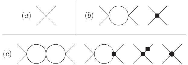
Figure 3: Feynman graphs contributing to $\pi\pi$ scattering at (a) $\mathcal{O}(p^{2})$, (b) $\mathcal{O}(p^{4})$, (c) $\mathcal{O}(p^{6})$. The squares denote vertices from $\mathcal{L}^{(4)}$, the circle a vertex from $\mathcal{L}^{(6)}$.

4.2 Chiral symmetry breaking scale $\Lambda_{\chi}$

Although we have now established a power counting scheme that determines the power of momenta $p^{n}$ at which a certain diagram contributes, it is not yet clear compared to what scale these momenta are to be small. If we write the effective Lagrangian in the (slightly unconventional) form

$$\mathcal{L}_{\rm eff}=\dfrac{F^{2}}{4}\left\{\langle\partial_{\mu}U\partial^{\mu}U^{\dagger}\rangle+\dfrac{1}{{\Lambda_{\chi}^{2}}}\tilde{\mathcal{L}}^{(4)}+\dfrac{1}{{\Lambda_{\chi}^{4}}}\tilde{\mathcal{L}}^{(6)}+\ldots\right\}~{},$$ (35)

we need to know what the chiral symmetry breaking scale $\Lambda_{\chi}$ is. In other words, if we calculate higher-order corrections, what is their expected size $\propto p^{2}/\Lambda_{\chi}^{2}$, $\propto M_{\pi}^{2}/\Lambda_{\chi}^{2}$?

As a first argument, let us compare the two $\mathcal{O}(p^{4})$ contributions to $\pi\pi$ scattering in Fig. 3(b) in a generic manner:

	$\propto~{}\displaystyle{\int}\dfrac{d^{4}p}{(2\pi)^{4}}\dfrac{1}{(p^{2})^{2}}\biggl{(}\dfrac{p^{2}}{F^{2}}\biggr{)}^{2}\stackrel{{\scriptstyle\rm dim.reg}}{{\propto}}\dfrac{p^{4}}{(4\pi)^{2}F^{4}}\log\mu$  ,
	$\propto~{}\dfrac{F^{2}}{\Lambda_{\chi}^{2}}\dfrac{p^{4}}{F^{4}}\ell_{i}(\mu)~{}.$

The scale-dependent “low-energy constant” (LEC) $\ell_{i}(\mu)$ multiplying the tree-level graph compensates for the logarithmic scale dependence of the loop graph (as evaluated in dimensional regularisation). Naturally, the finite part of $\ell_{i}(\mu)$ should not be expected to be smaller than the shift induced by a change in the scale $\mu$, therefore

$$\Lambda_{\chi}\approx 4\pi F\approx 1.2~{}{\rm GeV}~{}.$$ (36)

As a second argument, we have to remember that we have constructed an effective theory for Goldstone bosons, which are the only dynamical degrees of freedom. The effective theory must fail once the energy reaches the resonance region, hence for $p^{2}/\Lambda_{\chi}^{2}\approx p^{2}/M_{\rm res}^{2}\approx 1$. The resonance masses are channel-dependent, the lightest being $M_{\rm res}=M_{\rho}=770$ MeV, and typically $M_{\rm res}\approx 1$ GeV, therefore this second estimate is roughly consistent with $\Lambda_{\chi}=4\pi F$.

4.3 The chiral Lagrangian at higher orders

The number of independent terms and corresponding low-energy constants increases rapidly at higher orders. In fact, for chiral SU($n$), $n=(2,3)$,

$\mathcal{L}^{(2)}$	contains	(2, 2)	constants	($F$, $B$),
$\mathcal{L}^{(4)}$	contains	(7, 10)	constants	[18, 19],
$\mathcal{L}^{(6)}$	contains	(53, 90)	constants	[20]

(discounting so-called contact terms that depend on external fields only). As an example, we display $\mathcal{L}^{(4)}$ explicitly for chiral SU(3):

$$\mathcal{L}^{(4)}\!\! = \!\!{L_{1}}\langle D_{\mu}U^{\dagger}D^{\mu}U\rangle^{2}+{L_{2}}\langle D_{\mu}U^{\dagger}D_{\nu}U\rangle\langle D^{\mu}U^{\dagger}D^{\nu}U\rangle$$ (37)

$$+ \!\!{L_{3}}\langle D_{\mu}U^{\dagger}D^{\mu}UD_{\nu}U^{\dagger}D^{\nu}U\rangle+{L_{4}}\langle D_{\mu}U^{\dagger}D^{\mu}U\rangle\langle\chi^{\dagger}U+\chi U^{\dagger}\rangle$$

$$+ \!\!{L_{5}}\langle D_{\mu}U^{\dagger}D^{\mu}U(\chi^{\dagger}U+\chi U^{\dagger})\rangle+{L_{6}}\langle\chi^{\dagger}U+\chi U^{\dagger}\rangle^{2}$$

$$+ \!\!{L_{7}}\langle\chi^{\dagger}U-\chi U^{\dagger}\rangle^{2}+{L_{8}}\langle\chi^{\dagger}U\chi^{\dagger}U+\chi U^{\dagger}\chi U^{\dagger}\rangle$$

$$- \!\!i\,{L_{9}}\langle F_{R}^{\mu\nu}D_{\mu}UD_{\nu}U^{\dagger}+F_{L}^{\mu\nu}D_{\mu}U^{\dagger}D_{\nu}U\rangle+{L_{10}}\langle U^{\dagger}F_{R}^{\mu\nu}UF_{L\mu\nu}\rangle~{}.~{}$$

Here, $\chi=2B(s+ip)$ collects (pseudo)scalar source terms, where $s$ contains the quark mass matrix, $s=\mathcal{M}+\ldots\,$; vector and axial currents are combined as $r_{\mu}=v_{\mu}+a_{\mu}$, $l_{\mu}=v_{\mu}-a_{\mu}$, from which one can form field strength tensors, $F_{R}^{\mu\nu}=\partial^{\mu}r^{\nu}-\partial^{\nu}r^{\mu}-i[r^{\mu},r^{\nu}]$, and similarly $F_{L}^{\mu\nu}$. We note that $L_{1-3}$ multiply structures containing four derivatives; $L_{4,5}$ those with two derivatives and one quark mass term; the structures corresponding to $L_{6-8}$ scale with the quark masses squared. $L_{9,10}$ only contribute to observables with external vector and axial vector sources. The seven similar constants in SU(2) that we will also partly use later are conventionally denoted by ${\ell_{i}}$, $i=1,\ldots,7$.

4.4 The physics behind the low-energy constants

To better understand the role of the low-energy constants and the physics they incorporate, let us consider massive states (resonances) that are “integrated out” of the theory, i.e. no dynamical degrees of freedom for energies below $\Lambda_{\chi}$:

$$\mathcal{L}[U,\partial U,\ldots,{H}]~{}\stackrel{{\scriptstyle\Lambda}}{{\longrightarrow}}~{}\mathcal{L}_{\rm eff}[U,\partial U,\ldots]~{}.$$ (38)

A Lagrangian for the resonance fields, coupled to source terms, is of the form

$$\mathcal{L}[H]=\frac{1}{2}\left(\partial_{\mu}H\partial^{\mu}H-M_{H}^{2}H^{2}\right)+JH~{},$$ (39)

where $J$ is a current formed of light degrees of freedom. In the path integral, we can use the fact the the heavy particle propagator $\Delta_{H}(x-y)$ is peaked for small separations $|x-y|$,

$$S_{\rm eff}[J]=-\frac{1}{2}\int d^{4}xd^{4}y\,J(x)\Delta_{H}(x-y)J(y)\simeq\int d^{4}x\frac{1}{2{M_{H}^{2}}}J(x)J(x)+\ldots~{},$$ (40)

i.e. this generates local higher-order operators, with the couplings proportional to the inverse heavy masses. We conclude therefore that the effects of higher-mass states on the Goldstone boson interactions are hidden in the low-energy constants of higher-order terms in the chiral Lagrangian.

As an example, we consider the pion vector form factor $F_{\pi}^{V}(s)$, defined as

$$\langle\pi^{a}(p)\pi^{b}(p^{\prime})\,|\,\bar{q}\frac{\tau^{3}}{2}\gamma_{\mu}q\,|\,0\rangle=i\epsilon^{a3b}(p^{\prime}-p)_{\mu}F_{\pi}^{V}(s)~{},\quad s=(p+p^{\prime})^{2}~{}.$$ (41)

In ChPT at $\mathcal{O}(p^{4})$, there are loop diagrams contributing to $F_{\pi}^{V}(s)$ as well as a tree graph proportional to the low-energy constant $\bar{\ell}_{6}$. Expanding $F_{\pi}^{V}(s)$ for small $s$, we find for the radius term $\langle r^{2}\rangle_{\pi}^{V}$

$$F_{\pi}^{V}(s)=1+\frac{1}{6}{\langle r^{2}\rangle_{\pi}^{V}}s+\mathcal{O}(s^{2})~{},\quad\langle r^{2}\rangle_{\pi}^{V}=\frac{1}{(4\pi F_{\pi})^{2}}({\bar{\ell}_{6}}-1)~{}.$$ (42)

Now consider the contribution of the $\rho$-resonance (see e.g. [21] for how to treat vector mesons in the context of chiral Lagrangians) to this form factor,

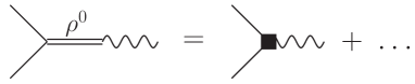
Figure 4: The contribution of the $\rho$-resonance to the pion vector form factor can, at small $t$, be represented by a point-like counterterm.

as shown in Fig. 4. Expanding the $\rho$ propagator for $s\ll M_{\rho}^{2}$,

$$\frac{s}{M_{\rho}^{2}-s}=\frac{s}{M_{\rho}^{2}}\biggl{(}1+\frac{s}{M_{\rho}^{2}}+\ldots\biggr{)}~{},$$ (43)

we find that identifying the leading term with the $\bar{\ell}_{6}$ contribution reproduces the empirical value for $\bar{\ell}_{6}$ nicely. This is a modern version of the time-honoured concept of “vector meson dominance”: where allowed by quantum numbers, the numerical values of LECs are dominated by the contributions of vector resonances [22, 23].

4.5 The pion mass to $\mathcal{O}(p^{4})$

As an example for a higher-order calculation, we consider the pion mass up to $\mathcal{O}(p^{4})$. The necessary diagrams are shown in Fig. 5.

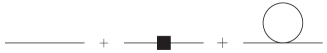
Figure 5: Diagrams contributing to the pion self energy up to $\mathcal{O}(p^{4})$.

We find for the pion propagator

$$\delta^{ab}\Delta(p) = i\int d^{4}xe^{ipx}\langle 0|T\phi^{a}(x)\phi^{b}(0)|0\rangle~{},$$

$$\Delta(p) = \dfrac{Z}{M_{\pi}^{2}-p^{2}}\;(+{\rm 2~{}loops})~{}.$$ (44)

The physical pion mass is given, to this order, by

$$M_{\pi}^{2}=M^{2}+\frac{M^{2}}{2F^{2}}I+\frac{2{\ell_{3}}}{F^{2}}M^{4}~{},$$ (45)

where $M^{2}=B(m_{u}+m_{d})$, and the loop integral

$$I~{}=~{}\frac{1}{i}\int\frac{d^{4}l}{(2\pi)^{4}}\frac{1}{M^{2}-l^{2}}$$ (46)

is actually divergent and has to be regularised. A “good” regularisation scheme, for our purposes, is dimensional regularisation, as it preserves all symmetries (which is much more difficult to achieve using a cutoff, say). In $d$ dimensions, we find

$$I~{}\to~{}\frac{1}{i}\int\frac{d^{d}l}{(2\pi)^{d}}\frac{1}{M^{2}-l^{2}}~{}=~{}\frac{M^{d-2}}{(4\pi)^{d/2}}\Gamma\Bigl{(}1-\frac{d}{2}\Bigr{)}~{},$$ (47)

which is finite for $d\neq 2,\,4,\,6,\ldots\,$, but still divergent for $d=4$:

$$I~{}\to~{}\frac{M^{2}}{8\pi^{2}}\left\{{\frac{1}{d-4}}+\log\frac{M}{\mu}+\ldots\right\}~{}.$$

We now tune $\ell_{3}$ such as to absorb this divergence (as well as the $\mu$-dependence):

$$\ell_{3}~{}\to~{}-\frac{1}{32\pi^{2}}\left({\frac{1}{d-4}}+\log\frac{M}{\mu}+\frac{\bar{\ell}_{3}}{2}\right)~{},$$ (48)

such that $\bar{\ell}_{3}$ contains the finite part of $\ell_{3}$, and find

$$M_{\pi}^{2}~{}=~{}M^{2}-\dfrac{M^{4}}{32\pi^{2}F^{2}}{\bar{\ell}_{3}}+\mathcal{O}(M^{6})~{}.$$ (49)

A few comments on renormalisation as we just saw it at work for the first time are in order. The required counterterm to cancel the divergence stems from $\mathcal{L}^{(4)}$; it is not sufficient to tune $\mathcal{L}^{(2)}$ parameters. This is typical for a non-renormalisable theory: going to to higher and higher orders, we need more and more counterterms. However, the fact that the theory is non-renormalisable does not mean it is non-calculable, the only disadvantage is the increasing number of LECs when calculating higher-order corrections. It is important to note furthermore that the LECs feature in different observables, and that their divergent parts and scale dependences are always the same. The renormalisation can be performed on the level of the generating functional in a manifestly chirally invariant way, and the $\beta$-functions of the $\ell_{i}$ [18], $L_{i}$ [19] (and also of $\mathcal{L}^{(6)}$ LECs [24]) are known. The cancellation of divergences and scale dependence therefore serves as a powerful check on any specific calculations.

4.6 Quark mass expansion of the pion mass revisited

The expression (49) provides a correction to the Gell-Mann–Oakes–Renner relation: generically, it is of the form

$$M_{\pi}^{2}=B(m_{u}+m_{d})+A(m_{u}+m_{d})^{2}+\mathcal{O}(m_{q}^{3})~{}.$$ (50)

Apart from naive order-of-magnitude expectations, how do we actually know that the leading term dominates? What if $\bar{\ell}_{3}$ turns out to be anomalously large? The consequences of this possibility were explored under the label of “generalised ChPT”, which employs a different power counting scheme [25]. The essential question in order to determine the size of second-order corrections in the quark mass expansion of the pion mass is therefore: how can we learn something about $\bar{\ell}_{3}$?

4.7 $\pi\pi$ scattering at next-to-leading order

It turns out the process to study is, once more, $\pi\pi$ scattering. The $\pi\pi$ scattering lengths are known to next-to-next-to-leading order [26], the $\mathcal{O}(p^{4})$ corrections for the $I=0$ scattering length are of the form [18]

$$a_{0}^{0} = \frac{7M_{\pi}^{2}}{32\pi F_{\pi}^{2}}\Bigl{\{}1+\epsilon+\mathcal{O}(M_{\pi}^{4})\Bigr{\}}~{},$$

$$\epsilon = \frac{5M_{\pi}^{2}}{84\pi^{2}F_{\pi}^{2}}\left({\bar{\ell}_{1}}+2{\bar{\ell}_{2}}+\frac{3}{8}{\bar{\ell}_{3}}+\frac{21}{10}{\bar{\ell}_{4}}+\frac{21}{8}\right)~{}.$$ (51)

There are two different types of LECs in the expression (51). $\bar{\ell}_{1}$, $\bar{\ell}_{2}$ come with structures containing four derivatives (like $L_{1-3}$ in (37)), i.e. they survive in the chiral limit and can be determined from the momentum dependence of the $\pi\pi$ scattering amplitude, namely from $d$-waves. $\bar{\ell}_{3}$, $\bar{\ell}_{4}$ however are symmetry breaking terms that specify the quark mass dependence (comparable to $L_{4,5}$ in (37)), therefore they cannot be determined from $\pi\pi$ scattering alone.

One additional observable to consider is the scalar form factor of the pion $\Gamma(s)$, which is defined as

$$\langle\pi^{a}(p)\pi^{b}(p^{\prime})\,|\,\hat{m}(\bar{u}u+\bar{d}d)\,|\,0\rangle=\delta^{ab}{\Gamma(s)}~{},\quad s=(p+p^{\prime})^{2}~{}.$$ (52)

At tree level, one has ${\Gamma(s)}=2B\hat{m}=M_{\pi}^{2}+\mathcal{O}(p^{4})$ in accordance with the Feynman-Hellman theorem, ${\Gamma(0)}=\langle\pi\,|\,\hat{m}\,\bar{q}q\,|\,\pi\rangle=\hat{m}\,{\partial M_{\pi}^{2}}/{\partial\hat{m}}\,.$ At next-to-leading order, one defines the scalar radius $\langle r^{2}\rangle_{\pi}^{S}$ according to

$${\Gamma(s)} = \Gamma(0)\left\{1+\frac{1}{6}{\langle r^{2}\rangle_{\pi}^{S}}s+\mathcal{O}(s^{2})\right\}~{},$$

$${\langle r^{2}\rangle_{\pi}^{S}} = \frac{3}{8\pi^{2}F_{\pi}^{2}}\left({\bar{\ell}_{4}}-\frac{13}{12}\right)+\mathcal{O}(M_{\pi}^{2})~{},$$ (53)

therefore the scalar radius is directly linked to $\bar{\ell}_{4}$. Although the scalar form factor is not directly experimentally accessible, one can analyse $\Gamma(s)$ in dispersion theory and extract $\langle r^{2}\rangle_{\pi}^{S}$ that way.

If we plug in the low-energy theorems and eliminate $\bar{\ell}_{1}$, $\bar{\ell}_{2}$, $\bar{\ell}_{4}$ in favour of the $d$-wave scattering lengths $a_{2}^{I=0,2}$ and the scalar radius, we can rewrite $\epsilon$ in (51) as

$$\epsilon=\frac{M_{\pi}^{2}}{3}{\langle r^{2}\rangle_{\pi}^{S}}+\frac{200\pi}{7}F_{\pi}^{2}M_{\pi}^{2}\left({a_{2}^{0}}+2{a_{2}^{2}}\right)-\frac{M_{\pi}^{2}}{672\pi^{2}F_{\pi}^{2}}\left(15{\bar{\ell}_{3}}-353\right)~{}.$$ (54)

Therefore all we need to do is to measure $a_{0}^{0}$ and extract $\bar{\ell}_{3}$ from the above relation. This will tell us how much of $M_{\pi}^{2}$ is due to the linear term in the quark mass expansion.

4.8 Experiments on $\pi\pi$ scattering

How can the $\pi\pi$ scattering lengths be measured? We wish to briefly comment on four different possibilities to extract information on the $\pi\pi$ interaction at low energies: pion reactions on nucleons, in particular $\pi N\to\pi\pi N$; so-called $K_{e4}$ decays $K^{+}\to\pi^{+}\pi^{-}e^{+}\nu_{e}$ [27, 28]; the cusp phenomenon in $K^{+}\to\pi^{+}\pi^{0}\pi^{0}$ [29]; and the lifetime of pionium [30].

$\pi N\to\pi\pi N$

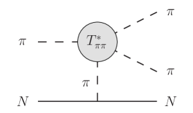
Figure 6: One-pion exchange contributions to $\pi N\to\pi\pi N$.

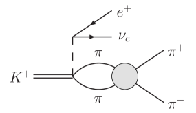
Figure 7: $\pi\pi$ rescattering in $K_{e4}$ decays.

As shown schematically in Fig. 7, the process $\pi N\to\pi\pi N$ receives contributions from graphs containing the off-shell $\pi\pi$ amplitude $T_{\pi\pi}^{*}$, therefore it ought to be sensitive to $\pi\pi$ interactions. In order to isolate the one-pion-exchange contribution, one has to extrapolate to the pion pole at $t=M_{\pi}^{2}$, which is outside the physical region; this procedure is not without difficulties, and the data obtained thereof tend to be at relatively high energies, so it does not give direct access to scattering lengths without further theoretical input; see [31] for a ChPT-based analysis.

$K^{+}\to\pi^{+}\pi^{-}e^{+}\nu_{e}$

Why is it possible to measure $\pi\pi$ scattering in such a kaon decay process? The first, naive explanation, is that the pions undergo final-state interactions, see Fig. 7, and they are the only strongly interacting particles in the final state, therefore they ought to be sensitive to this interaction. The more educated explanation is that $K_{e4}$ decays can be described by form factors, which share the phases of $\pi\pi$ interaction due to Watson’s final state theorem [32]. It can be shown [33] that the interference between $s$- and $p$-waves can be unambiguously extracted,

$$\delta_{0}^{0}(E_{\pi\pi})-\delta_{1}^{1}(E_{\pi\pi})~{},$$

and as $E_{\pi\pi}$ is kinematically restricted to be smaller than $M_{K}$, these phases are measured close to threshold.

Cusp in $K^{+}\to\pi^{+}\pi^{0}\pi^{0}$

In a measurement of the kaon decay process $K^{+}\to\pi^{+}\pi^{0}\pi^{0}$, the NA48/2 collaboration has detected a cusp phenomenon, i.e. a sudden change in slope, in the invariant mass spectrum of the $\pi^{0}\pi^{0}$ pair at$M_{\pi^{0}\pi^{0}}=2M_{\pi^{+}}$ [29].

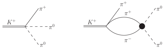
Figure 8: “Direct” and “rescattering” contributions to $K^{+}\to\pi^{+}\pi^{0}\pi^{0}$.

As suggested in Fig. 8, this phenomenon can be explained by an interference effect between “direct” tree graphs for $K^{+}\to\pi^{+}\pi^{0}\pi^{0}$ and a $K^{+}\to\pi^{+}\pi^{+}\pi^{-}$ decay, followed by $\pi^{+}\pi^{-}\to\pi^{0}\pi^{0}$ rescattering. The one-loop graph has a smooth part plus a part $v_{+-}(s)$, where

$$v_{+-}(s)=\left\{\begin{array}[]{ll}-\frac{1}{16\pi}\sqrt{\frac{4M_{\pi^{\pm}}^{2}}{s}-1}~{},&s<4M_{\pi^{\pm}}^{2}~{},\\[5.69054pt] \frac{i}{16\pi}\sqrt{1-\frac{4M_{\pi^{\pm}}^{2}}{s}}~{},&s>4M_{\pi^{\pm}}^{2}~{}.\end{array}\right.$$ (55)

Below the $\pi^{+}\pi^{-}$ threshold, the loop graph is real and interferes directly with the tree contributions, while above threshold, it does not. Due to the square-root behaviour of $v_{+-}(s)$, a cusp is seen [34, 35]. The strength of this cusp is proportional to the scattering amplitude for $\pi^{+}\pi^{-}\to\pi^{0}\pi^{0}$ at threshold, hence a combination of $\pi\pi$ scattering lengths.

This behaviour is complicated at two-loop order as in contrast to $K_{e4}$, there are three strongly interacting particles in the final state [35, 36, 37]; in addition, virtual photons further modify the cusp structure. Nevertheless, the high statistics available in the experimental data in principle allow for a very precise determination of the scattering lengths, and the appropriate theoretical accuracy has to be provided.

Pionium lifetime

Pionium is a hadronic atom, a $\pi^{+}\pi^{-}$ system bound by electromagnetism. The energy levels of this system can in principle be calculated as in quantum mechanics for the hydrogen atom, however, they are perturbed by the strong interactions: the ground state is not stable, it decays according to

$$A_{\pi^{+}\pi^{-}}\to\pi^{0}\pi^{0},\,\gamma\gamma,\,\ldots~{}.$$

The decay width is given by the following (improved) Deser formula [38, 39] (further literature can be traced back from [40, 41]):

$$\Gamma = \frac{2}{9}\alpha^{3}p\,|{\mathcal{A}(\pi^{+}\pi^{-}\to\pi^{0}\pi^{0})_{\rm thr}}|^{2}(1+\epsilon)$$ (56)

$$= \frac{2}{9}\alpha^{3}p\,|{a_{0}^{0}-a_{0}^{2}}|^{2}(1+\delta)~{},$$

where $p$ is the momentum of the $\pi^{0}$ in the decay in the centre-of-mass frame, and $\epsilon$ and $\delta$ are numerical correction factors accounting for isospin violation effects beyond leading order, $\delta=0.058\pm 0.012$ [42]. Taking information on the scattering lengths from elsewhere, one can predict the pionium lifetime as

$$\tau=(2.9\pm 0.1)\times 10^{-15}s~{}.$$ (57)

Ultimately, one however wants to turn the argument around, measure the lifetime and extract $a_{0}^{0}-a_{0}^{2}$. The corresponding experimental efforts are undertaken by the DIRAC collaboration, first results have been obtained [30].

Result on $\bar{\ell}_{3}$

For reasons of brevity, we just compare to the BNL-865 result for $a_{0}^{0}$ [27],

$$a_{0}^{0}=0.216\pm 0.013_{\rm stat}\pm 0.004_{\rm syst}\pm 0.005_{\rm theo}~{}.$$ (58)

For an up-to-date compilation of the various experimental results, see e.g. [43] and references therein. From (58), one can extract a value for $\bar{\ell}_{3}\approx 6\pm 10$, which is compatible with the original estimate in [18] as well as lattice determinations (see [44] and the discussion in [43]). For the central value, the subleading correction for $M_{\pi}^{2}$ in (49) amounts to a mere 4%, therefore even from this seemingly rather loose bound, on can conclude that the leading term in the quark mass expansion of the pion mass dominates by far [45].

4.9 On the size of the corrections in $a_{0}^{0}$

If we remember the tree-level result for $a_{0}^{0}$ (31), $a_{0}^{0}({\rm tree})=0.16$, the experimental result (58) seems somewhat surprising: higher-order corrections are of the order of $30\%$, rather than of the order of $M_{\pi}^{2}/(4\pi F_{\pi})^{2}\approx 2\%$. In order to understand this, we have to have another look at $\epsilon$ in (51). The $\bar{\ell}_{i}$ contain chiral logarithms, $\bar{\ell}_{i}\to-\log M_{\pi}^{2}$; collecting these together, $\epsilon$ contains logarithmic terms

$$\epsilon~{}=~{}-\frac{9M_{\pi}^{2}}{32\pi^{2}F_{\pi}^{2}}{\log\frac{M_{\pi}^{2}}{\mu^{2}}}$$ (59)

which, estimated at a scale $\mu=1$ GeV, alone amount to 25%. We conclude that chiral logarithms potentially enhance higher-order corrections, and that the isoscalar $s$-wave $\pi\pi$ scattering length contains chiral logarithms with rather large coefficients, therefore corrections to the tree-level result are sizeable.

4.10 Quark mass ratios revisited

As another application of ChPT beyond leading order, we want to briefly revisit the ratios of the light quark masses. Forming dimensionless ratios, it turns out that one can write the $\mathcal{O}(p^{4})$ corrections in the form [19]

$$\frac{M_{K}^{2}}{M_{\pi}^{2}} = \frac{m_{s}+\hat{m}}{m_{u}+m_{d}}\Bigl{\{}1+{\Delta_{M}}+\mathcal{O}(m_{q}^{2})\Bigr{\}}~{},$$

$$\frac{(M_{K^{0}}^{2}-M_{K^{+}}^{2})_{\rm strong}}{M_{K}^{2}-M_{\pi}^{2}} = \frac{m_{d}-m_{u}}{m_{s}-\hat{m}}\Bigl{\{}1+{\Delta_{M}}+\mathcal{O}(m_{q}^{2})\Bigr{\}}~{},$$

$${\rm where}\quad{\Delta_{M}} = \frac{8(M_{K}^{2}-M_{\pi}^{2})}{F_{\pi}^{2}}(2L_{8}-L_{5})+{\rm chiral~{}logs}~{}.$$ (60)

The double ratio $Q^{2}$ is therefore particularly stable with respect to higher-order corrections,

$$Q^{2}=\frac{m_{s}^{2}-\hat{m}^{2}}{m_{d}^{2}-m_{u}^{2}}=\frac{M_{K}^{2}}{M_{\pi}^{2}}\frac{M_{K}^{2}-M_{\pi}^{2}}{(M_{K^{0}}^{2}-M_{K^{+}}^{2})_{\rm strong}}\Bigl{\{}1+\mathcal{O}(m_{q}^{2})\Bigr{\}}~{}.$$ (61)

(61) can be rewritten in the form of an ellipse equation for the quark mass ratios $m_{u}/m_{d}$, $m_{s}/m_{d}$ (Leutwyler’s ellipse [46]),

$$\left(\frac{m_{u}}{m_{d}}\right)^{2}+\frac{1}{{Q^{2}}}\left(\frac{m_{s}}{m_{d}}\right)^{2}=1~{}.$$ (62)

We can use Dashen’s theorem (26) to determine $(M_{K^{0}}^{2}-M_{K^{+}}^{2})_{\rm strong}$ and therefore $Q$, with the result

$$Q_{\rm Dashen}=24.2~{}.$$ (63)

However, corrections to Dashen’s theorem of $\mathcal{O}(e^{2}m_{q})$ are potentially large, different models yield a range [47]

$$1~{}\lesssim~{}(M_{K^{+}}^{2}-M_{K^{0}}^{2})_{\rm em}/(M_{\pi^{+}}^{2}-M_{\pi^{0}}^{2})_{\rm em}~{}\lesssim~{}2.5~{},$$ (64)

inducing a rather large uncertainty in $Q$, $20.6\lesssim Q\lesssim 24.2$. It would therefore be most desirable to obtain information on $Q$ independent on meson mass relations. One such source will be introduced in the following subsection.

4.11 $\eta\to 3\pi$

The $\eta$ meson has isospin $I=0$, while three pions with angular momentum 0 cannot have $I=0$, but only $I=1$. $\eta\to 3\pi$ is therefore an isospin violating decay. Using the leading chiral Lagrangian $\mathcal{L}^{(2)}$ (including isospin breaking), the tree amplitude for $\eta\to\pi^{+}\pi^{-}\pi^{0}$ can be calculated to be

$$A(s,t,u)=\frac{B({m_{u}-m_{d}})}{3\sqrt{3}F_{\pi}^{2}}\left\{1+\frac{3(s-s_{0})}{M_{\eta}^{2}-M_{\pi}^{2}}\right\}~{},$$ (65)

where $s=(p_{\eta}-p_{\pi^{0}})^{2}$, $t=(p_{\eta}-p_{\pi^{+}})^{2}$, $u=(p_{\eta}-p_{\pi^{-}})^{2}$, $3s_{0}=s+t+u=M_{\eta}^{2}+2M_{\pi^{+}}^{2}+M_{\pi^{0}}^{2}$. For $\eta\to 3\pi^{0}$, one finds the amplitude $A(s,t,u)+A(t,u,s)+A(u,s,t)$, with $A$ as given in (65). We note that the electromagnetic term (25) does not contribute [48]. Terms of order $e^{2}m_{q}$ were found to be very small [49], therefore $\eta\to 3\pi$ (potentially) allows for a much cleaner access to $m_{u}-m_{d}$ than the meson masses. We can rewrite $A(s,t,u)$ explicitly in terms of $Q^{2}$,

$$A(s,t,u) = \frac{1}{{Q^{2}}}\frac{M_{K}^{2}}{M_{\pi}^{2}}\left(M_{\pi}^{2}-M_{K}^{2}\right)\frac{M(s,t,u)}{3\sqrt{3}F_{\pi}^{2}}~{},$$

$$M(s,t,u) = \frac{3s-4M_{\pi}^{2}}{M_{\eta}^{2}-M_{\pi}^{2}}\quad{\rm(at~{}leading~{}order)\,.}$$ (66)

Problems here arise from the fact that there are strong final-state interactions among the three pions: the one-loop corrections increase the width by a factor of 2.5,

$$\textrm{tree:}\quad\Gamma(\eta\to\pi^{+}\pi^{-}\pi^{0}) = 66~{}{\rm eV}~{},$$

$$\textrm{one-loop:}\quad\Gamma(\eta\to\pi^{+}\pi^{-}\pi^{0}) = 160\pm 50~{}{\rm eV}\quad\cite[cite]{[\@@bibref{}{GLeta}{}{}]}~{},$$ (67)

and even higher-order corrections are not negligible. Furthermore, there are partially contradictory experimental results (in particular on Dalitz plot parameters). This is therefore still a process of current interest, with strong ongoing experimental efforts for both final states [51].

The combined information on $Q$ as deduced from various corrections to Dashen’s theorem is shown in Fig. 9, together with two results obtained from studies of $\eta\to 3\pi$ [52, 53] (see also the discussion in [54]).

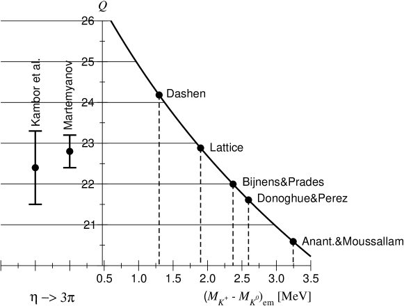
Figure 9: Various results on $Q$ [47, 52, 53]. The figure is inspired by [46].

Even with $Q$ fixed, additional constraints are needed to find the position on the ellipse. Two possibilities are information on $\eta\eta^{\prime}$ mixing, which, together with large–$N_{c}$ arguments, leads to a determination of $\Delta_{M}$ in (60). Alternatively, the ratio $R=(m_{s}-\hat{m})/(m_{d}-m_{u})$ can be extracted from baryon masses [55].

5 Chiral perturbation theory with baryons

So far, we have considered an effective field theory exclusively for (pseudo) Goldstone bosons. Perhaps the most important extension of this theory is the inclusion of nucleons or the baryon ground state octet in chiral SU(2) and SU(3), respectively. The problem, as we shall see later, is that the nucleon mass is a new, heavy mass scale that does not vanish in the chiral limit,

$${\lim_{m_{q}\to 0}m_{N}\approx m_{N}}~{}.$$

The idea for their incorporation in the theory is to view nucleons as (massive) matter fields coupled to pions and external sources. Their 3-momenta ought to remain small, of the order of $M_{\pi}$, in all processes. The number of baryons is therefore conserved, we consider no baryon–antibaryon creation/annihilation. In particular, in these lectures, we confine ourselves to processes with exactly one baryon.

For the construction of the meson-baryon Lagrangian, we proceed as before: we choose a suitable representation and transformation law for baryons under ${\rm SU}(N)_{L}\times{\rm SU}(N)_{R}$, and organise the effective Lagrangian according to an increasing number of momenta.

It turns out to be convenient to introduce a new field $u$ for the Goldstone boson fields according to $u^{2}=U$, which transforms as

$$u~{}\longmapsto~{}\sqrt{LUR^{\dagger}}=L\,u\,{K^{\dagger}(L,R,U)}={K(L,R,U)}\,u\,R^{\dagger}~{}.$$ (68)

Here, ${K(L,R,U)}\in{\rm SU}(N)$ is the so-called compensator field, that depends in a non-trivial way on $L$, $R$, and $U$. For SU$(N)_{V}$ transformations ($L=R$), (68) obviously reduces to $K(L,R,U)=L=R$.

A particularly convenient representation for nucleons and baryons is given by the following:

$$\psi=\biggl{(}\!\begin{array}[]{c}p\\ n\end{array}\!\biggr{)} \longmapsto \,{\psi^{\prime}=K\psi}~{},$$ (71)

$$B=\left(\!\begin{array}[]{ccc}\frac{\Sigma^{0}}{\sqrt{2}}+\frac{\Lambda}{\sqrt{6}}&\Sigma^{+}&p\\ \Sigma^{-}&-\frac{\Sigma^{0}}{\sqrt{2}}+\frac{\Lambda}{\sqrt{6}}&n\\ \Xi^{-}&\Xi^{0}&-\frac{2\Lambda}{\sqrt{6}}\end{array}\!\right) \longmapsto {B^{\prime}=KBK^{-1}}~{}.$$ (75)

We introduce a covariant derivative $D^{\mu}=\partial^{\mu}+\Gamma^{\mu}$ with the chiral connection $\Gamma^{\mu}$ (vector)

$$\Gamma^{\mu}=\frac{1}{2}\bigl{(}u^{\dagger}(\partial^{\mu}-i\,r^{\mu})u+u(\partial^{\mu}-i\,l^{\mu})u^{\dagger}\bigr{)}$$ (76)

that transforms according to $\Gamma^{\mu}\mapsto K\Gamma^{\mu}K^{\dagger}-(\partial^{\mu}K)K^{\dagger}$, such that the covariant derivative has the expected transformation behaviour

$$D^{\mu}\psi\longmapsto KD^{\mu}\psi~{}.$$

Furthermore, we shall use the chiral vielbein (axial vector)

$$u^{\mu}=i\bigl{(}u^{\dagger}(\partial^{\mu}-i\,r^{\mu})u-u(\partial^{\mu}-i\,l^{\mu})u^{\dagger}\bigr{)}$$ (77)

that transforms according to $u^{\mu}\mapsto Ku^{\mu}K^{\dagger}$. Finally, we can rewrite the (pseudo)scalar source term $\chi=2B(s+i\,p)=2B{\mathcal{M}}+\ldots$ as

$$\chi_{+}=u^{\dagger}\chi u^{\dagger}+u\chi^{\dagger}u~{},$$ (78)

such that $\chi_{+}\mapsto K\chi_{+}K^{\dagger}$, and all the constitutive elements of the chiral Lagrangian transform with the compensator field $K$.

5.1 The leading-order chiral meson-baryon Lagrangian

We are now in the position to write down the leading-order meson-baryon Lagrangian, both for chiral SU(2) and SU(3):

$$\mathcal{L}^{(1)}_{\pi N}\!\! = \!\!\bar{\psi}\left(i\gamma_{\mu}D^{\mu}-{m}+\frac{{g_{A}}}{2}\gamma_{\mu}\gamma_{5}u^{\mu}\right)\psi~{},$$ (79)

$$\mathcal{L}^{(1)}_{\phi B}\!\! = \!\!\langle\bar{B}\left(i\gamma_{\mu}D^{\mu}-{m}\right)B\rangle+\frac{D/F}{2}\langle\bar{B}\gamma_{\mu}\gamma_{5}[u^{\mu},B]_{\pm}\rangle~{}.$$ (80)

While in meson ChPT, the Lagrangians come only in even powers of derivatives or momenta, odd powers of momenta are allowed in the meson-baryon sector due to the presence of spin (or, more general, Dirac structures):

$$\mathcal{L}_{\pi N}=\mathcal{L}_{\pi N}^{(1)}+\mathcal{L}_{\pi N}^{(2)}+\mathcal{L}_{\pi N}^{(3)}+\mathcal{L}_{\pi N}^{(4)}+\ldots~{}.$$

The new parameters of $\mathcal{L}^{(1)}_{\pi N}$ comprise $m$, the nucleon (baryon) mass in the chiral limit; $g_{A}$ (in SU(2)), which, upon expansion of $u_{\mu}=2a_{\mu}+\mathcal{O}(\pi)$, can be identified with the axial vector coupling that is known from neutron beta decay, $g_{A}=1.26$; or $D/F$, the two axial vector couplings in SU(3), which can be determined from semileptonic hyperon decays and have to fulfil the SU(2) constraint $D+F=g_{A}$ ($D\approx 0.80,F\approx 0.46$).

5.2 Goldberger–Treiman relation

As a first consequence of (79), we want to derive the so-called Goldberger–Treiman relation. Setting external sources to zero, $v_{\mu}=a_{\mu}=0$, and expanding in powers of the pion field, we find $u_{\mu}=-\partial_{\mu}\pi/F_{\pi}+\mathcal{O}(\pi^{3})$ for the chiral vielbein, which results in the $\pi NN$ vertex

$$\mathcal{L}^{(1)}_{\pi N}\to-\frac{g_{A}}{2F_{\pi}}{\bar{\psi}}\gamma^{\mu}\gamma_{5}{\partial_{\mu}\pi\psi}~{}.$$ (81)

The corresponding Feynman rule looks as follows:

$\dfrac{g_{A}}{2F_{\pi}}\!\not\!q\gamma_{5}\vec{\tau}~{}\doteq~{}V_{\pi NN}~{}.$

We can deduce a $N\to\pi N$ transition amplitude

$$T_{\pi NN}=-i\bar{u}(p^{\prime})V_{\pi NN}u(p)=-i{\frac{g_{A}m_{N}}{F_{\pi}}}\bar{u}(p^{\prime})\gamma_{5}u(p)\vec{\tau}~{},$$

which, compared to the canonical amplitude $-i\,{g_{\pi N}}\bar{u}(p^{\prime})\gamma_{5}u(p)\vec{\tau}$, yields the relation

$$g_{\pi N}~{}=~{}\dfrac{g_{A}m_{N}}{F_{\pi}}~{}.$$ (82)

(82) is remarkable for relating weak ($g_{A}$) and strong ($F_{\pi}$) interaction quantities. Numerically it is rather well fulfilled in nature, $13.1\ldots 13.4=12.8$.

5.3 Weinberg’s power counting for the one-baryon sector

We can derive a similar power counting formula as in (34) for the one-baryon sector. The chiral dimension $\nu$ of an arbitrary $L$-loop diagram with $V_{d}^{\pi\pi}$ meson–meson vertices of order $d$ and $V_{d^{\prime}}^{\pi N}$ meson–baryon vertices of order $d^{\prime}$ is given by

$$\nu=2L+1+\sum_{d}V_{d}^{\pi\pi}(d-2)+\sum_{d^{\prime}}V_{d^{\prime}}^{\pi N}(d^{\prime}-1)~{}.$$ (83)

Note that $d\geq 2$, $d^{\prime}\geq 1$, such that the right hand side of (83) again consists of a sum of non-negative terms only. We conclude that at $\mathcal{O}(p^{1})$, $\mathcal{O}(p^{2})$, only tree diagrams contribute; tree plus one-loop diagrams enter at $\mathcal{O}(p^{3})$, $\mathcal{O}(p^{4})$; tree, one-loop, and two-loop diagrams can contribute to $\mathcal{O}(p^{5})$, $\mathcal{O}(p^{6})$, etc.

However, as it was noted in [56], in contrast to the meson sector, loop graphs do not necessarily obey the naive power counting rules as put forward in (83). The reason is that loop integrals cover all energy scales: while in the Goldstone boson sector, all mass scales are “small”, such that naive power counting has to work in a mass-independent regularisation scheme (like dimensional regularisation), there is a new mass scale in the nucleon sector, the nucleon mass $m_{N}\approx\Lambda_{\chi}\approx 1$ GeV. The loop integration then also picks up momenta $p\sim m_{N}$.

Schematically, the situation is depicted in Fig. 10: in contrast to the Goldstone boson sector, higher-order loop graphs in the meson-baryon theory renormalise lower-order couplings at each order in the loop expansion.

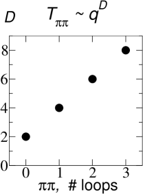
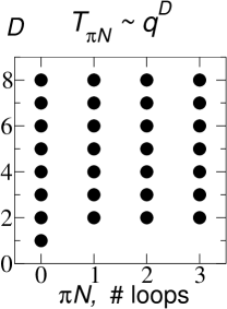
Figure 10: Schematic representation of loop contributions to chiral amplitudes in the Goldstone boson (left panel) and the meson-baryon (right panel) sector. The figure is inspired by [56].

In the following, we shall discuss two possible remedies to restore the features of naive power counting for meson-baryon ChPT.

5.4 Heavy-baryon ChPT

The first remedy goes by the name of heavy-baryon chiral perturbation theory (HBChPT) [57, 58]. It is constructed in close analogy to heavy-quark effective field theory: we decompose the baryon momentum into a large part proportional to the nucleon velocity, plus a small residual momentum according to

$$p_{\mu}~{}=~{}m_{N}v_{\mu}+l_{\mu}~{},\quad v^{2}=1~{},\quad v\cdot l\ll m_{N}~{}.$$ (84)

In the heavy-baryon limit, the nucleon propagator is then of the form

$$\frac{1}{p^{2}-m_{N}^{2}}~{}\to~{}\frac{1}{2m_{N}}\frac{1}{v\cdot l}+\mathcal{O}\bigl{(}1/m_{N}^{2}\bigr{)}~{}.$$

This procedure eliminates the mass scale $m_{N}$ from the propagator, which re-enters as a parametrical suppression factor. HBChPT is then a two-fold expansion in powers of $(p/\Lambda_{\chi})^{n}$ and $(p/m_{N})^{n}$, where $m_{N}\approx\Lambda_{\chi}$.

The nucleon field $\psi$ is decomposed into velocity eigenstates according to

$$H_{v}(x)=e^{im_{N}v\cdot x}P_{v}^{+}\psi(x)~{},\quad h_{v}(x)=e^{im_{N}v\cdot x}P_{v}^{-}\psi(x)~{},$$ (85)

where we have used the projectors $P_{v}^{\pm}=\frac{1}{2}(1\pm\!\!\not\!\!v)$ onto velocity eigenstates. $H_{v}$ represents the “big” components of the spinor at low energies, while $h_{v}$ are the “small” components. The exponential eliminates the large mass term from the time evolution of the field $H_{v}$. Written in terms of the new field $H_{v}$, the leading-order Lagrangian $\mathcal{L}_{\pi N}^{(1)}$ becomes

$$\mathcal{L}_{\pi N}^{(1)}=\bar{H}_{v}\bigl{(}iv\cdot D+g_{A}{S}\cdot u\bigr{)}H_{v}+\mathcal{O}\bigl{(}{1/m_{N}}\bigr{)}~{},$$ (86)

where we have introduced the Pauli-Lubanski spin vector ${S_{\mu}}=\frac{i}{2}\gamma_{5}\sigma_{\mu\nu}v^{\nu}$. We note that the nucleon mass does not occur in (86), and the Dirac structure is massively simplified. $1/m_{N}$ corrections can be constructed systematically on the Lagrangian level in analogy to Foldy–Wouthuysen transformations [58].

5.5 Infrared regularisation

The second procedure is called infrared regularisation [59] (see also [60, 61, 62] for variants of this approach). It is an alternative way to regularise loop integrals and allows for a manifestly covariant way to calculate loops in baryon ChPT.

Let us consider the (relativistic) nucleon self-energy graph in Fig. 11.

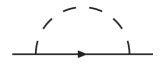
Figure 11: Nucleon self-energy graph. Full and dashed lines denote nucleon and pion, respectively.

Evaluated at threshold in $d$ dimensions, it yields the result

$$\frac{\Gamma(2-\frac{d}{2})}{(4\pi)^{d/2}(d-3)}\frac{{m_{N}^{d-3}}+{M_{\pi}^{d-3}}}{m_{N}+M_{\pi}}~{}.$$ (87)

We decompose (87) into two parts, the “regular” part $\propto m_{N}^{d-3}$, and the “infrared” part $\propto M_{\pi}^{d-3}$. The following properties of this decomposition can be shown to hold in general. The regular part scales with fractional powers of $m_{N}$, but has a regular expansion in $M_{\pi}$ and momenta. It is this part that violates naive power counting, but as it can always be expanded as a polynomial, it can be absorbed by a redefinition of contact terms in the Lagrangian. The infrared part, on the other hand, scales with fractional powers of $M_{\pi}$; it contains all the “interesting” pieces of the loop diagram such as non-analytic structures and imaginary parts, and it obeys the naive power counting rules. It is therefore only the infrared part of the loop integral that we want to retain.

In [59], a very simple prescription to isolate the infrared part of the loop integral was given. With $a=M_{\pi}^{2}-k^{2}-i\epsilon$, $b=m_{N}^{2}-(P-k)^{2}-i\epsilon$, the scalar loop integral corresponding to Fig. 11 can be written as

$$H=\frac{1}{i}\int\frac{d^{d}k}{(2\pi)^{d}}\frac{1}{ab}={\int_{0}^{1}dz}\frac{1}{i}\int\frac{d^{d}k}{(2\pi)^{d}}\frac{1}{[{(1-z)}a+zb]^{2}}~{},$$ (88)

where we have introduced the Feynman parameter $z$. The Landau equations can be used to analyse the singularity structure of (88) in terms of values of $z$ and the kinematic position where they occur:

$z=\frac{M_{\pi}}{m_{N}+M_{\pi}}$	leading (pinch) singularity	$\leftrightarrow$	$P^{2}=(m_{N}+M_{\pi})^{2}$ ,
$z=0$	endpoint singularity	$\leftrightarrow$	$M_{\pi}^{2}=0$  ,
$z=1$	endpoint singularity	$\leftrightarrow$	$m_{N}^{2}=0$  .

Clearly, $z=1\leftrightarrow m_{N}^{2}=0$ is not a “low-energy” singularity, hence one can obtain the infrared part $I$ of $H$ by avoiding the $z=1$ endpoint singularity and extending the integration to $z=\infty$:

$$I=\int_{0}^{\infty}dz\frac{1}{i}\int\frac{d^{d}k}{(2\pi)^{d}}\frac{1}{[{(1-z)}a+zb]^{2}}~{}.$$ (89)

Figure 12: Schematic relation of infrared regularisation and heavy-baryon expansion. The double line denotes the heavy-baryon propagator, crosses denote $1/m_{N}$ insertions.

The relation between the infrared regularisation scheme and the heavy-baryon expansion is shown schematically in Fig. 12: the infrared part $I$ corresponds to a resummation of all $1/m_{N}$ corrections in a certain heavy-baryon diagram. This seems to be just the reverse of the expansion used to obtain the heavy-baryon propagator in the first place; however, we have interchanged summation and (highly irregular) loop integration, and the difference in the order of taking these limits is the regular part of the loop integral.

In general, heavy-baryon loop integrals are easier to perform explicitly than those in infrared regularisation (although keeping track of all possible $1/m_{N}$ corrections is a considerable task in HBChPT when going to subleading loop orders). So does the difference between both procedures ever matter? Is the additional effort to calculate baryon ChPT in a manifestly Lorentz-invariant fashion worth it?

Sometimes, the difference does indeed matter, and in order to see this, we consider the electromagnetic form factors of the nucleon, defined by

$$\langle N(p^{\prime})|J_{\mu}^{em}|N(p)\rangle=e\bar{u}(p^{\prime})\Bigl{\{}\gamma_{\mu}F_{1}^{N}(t)+\frac{i\sigma_{\mu\nu}q^{\nu}}{2m_{N}}F_{2}^{N}(t)\Bigr{\}}u(p)~{}.$$ (90)

An important contribution to the spectral function ${\rm Im}\,F_{1}^{v}(t)$ (where $F_{1}^{v}=F_{1}^{p}-F_{1}^{n}$) stems from the so-called triangle graph, Fig. 13.

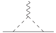
Figure 13: Triangle graph contributing to the electromagnetic form factors of the nucleon.

The “normal” threshold of the spectral function is at $t_{\rm thr}=4M_{\pi}^{2}$; however there is an anomalous threshold very close by at $t_{\rm anom}=4M_{\pi}^{2}-M_{\pi}^{4}/m_{N}^{2}$. As both coincide in the heavy-baryon limit, $t_{\rm anom}=4M_{\pi}^{2}+\mathcal{O}(M_{\pi}^{4})$, the analytic structure is distorted, as we can see comparing the contributions to the spectral function in infrared regularisation [63],

$${\rm Im}\,F_{1}^{v}(t)~{}\stackrel{{\scriptstyle{\rm IR}}}{{=}}~{}\frac{g_{A}^{2}}{192\pi F_{\pi}^{2}}(4m_{N}^{2}-M_{\pi}^{2})\left(1-\frac{4M_{\pi}^{2}}{t}\right)^{{3/2}}+\ldots~{},$$ (91)

and in HBChPT [64],

$${\rm Im}\,F_{1}^{v}(t)~{}\stackrel{{\scriptstyle{\rm HB}}}{{=}}~{}\frac{g_{A}^{2}}{96\pi F_{\pi}^{2}}(5t-8M_{\pi}^{2})\left(1-\frac{4M_{\pi}^{2}}{t}\right)^{{1/2}}+\ldots~{}.$$ (92)

While the infrared spectral function has the expected $p$-wave characteristic $\propto(1-4M_{\pi}^{2}/t)^{3/2}$, the threshold behaviour of the heavy-baryon spectral function is distorted.

Furthermore, the resummation of relativistic recoil effects in the nucleon propagator sometimes also helps to improve the phenomenological description of certain observables, as can be seen for the example of the neutron electric form factor

$$G_{E}^{n}(t)=F_{1}^{n}(t)+\frac{t}{4m_{N}^{2}}F_{2}^{n}(t)~{},$$ (93)

in Fig. 14. While convergence between leading and subleading loop order ($\mathcal{O}(p^{3})$ and $\mathcal{O}(p^{4})$, respectively) in HBChPT is rather poor, it is improved in infrared regularisation and, in addition, much closer to the data.

Figure 14: Neutron electric form factor at third and fourth order, in HBChPT and infrared regularisation, as a function of $Q^{2}=-t$. Figure taken from [63].

5.6 Quark mass dependence of the nucleon mass

As a further application of ChPT for nucleons, let us consider the quark mass expansion of the nucleon mass up to $\mathcal{O}(p^{3})$. The result is

$$m_{N}=m-{4c_{1}M_{\pi}^{2}}-{\frac{3g_{A}^{2}M_{\pi}^{3}}{32\pi F_{\pi}^{2}}}+\mathcal{O}(M_{\pi}^{4})~{}.$$ (94)

The pion loop graph Fig. 11 yields a non-analytic term $\propto M_{\pi}^{3}\propto\hat{m}^{3/2}$, but the leading correction term comes from a counterterm in $\mathcal{L}_{\pi N}^{(2)}=c_{1}\bar{\psi}\langle\chi_{+}\rangle\psi+\ldots\,$, with an unknown low-energy constant $c_{1}$. $c_{1}$ is closely related to the so-called $\pi N$ $\sigma$-term. We define the scalar form factor of the nucleon according to

$$\langle N(p^{\prime})|\hat{m}(\bar{u}u+\bar{d}d)|N(p)\rangle=\sigma(t)\bar{u}(p^{\prime})u(p)~{},\quad t=(p-p^{\prime})^{2}~{}.$$ (95)

The $\sigma$-term is then given by

$$\sigma\equiv\sigma(0)=\frac{\hat{m}}{2m_{N}}\langle N|\bar{u}u+\bar{d}d|N\rangle~{}.$$ (96)

$\sigma$ to $\mathcal{O}(p^{3})$ can be calculated from (94) using the Feynman–Hellman theorem,

$$\sigma=\hat{m}\dfrac{\partial m_{N}}{\partial\hat{m}}=-{4c_{1}M_{\pi}^{2}}-{\dfrac{9g_{A}^{2}M_{\pi}^{4}}{32\pi F_{\pi}^{2}}}+\mathcal{O}(M_{\pi}^{4})~{},$$ (97)

so is is indeed given by $c_{1}$ at leading order. Furthermore, $\sigma$ is related to the interesting question: how much do strange quarks contribute to nucleon properties? In this case, we consider the strangeness contribution to $m_{N}$, which is related to $\sigma$ by

$$\sigma=\frac{\hat{m}}{2m_{N}}\frac{\langle N|\bar{u}u+\bar{d}d-2\bar{s}s|N\rangle}{1-{y}}~{},\quad y=\frac{2\langle N|\bar{s}s|N\rangle}{\langle N|\bar{u}u+\bar{d}d|N\rangle}~{}.$$ (98)

Now $(m_{s}-\hat{m})(\bar{u}u+\bar{d}d-2\bar{s}s)$ is the part of $\mathcal{L}_{\rm QCD}$ that produces the SU(3) mass splittings and can therefore be related to differences in the baryon octet masses,

$$\sigma=\frac{{\hat{\sigma}}}{1-{y}}~{},\quad\hat{\sigma}=\frac{\hat{m}}{m_{s}-\hat{m}}\bigl{(}m_{\Xi}+m_{\Sigma}-2m_{N}\bigr{)}\simeq 26~{}{\rm MeV}~{}.$$ (99)

Higher-order corrections lead to a modified value $\hat{\sigma}\to(36\pm 7)$ MeV [65] (see also references therein for background, e.g. [66, 67]). But we conclude that, if we know $\sigma$, we know $y$ and can therefore deduce information on the strangeness content of the nucleon.

We remember that we learnt about the quark mass dependence of $M_{\pi}^{2}$ from $\pi\pi$ scattering; it turns out that, here again, the quark mass dependence of $m_{N}$ and the $\sigma$-term are closely related to $\pi N$ scattering. $\pi N$ scattering amplitudes can be separated into isospin even and odd parts,

$$T_{\pi N}^{\pm}=\frac{1}{2}\bigl{[}T(\pi^{-}p\to\pi^{-}p)\pm T(\pi^{+}p\to\pi^{+}p)\bigr{]}~{},$$ (100)

and we can decompose $T^{\pm}$ further into spin flip/non-flip amplitudes. Without going into all the details, let us consider the specific combinations $\bar{D}^{\pm}$ of $\pi N$ amplitudes. In ChPT, the following relation can be proven:

$$\Sigma\equiv F_{\pi}^{2}\bar{D}^{+}\bigl{(}s=u=m_{N}^{2},t=2M_{\pi}^{2}\bigr{)}=\sigma(2M_{\pi}^{2})+\Delta_{R}~{}.$$ (101)

The specific kinematic point $s=u=m_{N}^{2},\,t=2M_{\pi}^{2}$ at which $\bar{D}^{+}$ is to be evaluated is known as the Cheng–Dashen point.

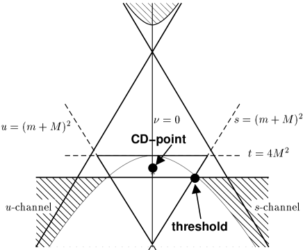
Figure 15: Mandelstam plane for $\pi N$ scattering, with the position of the $s$-channel threshold and the Cheng–Dashen (CD) point. The figure is a modified version of one taken from [68].

As shown in Fig. 15, it lies in the unphysical region (which is, in the $s$-channel, limited by $s\geq(m_{N}+M_{\pi})^{2}$, $t\leq 0$). The remainder $\Delta_{R}=\mathcal{O}(M_{\pi}^{4})$ in (101) is very small, $\Delta_{R}\lesssim 2$ MeV [69].

The procedure to learn about the strangeness content of the nucleon therefore consists of the following steps: (1) from $\pi N$ scattering, deduce the amplitude $\bar{D}^{+}$ at the Cheng–Dashen point; (2) use (101) to calculate $\sigma(2M_{\pi}^{2})$; (3) extrapolate $\sigma(t)$ to $t=0$; (4) calculate $y$ from $\sigma$ using (99).

Step (1), the extrapolation into the unphysical region, is done using dispersion relations, with the result

$$\Sigma=60\pm 7~{}{\rm MeV}~{}.$$ (102)

Step (2) is then safe due to the smallness of $\Delta_{R}$. The crucial part is step (3),

$$\sigma(2M_{\pi}^{2})=\sigma(0)+\Delta\sigma~{},$$ (103)

i.e. we have to understand the $t$-dependence of the scalar form factor $\sigma(t)$. A crude estimate would be to linearise the form factor,

$$\sigma(t)=\sigma(0)\Bigl{\{}1+\dfrac{1}{6}{\langle r^{2}\rangle_{\sigma}}\,t+\ldots\Bigr{\}}~{},$$ (104)

and assume $\langle r^{2}\rangle_{\sigma}\simeq\langle r^{2}\rangle_{\rm EM}=0.8~{}{\rm fm}^{2}$, leading to $\Delta\sigma\approx 3.5~{}{\rm MeV}$. A complete one-loop calculation yields a value not too far from this, $\Delta\sigma=4.6$ MeV. We would deduce $\sigma\approx 55~{}{\rm MeV}$ and, consequently,

$$y=1-\dfrac{\hat{\sigma}}{\sigma}=1-\dfrac{35~{}{\rm MeV}}{55~{}{\rm MeV}}\approx 0.4~{},$$ (105)

which appears far bigger than what one would naively expect. This was for some time known as the “$\sigma$-term puzzle”: are 300 MeV of nucleon mass due to strange quarks?

The resolution lies in step (3), when one considers the scalar form factor beyond one loop, see Fig. 16: it involves isoscalar $s$-wave $\pi\pi$ rescattering, which we found earlier to be strong (see Sect. 4.9).

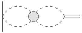
Figure 16: The scalar form factor of the nucleon beyond one loop. Full, dashed, and double lines denote nucleons, pions, and the scalar source, respectively.

A dispersive analysis yields $\langle r^{2}\rangle_{\sigma}\approx 2\langle r^{2}\rangle_{EM}$ and a large curvature term, with the result $\Delta\sigma\approx 15~{}{\rm MeV}$ [70]. The $\sigma$-term is then much smaller,

$$\sigma\approx 45~{}{\rm MeV}~{},\vspace{-1mm}$$ (106)

we now find $y\approx 0.2$ and a sizeable, but not outrageously large strangeness contribution to the nucleon mass,

$$\langle N|m_{s}\bar{s}s|N\rangle\simeq 130~{}{\rm MeV}~{}.$$ (107)

5.7 $\pi N$ scattering lengths

In order to improve the knowledge of the $\sigma$-term, it would be useful to have precise information on $\pi N$ scattering in the threshold region (which is closest to the Cheng–Dashen point), or, more precisely, on the scattering lengths, defined by

$$a^{\pm}=\frac{1}{4\pi(1+M_{\pi}/m_{N})}T^{\pm}\left(s=(m_{N}+M_{\pi})^{2}\right)~{}.$$ (108)

In ChPT at leading orders, these have the following expansion [71, 72]:

$$a^{-} = \frac{{M_{\pi}}}{8\pi(1+M_{\pi}/m_{N})F_{\pi}^{2}}+\mathcal{O}\bigl{(}{M_{\pi}^{3}}\bigr{)}~{},$$

$$a^{+} = {0}+\frac{{M_{\pi}^{2}}(-g_{A}^{2}+8m_{N}(-2c_{1}+c_{2}+c_{3}))}{16\pi m_{N}(1+M_{\pi}/m_{N})F_{\pi}^{2}}+\mathcal{O}\bigl{(}{M_{\pi}^{3}}\bigr{)}~{}.\vspace{-1mm}$$ (109)

Numerically we have $a^{-}=8.0\times 10^{-2}M_{\pi}^{-1}$ plus small higher-order corrections. In contrast, $a^{+}$ vanishes at leading order $p^{1}$, receives contributions of several LECs at $\mathcal{O}(p^{2})$, and can be seen to converge rather badly. This means that precisely the isoscalar scattering length that would be helpful in constraining the $\sigma$-term is barely known from ChPT.

Precise experimental information on the scattering lengths can be obtained from pionic hydrogen and pionic deuterium measurements, in analogy to the discussion of pionium lifetime for the $\pi\pi$ scattering lengths. The best values deduced thereof [73] (see also experimental references therein) are given by

$$a^{-}=(8.52\pm 0.18)\times 10^{-2}M_{\pi}^{-1}~{},\quad a^{+}=(0.15\pm 0.22)\times 10^{-2}M_{\pi}^{-1}~{}.\vspace{-1mm}$$ (110)

$a^{+}$ is seen to be very small, and quite sensitive to isospin breaking corrections.

6 Outlook

Instead of a summary, we rather give an outlook on various aspects of ChPT that, due to lack of time and space, could not be covered in these lectures.

In the Goldstone boson sector, of course there are many more processes of high physical interest, e.g. various meson decays, further scattering problems etc. The whole sector of odd intrinsic parity (“chiral anomaly”, Wess–Zumino–Witten term [14]) has not been touched upon, although it is responsible for such fundamental decays as $\pi^{0}\to\gamma\gamma$ or $\eta\to\gamma\gamma$. A whole new set of Lagrangian terms is furthermore needed for weak matrix elements, e.g. for non-leptonic kaon decays. We have only in passing hinted at the links to dispersion theory, and relations of the chiral phenomenology to large-$N_{c}$ arguments have been completely ignored.

In the single-baryon sector, some of the most noteworthy omissions include the highly interesting topic of isospin violation in $\pi N$ scattering; the analysis of pion photo-/electroproduction $\gamma^{(*)}N\to\pi N$, which has proven to be one of the key successes in the development of baryon ChPT (see [74] and references therein); Compton scattering $\gamma N\to\gamma N$ and nucleon polarisabilities. An important extension of ChPT with baryons is the inclusion of explicit spin-3/2 ($\Delta$) degrees of freedom (“small-scale expansion” [75]).

The topic of two-and-more-nucleon systems has been covered in the lectures by Chen, Hanhart [76], and Machleidt at this workshop. The connections to lattice QCD, which are another major point of research at present, concerning chiral extrapolations, ChPT in a finite volume and at non-zero lattice spacing, (partially) quenched ChPT have been touched upon in the lectures by Chen.

Acknowledgements

I would like to thank the organisers of “Physics and Astrophysics of Hadrons and Hadronic Matter” for a wonderful workshop, and in particular for their overwhelming hospitality during the week in Shantiniketan. I am grateful to Jürg Gasser and Ulf-G. Meißner for useful comments on the manuscript. This work was supported in parts by the DFG (SFB/TR 16) and the EU I3HP Project (RII3-CT-2004-506078).

References

- [1] G. Ecker, Prog. Part. Nucl. Phys. 35 (1995) 1.
- [2] A. V. Manohar, arXiv:hep-ph/9606222.
- [3] U.-G. Meißner, arXiv:hep-ph/9711365.
- [4] S. Scherer, Adv. Nucl. Phys. 27 (2003) 277.
- [5] J. Gasser, Lect. Notes Phys. 629 (2004) 1.
- [6] G. Colangelo, http://ltpth.web.psi.ch/zuoz2006.
- [7] V. Bernard, U.-G. Meißner, arXiv:hep-ph/0611231.
- [8] W. Heisenberg, H. Euler, Z. Phys. 98 (1936) 714.
- [9] S. Weinberg, Physica A 96 (1979) 327.
- [10] S. Schael et al. [ALEPH Collaboration], Phys. Rept. 421 (2005) 191.
- [11] C. Vafa, E. Witten, Nucl. Phys. B 234 (1984) 173.
- [12] S. R. Coleman, J. Wess, B. Zumino, Phys. Rev. 177 (1969) 2239; C. G. Callan, S. R. Coleman, J. Wess, B. Zumino, Phys. Rev. 177 (1969) 2247.
- [13] H. Leutwyler, Annals Phys. 235 (1994) 165.
- [14] J. Wess, B. Zumino, Phys. Lett. B 37 (1971) 95; E. Witten, Nucl. Phys. B 223 (1983) 422.
- [15] R. Urech, Nucl. Phys. B 433 (1995) 234.
- [16] R. F. Dashen, Phys. Rev. 183 (1969) 1245.
- [17] S. Weinberg, Phys. Rev. Lett. 17 (1966) 616.
- [18] J. Gasser, H. Leutwyler, Annals Phys. 158 (1984) 142.
- [19] J. Gasser, H. Leutwyler, Nucl. Phys. B 250 (1985) 465.
- [20] J. Bijnens, G. Colangelo, G. Ecker, JHEP 9902 (1999) 020.
- [21] G. Ecker, J. Gasser, H. Leutwyler, A. Pich, E. de Rafael, Phys. Lett. B 223 (1989) 425.
- [22] G. Ecker, J. Gasser, A. Pich, E. de Rafael, Nucl. Phys. B 321 (1989) 311.
- [23] J. F. Donoghue, C. Ramirez, G. Valencia, Phys. Rev. D 39 (1989) 1947.
- [24] J. Bijnens, G. Colangelo, G. Ecker, Annals Phys. 280 (2000) 100.
- [25] M. Knecht, B. Moussallam, J. Stern, N. H. Fuchs, Nucl. Phys. B 457 (1995) 513.
- [26] J. Bijnens, G. Colangelo, G. Ecker, J. Gasser, M. E. Sainio, Nucl. Phys. B 508 (1997) 263 [Erratum-ibid. B 517 (1998) 639].
- [27] S. Pislak et al., Phys. Rev. D 67 (2003) 072004.
- [28] L. Masetti, arXiv:hep-ex/0610071.
- [29] J. R. Batley et al. [NA48/2 Collaboration], Phys. Lett. B 633 (2006) 173.
- [30] B. Adeva et al. [DIRAC Collaboration], Phys. Lett. B 619 (2005) 50.
- [31] V. Bernard, N. Kaiser, U.-G. Meißner, Nucl. Phys. B 457 (1995) 147.
- [32] K. M. Watson, Phys. Rev. 88 (1952) 1163.
- [33] A. Pais, S. B. Treiman, Phys. Rev. 168 (1968) 1858.
- [34] U.-G. Meißner, G. Müller, S. Steininger, Phys. Lett. B 406 (1997) 154 [Erratum-ibid. B 407 (1997) 454].
- [35] N. Cabibbo, Phys. Rev. Lett. 93 (2004) 121801; N. Cabibbo, G. Isidori, JHEP 0503 (2005) 021.
- [36] G. Colangelo, J. Gasser, B. Kubis, A. Rusetsky, Phys. Lett. B 638 (2006) 187.
- [37] E. Gamiz, J. Prades, I. Scimemi, arXiv:hep-ph/0602023.
- [38] S. Deser, M. L. Goldberger, K. Baumann, W. E. Thirring, Phys. Rev. 96 (1954) 774.
- [39] A. Gall, J. Gasser, V. E. Lyubovitskij, A. Rusetsky, Phys. Lett. B 462 (1999) 335.
- [40] J. Gasser, V. E. Lyubovitskij, A. Rusetsky, Phys. Lett. B 471 (1999) 244.
- [41] H. Sazdjian, Phys. Lett. B 490 (2000) 203.
- [42] J. Gasser, V. E. Lyubovitskij, A. Rusetsky, A. Gall, Phys. Rev. D 64 (2001) 016008.
- [43] H. Leutwyler, arXiv:hep-ph/0612112.
- [44] Ph. Boucaud et al. [ETM Collaboration], arXiv:hep-lat/0701012.
- [45] G. Colangelo, J. Gasser, H. Leutwyler, Phys. Rev. Lett. 86 (2001) 5008.
- [46] H. Leutwyler, Phys. Lett. B 378 (1996) 313.
- [47] A. Duncan, E. Eichten, H. Thacker, Phys. Rev. Lett. 76 (1996) 3894; J. Bijnens, J. Prades, Nucl. Phys. B 490 (1997) 239; J. F. Donoghue, A. F. Perez, Phys. Rev. D 55 (1997) 7075; B. Ananthanarayan, B. Moussallam, JHEP 0406 (2004) 047.
- [48] D. G. Sutherland, Phys. Lett. 23 (1966) 384.
- [49] R. Baur, J. Kambor, D. Wyler, Nucl. Phys. B 460 (1996) 127.
- [50] J. Gasser, H. Leutwyler, Nucl. Phys. B 250 (1985) 539.
- [51] H. H. Adam et al. [WASA-at-COSY Collaboration], arXiv:nucl-ex/ 0411038; S. Giovannella et al. [KLOE Collaboration], arXiv:hep-ex/ 0505074; A. Starostin, Acta Phys. Slov. 56 (2005) 345.
- [52] J. Kambor, C. Wiesendanger, D. Wyler, Nucl. Phys. B 465 (1996) 215.
- [53] B. V. Martemyanov, V. S. Sopov, Phys. Rev. D 71 (2005) 017501.
- [54] B. Borasoy, R. Nißler, Eur. Phys. J. A 26 (2005) 383.
- [55] J. Gasser, H. Leutwyler, Phys. Rept. 87 (1982) 77.
- [56] J. Gasser, M. E. Sainio, A. Švarc, Nucl. Phys. B 307 (1988) 779.
- [57] E. Jenkins, A. V. Manohar, Phys. Lett. B 255 (1991) 558.
- [58] V. Bernard, N. Kaiser, J. Kambor, U.-G. Meißner, Nucl. Phys. B 388 (1992) 315.
- [59] T. Becher, H. Leutwyler, Eur. Phys. J. C 9 (1999) 643.
- [60] P. J. Ellis, H. B. Tang, Phys. Rev. C 57 (1998) 3356.
- [61] J. L. Goity, D. Lehmann, G. Prézeau, J. Saez, Phys. Lett. B 504 (2001) 21; D. Lehmann, G. Prézeau, Phys. Rev. D 65 (2002) 016001.
- [62] M. R. Schindler, J. Gegelia, S. Scherer, Phys. Lett. B 586 (2004) 258.
- [63] B. Kubis, U.-G. Meißner, Nucl. Phys. A 679 (2001) 698.
- [64] V. Bernard, N. Kaiser, U.-G. Meißner, Nucl. Phys. A 611 (1996) 429.
- [65] B. Borasoy, U.-G. Meißner, Annals Phys. 254 (1997) 192.
- [66] J. Gasser, Annals Phys. 136 (1981) 62.
- [67] V. Bernard, N. Kaiser, U.-G. Meißner, Z. Phys. C 60 (1993) 111.
- [68] P. Büttiker, U.-G. Meißner, Nucl. Phys. A 668 (2000) 97.
- [69] V. Bernard, N. Kaiser, U.-G. Meißner, Phys. Lett. B 389 (1996) 144.
- [70] J. Gasser, H. Leutwyler, M. E. Sainio, Phys. Lett. B 253 (1991) 260.
- [71] V. Bernard, N. Kaiser, U.-G. Meißner, Phys. Lett. B 309 (1993) 421.
- [72] N. Fettes, U.-G. Meißner, Nucl. Phys. A 676 (2000) 311.
- [73] U.-G. Meißner, U. Raha, A. Rusetsky, Phys. Lett. B 639 (2006) 478.
- [74] V. Bernard, N. Kaiser, U.-G. Meißner, Int. J. Mod. Phys. E 4 (1995) 193.
- [75] T. R. Hemmert, B. R. Holstein, J. Kambor, J. Phys. G 24 (1998) 1831.
- [76] C. Hanhart, arXiv:nucl-th/0703028.