QCD corrections to tri-boson production

Abstract

We present a computation of the next-to-leading order QCD corrections to the production of three $Z$ bosons at the LHC. We calculate these corrections using a completely numerical method that combines sector decomposition to extract infrared singularities with contour deformation of the Feynman parameter integrals to avoid internal loop thresholds. The NLO QCD corrections to $pp\to ZZZ$ are approximately 50%, and are badly underestimated by the leading order scale dependence. However, the kinematic dependence of the corrections is minimal in phase space regions accessible at leading order.

I Introduction

The search for and interpretation of new physics at the LHC will require a precise understanding of the Standard Model. Without accurate QCD predictions and reliable error estimates for important observables, mistakes in interpreting experimental results may occur. Notable recent examples where poor theoretical understanding has hindered the analysis of an experimental result are the deviation of the Brookhaven muon $g-2$ measurement from the Standard Model prediction, the excess of bottom quark production in Run I of the Tevatron, and the discrepancy in the weak mixing angle obtained by NuTeV. At the LHC, all analyses require perturbative calculations to at least next-to-leading order (NLO) in $\alpha_{s}$, the QCD coupling constant, in order to make quantitative predictions that are free from debilitating theoretical uncertainties. This need for higher order calculations at the LHC has been summarized in an experimental ”NLO wishlist” of processes for which QCD corrections are desired NLOwish .

A cross section at higher orders in perturbation theory consists of two primary components: virtual corrections, in which additional loops are added to the Born-level matrix element, and real corrections, in which additional partons are radiated. Each contribution is separately infrared divergent. They must be combined and summed over degenerate final states to obtain a finite result. Initial-state collinear singularities must be absorbed into the definitions of the parton distribution functions.

Well-developed techniques exist for the calculation of real emission corrections at NLO. However, the calculation of virtual corrections to processes with many particles in the final state remains a challenge. For this reason, our primary focus in this paper will be to develop an approach to computing virtual corrections to $2\to 3$ scattering processes. We begin by discussing methods currently used to perform such calculations. Well-developed techniques exist for calculating one-loop virtual corrections to $2\to 2$ and simpler processes. The matrix elements are obtained via a standard Feynman diagram calculation. The tensor integrals are reduced to a basis of scalar integrals via a reduction algorithm such as Passarino-Veltman Passarino:1978jh . The basis integrals are then computed analytically using a Feynman parameter representation, with care being taken to extract all infrared singularities that occur in the parametric integration. These integrals are typically performed with Euclidean kinematics; after the analytic expression is derived, the resulting logarithms and polylogarithms are analytically continued to the Minkowski region.

Several problems arise when this approach is extended to $2\to 3$ and more complicated scattering processes. The increase in algebraic complexity alone makes the procedure difficult. The singularity extraction and analytic continuation to the physical region are typically done on a case-by-case basis for each scattering process; the large number of processes for which NLO QCD computations are desired implies that studying each separately will be an enormously time-consuming task. Furthermore, the standard reduction algorithms introduce inverse Gram determinants multiplying the basis integrals; these coefficients vanish when the final-state momenta become linearly dependent, and can become arbitrarily small nearby. Although these spurious singularities cancel when all basis integrals are combined, it is difficult to establish this analytically, and they usually cause serious numerical complications. Careful studies of the boundaries and extrapolations of numerical results from safe phase space regions are typically required to obtain stable answers NLOexamples .

Because of these complications, the computation of the NLO QCD corrections to $2\to n,n\geq 3$ scattering processes is a difficult and intricate task that typically requires one year or more of effort for every interaction considered. These difficulties and the importance of these calculations to the LHC physics program have stimulated significant effort to develop new approaches for perturbative QCD computations. These include new analytic NLOan and semi-numerical NLOnum methods for evaluating loop integrals. Phenomenological results obtained with these methods include the NLO QCD corrections to $H+2~{}{\rm jets}$ Campbell:2006xx and $t\bar{t}+{\rm jet}$ Dittmaier:2007wz at the LHC, and also the matrix elements used for $W,Z+{\rm jets}$ zvi .

Ideally, an algorithm for NLO QCD calculations would be highly automated and would handle a large number of processes without the need to consider special cases. This would allow a large swath of desired corrections to be computed by a single program running in parallel on many machines. Any such approach must confront three main issues: spurious phase space singularities that appear during the reduction of tensor integrals, the extraction of soft and collinear singularities, and the presence of internal thresholds where analytic continuation is required. An approach that addresses the first two issues exists, called sector decomposition Hepp:1966eg ; Roth:1996pd ; Binoth:2000ps . It permits a completely automated, numerical extraction of infrared singularities from loop integrals. The application of this approach to an integral results in a Laurent series in $\epsilon$, the parameter of dimensional regularization, with coefficients that can be numerically integrated over Feynman parameters. Since the infrared singularity structure of a loop diagram in parametric space is completely determined by its denominator, no Passarino-Veltman reduction of tensor integrals is needed. Consequently, inverse Gram determinants never appear. The basic scalar integral which characterizes a diagram is identified and sector decomposed. The tensors become polynomials in the Feynman parameters after integration over the loop momenta; they can be treated numerically.

The remaining issue is the internal threshold structure present in loop diagrams. Thresholds occur when the internal propagators go on-shell, and a unitarity cut of the diagram leads to a physical scattering process. In Feynman parameter space, the denominator vanishes at these points, and is regulated only by the $-i0$ prescription for loop integrals. For $N$-point functions, this leads to denominators with the behavior $1/(-i0)^{N-2}$ at threshold locations. This is completely unsuitable for numerical implementation. An approach for handling thresholds in loop diagrams numerically was developed in Soper ; Soper2 . It entails a contour deformation of the Feynman parametric integrals off the real axis and into the complex plane to avoid internal thresholds. The integrals are then computed numerically. The choice of the deformation for a given diagram is easily automated.

It appears to us that the combination of sector decomposition and contour deformation provides a framework in which numerical calculations of NLO virtual corrections can be fully automated. A similar attitude was espoused in Binoth:2005ff . Our goal in this paper is to test this idea on a realistic $2\to 3$ scattering process at the LHC. We study the NLO QCD corrections to $pp\to ZZZ+X$, which acts as a background to supersymmetric tri-lepton production and appears on the NLO wishlist in NLOwish . We find that the combination of these procedures does indeed appear to be a convenient approach to NLO QCD computations.

This paper is organized as follows. In Section II we define our notation and present $pp\to ZZZ$ at leading order in QCD. In Section III we discuss our computation of the NLO QCD corrections. In particular, we present the algorithm we use for the computation of the virtual corrections. In Section IV we provide numerical results for $pp\to ZZZ+X$ at the LHC. We conclude in Section V.

II Setup and leading order process

We consider the production of three $Z$-bosons in proton-proton collisions,

$$p(P_{1})+p(P_{2})\to Z(p_{3})+Z(p_{4})+Z(p_{5})+X.$$ (1)

Within the framework of QCD factorization, the cross section for this process is

$${\rm d}\sigma=\sum_{ij}\int_{0}^{1}dx_{1}dx_{2}f_{i}^{p_{1}}(x_{1})f_{j}^{p_{2}}(x_{2}){\rm d}\sigma_{ij\to 3Z+X}(x_{1},x_{2}),$$ (2)

where the $f_{i}^{p_{j}}$ are parton distribution functions that describe the probability to find a parton $i$ with momentum $xP_{j}$ in the proton $p_{j}$. The partonic cross sections ${\rm d}\sigma_{ij}$ are computed perturbatively as an expansion in the strong coupling constant $\alpha_{s}$:

$${\rm d}\sigma_{ij}={\rm d}\sigma^{(0)}_{ij}+\left(\frac{\alpha_{s}}{\pi}\right){\rm d}\sigma^{(1)}_{ij}+{\cal O}(\alpha_{s}^{2}).$$ (3)

At leading order in this expansion, only the partonic channel $q(p_{1})+\bar{q}(p_{2})\to Z(p_{3})+Z(p_{4})+Z(p_{5})$ contributes. A representative diagram for this process is shown in Fig. (1). There are six such diagrams, which can be obtained via permutation of the final-state bosons. We neglect diagrams containing the exchange of a Higgs boson. For Higgs boson masses below $2M_{Z}$, the contributions from these diagrams are small. At next-to-leading order, both virtual corrections and additional radiative processes occur; we discuss the calculation of these components in later sections. After combining the virtual and real corrections, the partonic cross sections in Eq. (3) contain collinear singularities arising from initial-state radiation. These are absorbed into the definitions of the parton distribution functions, as discussed in a later section.

Figure 1: Representative Born-level diagram for $q\bar{q}\to ZZZ$.

The expression for the leading order cross section is

$${\rm d}\sigma^{(0)}_{q\bar{q}}=\frac{1}{4}\frac{1}{9}\frac{1}{6}\frac{1}{2\hat{s}}|{\cal M}^{(0)}|^{2}{\rm d}\Omega_{3Z},$$ (4)

where the factors $\frac{1}{4}$, $\frac{1}{9}$, and $\frac{1}{6}$ are from spin-averaging, color-averaging, and identical particles, $\hat{s}=x_{1}x_{2}s$ is the partonic center-of-momentum energy squared, $s=2P_{1}\cdot P_{2}$ is the total energy squared of the proton-proton collision and $\Omega_{3Z}$ denotes the final-state phase space. The matrix elements $|{\cal M}^{(0)}|^{2}$ have the expansion

$$|{\cal M}^{(0)}|^{2}=|{\cal M}_{0}^{(0)}|^{2}+\epsilon|{\cal M}_{1}^{(0)}|^{2},$$ (5)

where $d=4-2\epsilon$ is the space-time dimensionality in dimensional regularization. The matrix elements are simple to calculate using standard Feynman diagram techniques. We use a combination of the programs QGRAF Nogueira:1991ex , FORM Vermaseren:2000nd , and MAPLE to obtain them. The required electroweak vertex is

$$Z\bar{q}{q}: i\sqrt{\frac{8M_{W}^{2}G_{F}}{\sqrt{2}c_{w}}}\left(g_{v}+g_{a}\gamma_{5}\right),$$ (6)

$$g_{v}=\frac{T_{3}^{q}}{2}-Q_{q}s_{w}^{2},\,\,\,g_{a}=-\frac{T_{3}^{q}}{2}.$$

Here, $s_{w}^{2}=1-M_{W}^{2}/M_{Z}^{2}$ is the sine squared of the electroweak mixing angle, $T_{3}^{q}$ is the weak isospin of the quark $q$, $Q_{q}$ is the electric charge of the quark $q$ in units of the proton charge, and $G_{F}$ is the Fermi constant. Decomposing the matrix elements using the expansion in Eq. (5), the leading order cross section takes the form

$${\rm d}\sigma^{(0)}={\rm d}\sigma_{0}^{(0)}+\epsilon{\rm d}\sigma_{1}^{(0)}.$$ (7)

The ${\cal O}(\epsilon)$ term in Eq. (7) is needed in the computation of the collinear counterterms.

III Next-to-leading order corrections

The ${\cal O}(\alpha_{s})$ NLO QCD corrections consist of the following components:

1. the radiative processes $q\bar{q}\to ZZZg$, $qg\to ZZZq$, and $\bar{q}g\to ZZZ\bar{q}$;

2. the collinear counterterms which absorb the initial-state collinear singularities of these radiative processes into the parton distribution functions;

3. the one-loop virtual contributions to the leading order partonic process $q\bar{q}\to ZZZ$.

We discuss the calculation of each component in the following sections, and describe in detail the method used to compute the virtual corrections.

III.1 Real radiation

We begin with a discussion of the real radiation processes. We present in detail the process $q\bar{q}\to ZZZg$, and then note the modifications required when $qg\to ZZZq$ and $\bar{q}g\to ZZZ\bar{q}$ are considered.

Twenty-four Feynman diagrams contribute to $q(p_{1})+\bar{q}(p_{2})\to Z(p_{3})+Z(p_{4})+Z(p_{5})+g(p_{g})$. A few representative samples are shown in Fig. (2). Collinear and soft singularities occur when the gluon is emitted from an initial fermion line, indicating that the Laurent series for this process begins at $1/\epsilon^{2}$. The expression for the cross section is

$${\rm d}\sigma^{(1)}_{q\bar{q}\to 3Z+g}=\frac{1}{4}\frac{1}{9}\frac{1}{6}\frac{1}{2\hat{s}}|{\cal M}_{3Z+g}^{(1)}|^{2}{\rm d}\Omega_{3Z+g}.$$ (8)

The matrix elements are again simple to obtain using standard techniques.

Figure 2: Representative diagrams contributing to $q\bar{q}\to ZZZg$.

To discuss the extraction of the infrared singularities, it is convenient to introduce an explicit parameterization of the final-state phase space. In terms of the partonic momenta, the phase space takes the form

$$\int{\rm d}\Omega_{3Z+g} = \int\frac{d^{4}p_{3}}{(2\pi)^{3}}\frac{d^{4}p_{4}}{(2\pi)^{3}}\frac{d^{4}p_{5}}{(2\pi)^{3}}\frac{d^{d}p_{g}}{(2\pi)^{d-1}}\,\delta(p_{3}^{2}-M_{Z}^{2})\,\delta(p_{4}^{2}-M_{Z}^{2})\,\delta(p_{5}^{2}-M_{Z}^{2})\,\delta(p_{g}^{2})$$ (9)

$$\times (2\pi)^{d}\delta^{(d)}(p_{1}+p_{2}-p_{3}-p_{4}-p_{5}-p_{g}).$$

Since there are no singularities associated with the $3Z$ phase space, we evaluate it directly in four dimensions. We now partition the phase space using

$$\int\frac{d^{4}p_{3}}{(2\pi)^{3}}\frac{d^{4}p_{4}}{(2\pi)^{3}}\frac{d^{4}p_{5}}{(2\pi)^{3}}\frac{d^{d}p_{g}}{(2\pi)^{d-1}}\,\delta(p_{3}^{2}-M_{Z}^{2})\,\delta(p_{4}^{2}-M_{Z}^{2})\,\delta(p_{5}^{2}-M_{Z}^{2})\,\delta(p_{g}^{2})$$ (10)

$$\times (2\pi)^{d}\delta^{(d)}(p_{1}+p_{2}-p_{3}-p_{4}-p_{5}-p_{g})=\int\frac{ds_{345}}{2\pi}\int\frac{d^{d}p_{345}}{(2\pi)^{d-1}}\frac{d^{d}p_{g}}{(2\pi)^{d-1}}\,\delta(p_{345}^{2}-s_{345})\,\delta(p_{g}^{2})$$

$$\times (2\pi)^{d}\delta^{(d)}(p_{1}+p_{2}-p_{345}-p_{g})\int{\rm d}\Omega_{3Z}(p_{345}),$$

where $\Omega_{3Z}(p_{345})$ denotes the $3Z$ phase space with the sum of the three boson momenta giving $p_{345}$ rather than $p_{1}+p_{2}$. We evaluate the gluon phase space in the partonic center-of-momentum frame by introducing the explicit four-momenta

$$p_{1}=\frac{\sqrt{\hat{s}}}{2}\left(1,0,0,1\right),\,\,p_{2}=\frac{\sqrt{\hat{s}}}{2}\left(1,0,0,-1\right),\,\,p_{g}=E_{g}\left(1,0,s_{g},c_{g}\right).$$ (11)

We use the $\delta$-functions to remove as many integrations as possible, and change variables in those remaining so that the boundaries are at 0 and 1. We arrive at the following expression for the phase space:

$$\int{\rm d}\Omega_{3Z+g}=\frac{\pi^{1-\epsilon}}{2(2\pi)^{d-1}\Gamma(1-\epsilon)}\int_{0}^{1}d\lambda_{1}d\lambda_{5}\left[\lambda_{1}(1-\lambda_{1})\right]^{-\epsilon}\lambda_{5}^{1-2\epsilon}\left(1-9z^{2}\right)^{2-2\epsilon}\int{\rm d}\Omega_{3Z}(p_{345}).$$ (12)

Here, $z^{2}=M_{Z}^{2}/\hat{s}$, and the expressions for the invariant masses in terms of the hypercube variables $\lambda_{1}$ and $\lambda_{5}$ are

$$s_{345} = (p_{3}+p_{4}+p_{5})^{2}=(1-9z^{2})(1-\lambda_{5})+9z^{2},$$

$$s_{1g} = (p_{1}-p_{g})^{2}=-\lambda_{5}(1-\lambda_{1})(1-9z^{2}),$$

$$s_{2g} = (p_{2}-p_{g})^{2}=-\lambda_{5}\lambda_{1}(1-9z^{2}).$$ (13)

In writing these expressions we have set the overall energy scale $\hat{s}=1$; it can be restored at the end using dimensional analysis.

The singular terms in the matrix elements come from the following three sources.

1. Interferences between diagrams where the gluon is emitted from the quark line with momentum $p_{1}$. When the denominator of the off-shell quark propagator $s_{1g}$ in Eq. (13) is combined with the phase space in Eq. (12), the singular structure $\lambda_{5}^{-1-2\epsilon}(1-\lambda_{1})^{-1-\epsilon}$ is obtained.

2. Interferences between diagrams where the gluon is emitted from the anti-quark line with momentum $p_{2}$: these lead to the singular structure $\lambda_{5}^{-1-2\epsilon}\lambda_{1}^{-1-\epsilon}$.

3. Interferences containing the denominator $1/s_{1g}/s_{2g}$: if care is taken to sum over only physical gluon polarizations in the final state, these contain only the soft singularity $\lambda_{5}^{-1-2\epsilon}$.

To extract the singularities as a Laurent series in $\epsilon$, we use the following standard plus distribution expansion:

$$\lambda^{-1+\epsilon}=\frac{1}{\epsilon}\delta(\lambda)+\sum_{n=0}\frac{\epsilon^{n}}{n!}\left[\frac{{\rm ln}^{n}\lambda}{\lambda}\right]_{+},$$ (14)

where the plus distributions are defined via

$$\int_{0}^{1}d\lambda\left[\frac{f(\lambda)}{\lambda}\right]_{+}g(\lambda)=\int_{0}^{1}d\lambda\frac{f(\lambda)}{\lambda}\left(g(\lambda)-g(0)\right).$$ (15)

After using these expansions, the cross section for $q\bar{q}\to ZZZg$ takes the form

$${\rm d}\sigma^{(1)}_{q\bar{q}\to 3Z+g}=\frac{{\cal A}_{2}}{\epsilon^{2}}+\frac{{\cal A}_{1}}{\epsilon}+{\cal A}_{0}.$$ (16)

The ${\cal A}_{i}$ are integrable, $\epsilon$-independent quantities that contain the complete kinematic information of the final state. The $1/\epsilon^{2}$ singularities, where $\lambda_{5}\to 0$ and $\lambda_{1}\to 0$ or $1$, cancel against the virtual contributions to $q\bar{q}\to ZZZ$. The $1/\epsilon$ terms where $\lambda_{1}\to 0$ or $1$ are removed by the collinear counterterms discussed in the next section. The $1/\epsilon$ singularities where $\lambda_{5}\to 0$ cancel against a combination of the virtual corrections and collinear counterterms.

The matrix elements for the remaining real radiation processes $qg\to ZZZq$ and $\bar{q}g\to ZZZ\bar{q}$ are identical. They each consist of twenty-four diagrams. The cross section is

$${\rm d}\sigma^{(1)}_{qg\to 3Z+q}=\frac{1}{4(1-\epsilon)}\frac{1}{24}\frac{1}{6}\frac{1}{2\hat{s}}|{\cal M}_{3Z+q}^{(1)}|^{2}{\rm d}\Omega_{3Z+q},$$ (17)

where we have used the fact that the gluon has $2(1-\epsilon)$ physical polarizations in $d=4-2\epsilon$ dimensions. We extract singularities using the same phase space parameterization and expansion in plus distributions discussed above. For this process, only collinear singularities where $\lambda_{1}\to 0$ or $1$ occur. These are removed by the collinear counterterms described in the next section.

III.2 Collinear counterterms

The radiative processes discussed in the previous section contain collinear singularities that must be absorbed into the parton distribution functions. To do so, we begin by expressing the bare distribution functions and cross sections in Eq. (2) in terms of the renormalized ones,

$${\rm d}\sigma=\sum_{ij}\int_{0}^{1}dx_{1}dx_{2}\hat{f}_{i}^{p_{1}}(x_{1})\hat{f}_{j}^{p_{2}}(x_{2}){\rm d}\hat{\sigma}_{ij}(x_{1},x_{2}).$$ (18)

The renormalized parton distribution functions $\hat{f}_{i}$ are related to the bare ones $f_{i}$ via

$$\hat{f}_{i}=\Gamma_{ij}\otimes f_{j}.$$ (19)

We have introduced the convolution integral

$$(f\otimes g)(x)=\int_{0}^{1}dydzf(y)g(z)\delta(x-yz),$$ (20)

and we have implicitly summed over repeated parton indices. The functions $\Gamma_{ij}$ are given by

$$\Gamma_{ij}(x)=\delta_{ij}\delta(1-x)-\frac{\alpha_{s}}{\pi}\frac{P^{(0)}_{ij}(x)}{\epsilon}.$$ (21)

The DGLAP kernels $P^{(0)}_{ij}$ in the $\overline{\rm MS}$ scheme can be found in Ellis:1991qj ; those required here are

$$P^{(0)}_{qq}(x) = \frac{2}{3}\left\{\frac{3}{2}\delta(1-x)+\frac{2}{[1-x]_{+}}-(1+x)\right\},$$

$$P^{(0)}_{qg}(x) = \frac{1}{4}\left\{x^{2}+(1-x)^{2}\right\}.$$ (22)

To proceed, we substitute Eq. (21) into Eq. (18), equate this to Eq. (2), and solve for the renormalized cross sections ${\rm d}\hat{\sigma}_{ij}$. We expand the renormalized cross sections in the strong coupling constant

$${\rm d}\hat{\sigma}_{ij}={\rm d}\hat{\sigma}^{(0)}_{ij}+\left(\frac{\alpha_{s}}{\pi}\right){\rm d}\hat{\sigma}^{(1)}_{ij},$$ (23)

and employ Eq. (3) to obtain the following relations between the bare and renormalized cross sections at each order in $\alpha_{s}$:

$${\rm d}\hat{\sigma}^{(0)}_{q\bar{q}}(x_{1},x_{2}) = {\rm d}\sigma^{(0)}_{q\bar{q}}(x_{1},x_{2});$$

$${\rm d}\hat{\sigma}^{(1)}_{q\bar{q}}(x_{1},x_{2}) = {\rm d}\sigma^{(1)}_{q\bar{q}}+\frac{1}{\epsilon}\int_{0}^{1}dyP^{(0)}_{qq}(y)\left[{\rm d}\sigma^{(0)}_{q\bar{q}}(x_{1},x_{2}y)+{\rm d}\sigma^{(0)}_{q\bar{q}}(x_{1}y,x_{2})\right];$$

$${\rm d}\hat{\sigma}^{(1)}_{qg}(x_{1},x_{2}) = {\rm d}\sigma^{(1)}_{qg}+\frac{1}{\epsilon}\int_{0}^{1}dyP^{(0)}_{qg}(y)\,{\rm d}\sigma^{(0)}_{q\bar{q}}(x_{1},x_{2}y).$$ (24)

The collinear counterterms that must be added to the perturbatively computed cross sections are the integrals in Eq. (24). These are straightforward to compute as Laurent series in $\epsilon$, as we do for the real radiation cross sections in Eq. (16). We note that the convolution variable $y$ maps onto the invariant mass $s_{345}$ in Eq. (13). This makes it simple to check analytically that the singularities in the real radiation cross section that occur as $\lambda_{1}\to 0,1$ cancel. We also note that the ${\cal O}(\epsilon)$ term in the leading order cross section in Eq. (7) contributes to the collinear counterterms at the finite level.

III.3 Virtual corrections

Finally, the virtual corrections to the partonic process $q\bar{q}\to VVV$ must be computed. Forty-eight one-loop diagrams contribute to this process; these must be interfered with the six tree-level diagrams. A representative sample of virtual diagrams is given in Fig. (3). The expressions for the interferences are simple to obtain with standard techniques. We regulate all singularities using dimensional regularization, in which scale-less integrals are set to zero. Consequently, there are no contributions from self-energy insertions on the external legs. All singularities that remain when the one-loop diagrams are combined are infrared in origin.

Figure 3: Representative one-loop diagrams contributing to $q\bar{q}\to ZZZ$.

The treatment of the virtual corrections to $2\to 3$ processes is the main point of this paper, so we discuss this here in detail. We will use the pentagon appearing as the rightmost diagram in Fig. (3) to demonstrate our technique. We begin by neglecting all numerator algebra that appears from the Feynman rules and Dirac traces when this diagram is interfered with the tree-level diagrams, and focus on the scalar topology. The basic scalar integral for this topology is

$${\cal I}=\int\frac{d^{d}k}{(2\pi)^{d}}\frac{1}{k^{2}}\frac{1}{(k+p_{1})^{2}}\frac{1}{(k+p_{3}+p_{4}-p_{2})^{2}}\frac{1}{(k+p_{3}-p_{2})^{2}}\frac{1}{(k-p_{2})^{2}}.$$ (25)

The $+i0$ prescription associated with each denominator has been suppressed for notational ease. After introducing a standard Feynman parameter representation, this integral becomes

$${\cal I}=-\frac{i\Gamma(3+\epsilon)}{(4\pi)^{d/2}}\int_{0}^{1}\prod\limits_{i=1}^{5}dx_{i}\,\delta\left(1-\sum_{n=1}^{5}x_{i}\right)[\Delta-i0]^{-3-\epsilon},$$ (26)

where

$$\Delta = 2x_{2}(x_{3}+x_{4})\,p_{1}\cdot p_{3}+2x_{2}x_{3}\,p_{1}\cdot p_{4}+2(x_{1}+x_{2})(x_{3}+x_{4})\,p_{2}\cdot p_{3}+2x_{3}(x_{1}+x_{2})\,p_{2}\cdot p_{4}$$ (27)

$$-2x_{2}(x_{3}+x_{4}+x_{5})\,p_{1}\cdot p_{2}-2x_{3}(x_{1}+x_{2}+x_{5})p_{3}\cdot p_{4}-x_{3}(x_{1}+x_{2}+x_{4}+x_{5})\,M_{Z}^{2}$$

$$-(x_{3}+x_{4})(x_{1}+x_{2}+x_{5})\,M_{Z}^{2}.$$

We must discuss two features of this integral: the extraction of infrared singular terms and the treatment of internal thresholds.

We begin by considering the singular structure. This integral exhibits infrared singularities as various combinations of $x_{i}$ approach 0 or 1. A convenient, easily automated prescription for extracting such singularities from loop integrals was presented in Binoth:2000ps . We summarize here the salient features of this technique.

1. To remove singularities that occur as $x_{i}\to 1$, we first split the integral into primary sectors. There is a primary sector for each Feynman parameter; for example, the primary sector associated with $x_{1}$ is obtained by making the following variable changes in Eq. (26):

   $$x_{j}=x_{1}x^{{}^{\prime}}_{j},\,\,j=2,3,4,5.$$ (28)

   The $\delta$-function is then used to remove the integration over $x_{1}$. All singularities are mapped to $x_{i}=0$ by this split.

2. After forming the primary sectors, all singular terms arise when one or multiple $x_{i}$ vanish. We use sector decomposition to handle the cases where several $x_{i}$ go to zero. We illustrate this technique on the following simple example:

   $${\cal I}^{{}^{\prime}}=\int_{0}^{1}dxdy\,\frac{1}{(x+y)^{2+\epsilon}}.$$ (29)

   We split this integral into two regions, ${\cal I}^{{}^{\prime}}={\cal I}^{{}^{\prime}}_{1}+{\cal I}^{{}^{\prime}}_{2}$. The first region has $x>y$, while the second has $y>x$. In the first region we make the variable change $y=y^{{}^{\prime}}x$, while in the second we use $x=x^{{}^{\prime}}y$. The integrals become

   $${\cal I}^{{}^{\prime}}_{1}=\int_{0}^{1}dxdy^{{}^{\prime}}\,\frac{x^{-1-\epsilon}}{(1+y^{{}^{\prime}})^{2+\epsilon}},\,\,{\cal I}^{{}^{\prime}}_{2}=\int_{0}^{1}dx^{{}^{\prime}}dy\,\frac{y^{-1-\epsilon}}{(1+x^{{}^{\prime}})^{2+\epsilon}};$$ (30)

   all singularities now occur only when a single $x_{i}$ vanishes.

3. The singularities arising from $x_{i}^{-1-\epsilon}$ can be extracted using the plus distribution expansion in Eq. (14). This yields a Laurent series in $\epsilon$ whose coefficients can be integrated either analytically or numerically. In some cases it is convenient to modify the Feynman parameterization in Eq. (27) to reduce the number of sector decompositions required.

The Feynman denominator $\Delta$ in Eq. (27) can vanish in the interior of the $x_{i}$ integration region, as it is clear from the presence of terms with both plus and minus signs. This occurs when the internal loop particles go on-shell, and signals the onset of an imaginary part in the integral. The $-i0$ prescription regulates these internal thresholds. However, this prescription is not suitable for a numerical treatment of the integral. A method that allows internal thresholds to be handled completely numerically was developed in Soper ; Soper2 . The idea is to deform the contour for the Feynman parameter integrations away from the real axis in the direction indicated by the $-i0$ term. If the contour is sufficiently far from where $\Delta$ vanishes, then the integration can be performed numerically in the complex plane.

We discuss the application of this technique to the pentagon integral in Eq. (26). After splitting the integral into primary sectors and sector decomposing the integrand, the integrand denominator in each sector is given by a product of Feynman parameters factored out during the sector decomposition procedure, and a function $\tilde{\Delta}$ that depends upon kinematic variables. This function may vanish in the interior of the integration region and, for this reason, its properties determine the desired contour deformation. The function $\tilde{\Delta}$ takes on the generic form

$$\tilde{\Delta}=Z+\sum_{i}Y_{i}x_{i}+\sum_{i,j}\frac{1}{2}X_{ij}x_{i}x_{j}+\sum_{i,j,k}\frac{1}{3}W_{ijk}x_{i}x_{j}x_{k}+\ldots\,.$$ (31)

The tensors $X$, $Y$, and $W$ consist of kinematic invariants and are independent of the Feynman parameters. The ellipsis denotes terms of quartic and higher order in the Feynman parameters $x_{i}$. Terms beyond quadratic order appear only for 5- or higher-point integrals, and only after the sector decomposition is performed. We find that it is necessary to perform the sector decomposition before deforming the integration contour; reversing the order can lead to thresholds regulated only by $-i0$. The idea is to now set $x_{i}=y_{i}-i\tau_{i}$, and choose $\tau_{i}$ such that internal thresholds are avoided and the integration over $y_{i}$ can be done numerically. A convenient choice for $\tau_{i}$, similar to that presented in Soper2 , is

$$\tau_{i}=\lambda y_{i}(1-y_{i})\left[Y_{i}+\sum_{j}X_{ij}y_{j}+\sum_{j,k}W_{ijk}y_{j}y_{k}+\ldots\right].$$ (32)

The endpoints of the contour remain fixed with this choice. The parameter $\lambda$ controls the overall size of the deformation. Because $\tilde{\Delta}$ contains cubic and higher polynomials in $x_{i}$, the deformation in Eq. (32) does not ensure a sign-definite imaginary part. However, as $\lambda\to 0$ the deformation is in the direction required by the $-i0$ prescription; this allows us to begin with a small choice of $\lambda$, and check that no pole in the complex plane is crossed as we increase $\lambda$. For numerical purposes, it is convenient to choose $\lambda$ large as compared to the kinematic invariants in $X$, $Y$, and $W$. It is simple to obtain the kinematic matrices using computer algebra techniques, indicating that the contour deformation procedure can be completely automated.

Computing the virtual corrections is simple once the singularity and threshold structures of the base scalar integrals are regulated. The numerator algebra which arises from computing a complete diagram has the generic form ${\cal N}(k^{2},k\cdot p_{i})$ in terms of the loop momentum. After analytically integrating over $k$ using standard techniques, the numerator becomes a polynomial in the Feynman parameters; it can be treated numerically. No reduction of tensor structures is needed. We found it convenient to put each diagram over a common Feynman denominator; large cancellations between tensor and scalar integrals occur if the tensor integrals are sector decomposed separately. Each interference between one-loop and tree diagrams becomes a Laurent series in $\epsilon$, with coefficients that can be integrated numerically. Judicious grouping of terms allows the expression size for each diagram to be kept relatively compact.

In summary, our procedure for computing the virtual corrections is as follows.

1. Compute the interference between a one-loop diagram and the tree diagrams using standard techniques.

2. Identify the base scalar integral for each diagram. Introduce a Feynman parameterization for this integral, and combine all tensor structures into a numerator over the denominator of the scalar integral. Perform the integration over loop momentum analytically; the tensor terms become polynomials in Feynman parameters.

3. Split the base integral into primary sectors, and sector decompose each primary sector until all singularities are extracted. The resulting expression will be a Laurent series in $\epsilon$ with integrable coefficients.

4. Deform the contour in each sector by making the variable change in Eq. (32). This regulates all internal thresholds and allows for a numerical evaluation of the integral.

IV Results

In this Section we describe the results of our computation of the NLO QCD corrections to the tri-boson production process $pp\to ZZZ$ at the LHC. We employ the following numerical values for the Fermi constant and the weak boson masses:

$$G_{F}=1.166\times 10^{-5}\,{\rm GeV}^{-2},\,\,M_{W}=80.451\,{\rm GeV},\,\,M_{Z}=91.1875\,{\rm GeV}.$$ (33)

We use the MRST mrst parton distribution functions at either LO or NLO, as appropriate. The values of the strong coupling constant $\alpha_{s}(M_{Z})$ appropriate to use with the MRST parton distribution functions are also obtained from Ref. mrst .

We compute the real emission corrections using the procedure described in Section III. To compute the virtual corrections, we generate a set of ten thousand random kinematic events distributed according to the Born-level matrix element and the leading order parton distribution functions. Each event is described by seven variables that provide a complete description of the $q\bar{q}\to ZZZ$ kinematics. We compute the NLO virtual correction for each event and then reweight the event using the computed correction and the ratio of NLO to LO parton distribution functions.

For the numerical computation of the NLO corrections, we employ the adaptive Monte Carlo integration program VEGAS as implemented in the CUBA library cuba . The numerical stability of the computation is exceptional; all diagrams including the pentagons exhibit a very fast rate of convergence. The computation of the NLO QCD corrections for ten thousand kinematic points required a few days of running on a cluster of several dozen processors.

As an example of our code output we present below in Table 1 a listing of the finite contributions coming from the one-loop corrections for several sample events. The kinematics are defined by $x_{1},x_{2}$, the values of Bjorken-$x$ for each proton, and the kinematic invariants $s_{ij}=(p_{i}-p_{j})^{2}$. The initial partonic momenta are denoted by $p_{1},p_{2}$ , while $p_{3},p_{4}$ indicate the final-state $Z$-momenta. The invariant masses have been scaled by $1/(x_{1}x_{2}s)$ so that their magnitude is between zero and one. All other invariant masses can be obtained via momentum conservation. The quantity $z=M_{Z}/\sqrt{x_{1}x_{2}s}$ is included for completeness. Each event has unit weight at leading order. The shift in the weight coming from the NLO virtual corrections is obtained via

$$w_{{\rm NLO}}=\frac{{\rm PDF(NLO)}}{{\rm PDF(LO)}}\left(1+\frac{\alpha_{s}}{\pi}V\right).$$ (34)

$V$ is the result from numerically evaluating the loop corrections, and is given in the table for each event. These must be combined with the real corrections and collinear counterterms to produce the final result. We generate these remaining contributions in our program as separate events. Both the parton distribution functions and $\alpha_{s}$ can be evaluated at the desired scales. We note that the events have been generated using the factorization scale choice $\mu_{F}=3M_{Z}$ at leading order.

$\left\{x_{1},x_{2},z,s_{13},s_{23},s_{14},s_{24}\right\}$	$V$
$\left\{0.182,0.030,0.088,-0.640,-0.143,-0.132,-0.802\right\}$	$7.59(2)$
$\left\{0.138,0.006,0.226,-0.293,-0.240,-0.487,-0.095\right\}$	$9.76(2)$
$\left\{0.024,0.193,0.096,-0.035,-0.569,-0.692,-0.065\right\}$	$9.57(7)$
$\left\{0.032,0.052,0.160,-0.423,-0.281,-0.226,-0.152\right\}$	$7.93(2)$
$\left\{0.014,0.074,0.202,-0.387,-0.060,-0.040,-0.750\right\}$	$11.77(4)$

Table 1: Finite contributions coming from the one-loop corrections for several sample events. The first column indicates the kinematics of the events, while the second column gives the NLO virtual correction with its associated Monte Carlo integration error. The notation is as defined in the text.

We have applied a number of checks to our calculation.

1. We have compared the leading order cross-section obtained with our code with the result of a similar computation using the program MadEvent Maltoni:2002qb and have found complete agreement.

2. As we mentioned earlier, the NLO virtual corrections are divergent, and physical results are only obtained once real emission contributions are added. The divergent part of the NLO virtual correction to $q(p_{1})+\bar{q}(p_{2})\to ZZZ$ is related to the leading order cross-section by the following equation catani :

   $$\sigma^{\rm NLO,virt}|_{\rm div}=-C_{F}\frac{\alpha_{s}}{\pi}\frac{\Gamma(1+\epsilon)}{(4\pi)^{-\epsilon}}(s_{12})^{-e}\left(\frac{1}{\epsilon^{2}}+\frac{3}{2\epsilon}\right)\sigma^{\rm LO},$$ (35)

   where $s_{12}=2p_{1}\cdot p_{2}$ and $C_{F}=4/3$ is the QCD color factor. We have checked that our numerical computation of $\sigma^{\rm NLO,virt}$ gives the divergent part in full agreement with Eq. (35).

3. We have checked that all divergences cancel at the differential level once the real emission processes, the collinear counterterms and the virtual corrections are combined.

4. An important check of the result is provided by its independence of $\lambda$, the size of the contour deformation. However, we stress that the efficiency of the numerical integration depends strongly on $\lambda$. For small values of $\lambda$ one does not move sufficiently far from the pole on the real axis, while for large values of $\lambda$ one deforms too much and there are large cancellations between different segments of the integration path in the complex plane.

5. Finally, we have implemented all parts of the computation in at least two independent computer codes that agree for all observables studied. We have computed the real emission processes using both the approach described in the text and the traditional phase-space slicing method, and have found complete agreement.

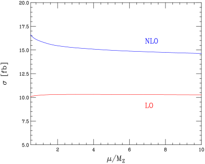
Figure 4: The scale-dependence of the leading order and next-to-leading order cross-sections $\sigma(pp\to ZZZ)$. We have set the factorization and the renormalization scales equal to a common value $\mu$.

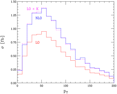
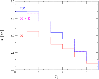
Figure 5: The transverse momentum and rapidity distributions of the $Z$ bosons at LO and NLO in $\alpha_{s}$, normalized by a factor $1/3$. The results obtained by re-scaling the LO distribution by a constant $K$-factor are also shown. The value of the factorization and the renormalization scales are set equal to $3M_{Z}$.

We now describe the results of our computation of the NLO QCD corrections to $pp\to ZZZ$. In Fig. 4 we show the dependence of the total cross-section computed through leading and next-to-leading order on the renormalization and factorization scales. We have equated these to a common scale $\mu=\mu_{R}=\mu_{F}$. There are two important features of this result to note. The first is that the corrections are large, approximately 50% over a wide range of $\mu$. This results from a large increase in the $q\bar{q}$ luminosity function when going from LO to NLO, and large virtual corrections. For example, for $\mu=3M_{Z}$, the LO cross section evaluated with LO parton distribution functions is 10.3 fb, while the LO cross section evaluated with NLO distribution functions is 11.4 fb. The full NLO result is 15.2 fb, with the additional increase coming entirely from the virtual corrections. The effect of real parton emission in the $qg$ and $\bar{q}g$ channels is 1% or less for all $\mu$ considered. We note that similarly large corrections for the process $pp\to ZZ$ at the LHC were observed in zz .

The second important feature is the tiny scale dependence of the LO result, which drastically underestimates the NLO correction. The LO result varies by only a few percent over the entire range of $\mu$ considered. While such behavior is uncommon, it is by no means unique to this process; a very similar situation occurs for $Z$ production at the Tevatron zrap .

In Fig. 5 we present the transverse momentum and rapidity distributions of the $Z$ bosons. We include all three bosons and divide by a factor of 3 to normalize the result. We compare these distributions to the approximation of reweighting the LO results by a constant $K$-factor, where $K$ is the ratio of NLO to LO inclusive cross sections. For the distributions studied, the NLO QCD corrections do not depend significantly on the kinematics of the produced particles. Rescaling the leading order kinematic distributions by a constant $K$-factor gives a description of the NLO result accurate to a few percent. We expect that this is true in all kinematic regions for which phase space is available at leading order.

V Conclusions

In this paper we present a novel numerical method for perturbative computations in QCD to next-to-leading order accuracy. We combine sector decomposition Binoth:2000ps , which allows an automatic extraction of soft and collinear singularities from virtual diagrams, with contour deformation of the Feynman parametric integrals Soper ; Soper2 , which permits numerical evaluation of loop corrections with internal thresholds. Doing so, we obtain a tool that enables an efficient and flexible numerical evaluation of Feynman diagrams with an arbitrary singularity structure. It appears to us that this combination of sector decomposition and contour deformation provides a framework in which numerical calculations of NLO virtual corrections can be fully automated.

To test this idea, we compute the next-to-leading order QCD corrections to the production of three $Z$ bosons in proton-proton collisions; this is one of the processes that appears on the so-called “NLO wishlist” NLOwish . We observe that the method possesses excellent efficiency and numerical stability; for all phase-space points considered, we were able to compute the NLO virtual corrections with sub-percent precision.

The NLO QCD corrections to $pp\to ZZZ$ are large, approximately 50% for all scale choices considered. The leading order scale dependence drastically underestimates the size of these corrections. For phase space regions accessible at leading order, the NLO corrections are independent of the kinematics of the final state particles.

Acknowledgments: K.M. is supported in part by the DOE grant DE-FG03-94ER-40833, Outstanding Junior Investigator Grant and by the Alfred P. Sloan Foundation. A.L. is supported with funds provided by the Alfred P. Sloan Foundation. F.P. is supported in part by the DOE grant DE-FG02-95ER40896, by the University of Wisconsin Research Committee with funds provided by the Wisconsin Alumni Foundation, and by the Alfred P. Sloan Foundation.

References

- (1) Talk by Bruce Knuteson at the Run2 Monte Carlo workshop, Fermilab, 2001; J. M. Campbell, J. W. Huston and W. J. Stirling, Rept. Prog. Phys. 70, 89 (2007) [arXiv:hep-ph/0611148].
- (2) G. Passarino and M. J. G. Veltman, Nucl. Phys. B 160, 151 (1979).
- (3) See, for example, V. Del Duca, W. Kilgore, C. Oleari, C. Schmidt and D. Zeppenfeld, Nucl. Phys. B 616, 367 (2001) [arXiv:hep-ph/0108030]; W. Beenakker, S. Dittmaier, M. Kramer, B. Plumper, M. Spira and P. M. Zerwas, Nucl. Phys. B 653, 151 (2003) [arXiv:hep-ph/0211352]; S. Dawson, C. Jackson, L. H. Orr, L. Reina and D. Wackeroth, Phys. Rev. D 68, 034022 (2003) [arXiv:hep-ph/0305087].
- (4) T. Binoth, J. P. Guillet, E. Pilon and M. Werlen, Eur. Phys. J. C 16, 311 (2000) [arXiv:hep-ph/9911340]; F. Cachazo, arXiv:hep-th/0410077; R. Britto, F. Cachazo and B. Feng, Phys. Lett. B 611, 167 (2005) [arXiv:hep-th/0411107]; Z. Bern, L. J. Dixon and D. A. Kosower, Phys. Rev. D 71, 105013 (2005) [arXiv:hep-th/0501240]; Z. Bern, L. J. Dixon and D. A. Kosower, Phys. Rev. D 72, 125003 (2005) [arXiv:hep-ph/0505055]; Z. Bern, L. J. Dixon and D. A. Kosower, Phys. Rev. D 73, 065013 (2006) [arXiv:hep-ph/0507005]; A. Denner and S. Dittmaier, Nucl. Phys. B 734, 62 (2006) [arXiv:hep-ph/0509141]; C. F. Berger, Z. Bern, L. J. Dixon, D. Forde and D. A. Kosower, Phys. Rev. D 75, 016006 (2007) [arXiv:hep-ph/0607014]; G. Ossola, C. G. Papadopoulos and R. Pittau, Nucl. Phys. B 763, 147 (2007) [arXiv:hep-ph/0609007].
- (5) W. T. Giele and E. W. N. Glover, JHEP 0404, 029 (2004) [arXiv:hep-ph/0402152]; F. del Aguila and R. Pittau, JHEP 0407, 017 (2004) [arXiv:hep-ph/0404120]; C. Anastasiou and A. Daleo, JHEP 0610, 031 (2006) [arXiv:hep-ph/0511176]; M. Czakon, Comput. Phys. Commun. 175, 559 (2006) [arXiv:hep-ph/0511200]; R. K. Ellis, W. T. Giele and G. Zanderighi, JHEP 0605, 027 (2006) [arXiv:hep-ph/0602185].
- (6) J. M. Campbell, R. Keith Ellis and G. Zanderighi, JHEP 0610, 028 (2006) [arXiv:hep-ph/0608194].
- (7) S. Dittmaier, P. Uwer and S. Weinzierl, arXiv:hep-ph/0703120.
- (8) Z. Bern, L. J. Dixon and D. A. Kosower, Nucl. Phys. B 513, 3 (1998) [arXiv:hep-ph/9708239]; J. Campbell, R. K. Ellis and D. L. Rainwater, Phys. Rev. D 68, 094021 (2003) [arXiv:hep-ph/0308195].
- (9) K. Hepp, Commun. Math. Phys. 2, 301 (1966).
- (10) M. Roth and A. Denner, Nucl. Phys. B 479, 495 (1996) [arXiv:hep-ph/9605420].
- (11) T. Binoth and G. Heinrich, Nucl. Phys. B 585, 741 (2000) [arXiv:hep-ph/0004013].
- (12) D. E. Soper, Phys. Rev. Lett. 81, 2638 (1998) [arXiv:hep-ph/9804454]; D. E. Soper, Phys. Rev. D 62, 014009 (2000) [arXiv:hep-ph/9910292]; D. E. Soper, Phys. Rev. D 64, 034018 (2001) [arXiv:hep-ph/0103262].
- (13) Z. Nagy and D. E. Soper, Phys. Rev. D 74, 093006 (2006) [arXiv:hep-ph/0610028].
- (14) T. Binoth, J. P. Guillet, G. Heinrich, E. Pilon and C. Schubert, JHEP 0510, 015 (2005) [arXiv:hep-ph/0504267].
- (15) P. Nogueira, J. Comput. Phys. 105, 279 (1993).
- (16) J. A. M. Vermaseren, arXiv:math-ph/0010025.
- (17) R. K. Ellis, W. J. Stirling and B. R. Webber, Camb. Monogr. Part. Phys. Nucl. Phys. Cosmol. 8, 1 (1996).
- (18) A. D. Martin, R. G. Roberts, W. J. Stirling and R. S. Thorne, Eur. Phys. J. C 23, 73 (2002) [arXiv:hep-ph/0110215]; A. D. Martin, R. G. Roberts, W. J. Stirling and R. S. Thorne, Phys. Lett. B 531, 216 (2002) [arXiv:hep-ph/0201127].
- (19) T. Hahn, Compt. Phys. Commun. 168, 78 (2005).
- (20) F. Maltoni and T. Stelzer, JHEP 0302, 027 (2003) [arXiv:hep-ph/0208156].
- (21) S. Catani, Phys. Lett. B 427, 161 (1998).
- (22) J. Ohnemus and J. F. Owens, Phys. Rev. D 43, 3626 (1991). B. Mele, P. Nason and G. Ridolfi, Nucl. Phys. B 357, 409 (1991); L. J. Dixon, Z. Kunszt and A. Signer, Phys. Rev. D 60, 114037 (1999) [arXiv:hep-ph/9907305].
- (23) C. Anastasiou, L. Dixon, K. Melnikov and F. Petriello, Phys. Rev. D69, 094008 (2004).