Abstract

We study a purely leptonic signature of the Randall–Sundrum scenario with Standard Model fields in the bulk at LHC: the contribution from the exchange of Kaluza–Klein (KK) excitations of gauge bosons to the clear Drell–Yan reaction. We show that this contribution is detectable (even with the low luminosities of the LHC initial regime) for KK masses around the TeV scale and for sufficiently large lepton couplings to KK gauge bosons. Such large couplings can be compatible with ElectroWeak precision data on the $Z\bar{f}f$ coupling in the framework of the custodial $O(3)$ symmetry recently proposed, for specific configurations of lepton localizations (along the extra dimension). These configurations can simultaneously reproduce the correct lepton masses, while generating acceptably small Flavour Changing Neutral Current (FCNC) effects. This LHC phenomenological analysis is realistic in the sense that it is based on fermion localizations which reproduce all the quark/lepton masses plus mixing angles and respect FCNC constraints in both the hadron and lepton sectors.

1 Introduction

Among the recent extra–dimensional effective scenarios, the one proposed by Randall and Sundrum (RS) [1], based on an additional warped dimension, seems quite attractive. The RS scenario provides a favorable framework for alternative models of ElectroWeak (EW) symmetry breaking, like the Higgsless [2], gauge–Higgs unification [3] or composite Higgs [4] models. From a more generic point of view, the RS scenario can address the gauge hierarchy problem without introducing any new energy scale in the fundamental theory. Moreover, the variant of the original RS model, with Standard Model (SM) fermions and bosons propagating in the bulk, allows for the unification of gauge coupling constants at a high energy Grand Unification scale [5] and provides viable candidates of Kaluza–Klein (KK) type for the dark matter of the universe [6].
In this version of the RS model with bulk matter, a purely geometrical origin arises naturally for the large mass hierarchies prevailing among SM fermions [7, 9, 8]. The principle is that if the various SM fermions are displaced along the extra dimension, their different wave function overlaps with the Higgs boson (which remains confined on the so–called TeV–brane for its mass to be protected) generate hierarchical patterns among the effective 4–dimensional Yukawa couplings. With such a geometrical approach, the quark masses and CKM mixing angles can be accommodated [9], as well as the lepton masses and MNS mixing angles in both cases where neutrinos have masses of type Majorana [10] or Dirac [11, 12] .

In the framework of the RS model with bulk fields, if the gauge hierarchy problem is to be solved, the mass of the first KK excitation of SM gauge bosons must be of order of the TeV scale. Hence, KK excitations of gauge bosons are expected to be produced significantly at the forthcoming Large Hadron Collider (LHC), which provides a center-of-mass energy of $14$ TeV, for KK gauge boson couplings to light quarks of the same order as the SM gauge couplings .

In the present work, we develop a test of KK excitation effects at LHC, in the RS scenario with bulk fields generating the SM fermion masses: we study the direct contributions of KK excitations of the photon and of the $Z$ boson to the SM Drell–Yan process, namely $pp\to\gamma^{(n)}/Z^{(n)}\to\ell^{+}\ell^{-}$, $n$ being the KK–level. The motivation for considering this process is that the neutral KK excitations can be produced as resonances, tending to increase considerably the total amplitude. Moreover, the di–lepton final state constitutes a particularly clean signature in an hadronic collider environment.
In the framework of the RS model with bulk matter, the high energy collider phenomenology and flavour physics are interestingly connected: the effective 4–dimensional couplings between KK gauge boson modes and SM fermions depend on fermion localizations along the extra–dimension which are fixed (non uniquely) by fermion masses. In the present study for the LHC, this connection between collider and flavour physics will be taken into account as we will consider some fermion location configurations which reproduce all the quark/lepton masses and mixing angles, and, satisfy Flavour Changing Neutral Current (FCNC) constraints for masses of the first KK gauge bosons around the TeV scale (see Ref. [9, 12, 16] for general discussions on these FCNC effects and Ref. [17, 18] for experimental status). This is in contrast with the preliminary study [19] on the reaction $pp\to\gamma^{(n)}/Z^{(n)}\to\ell^{+}\ell^{-}$ in the RS model, which was performed under the assumption of universal fermion locations (in order to totally avoid FCNC effects) so that SM fermion mass hierarchies were not able to be generated.

Usually, the production of heaviest SM fermions (typically localized towards the TeV–brane to have a large overlap with the Higgs boson) are considered to be favored due to their larger couplings to KK gauge bosons (also located near the TeV–brane). This has motivated recently the study, in the RS model, of the top quark pair production at LHC (through direct KK gluon production) [20, 21] and ILC (via virtual $\gamma^{(n)}/Z^{(n)}$ exchanges) [22]. Nevertheless, as will be discussed, if the left–handed charged leptons are localized closely to the TeV–brane whereas the right–handed ones are rather close to the Planck–brane, the lepton masses can still be small enough and compatible with significant couplings between left–handed charged leptons and KK gauge bosons. Such large KK couplings of leptons could be in agreement with the constraints from the EW precision data on $Z\ell\bar{\ell}$ vertex if one assumes a custodial symmetry [23, 24] and more precisely an $O(3)$ symmetry [25, 3]. This $O(3)$ symmetry will also allow to generate the heavy top mass, and simultaneously, protect the $Zb\bar{b}$ coupling as well as $\Delta\rho$ against too large corrections from KK state exchanges (the elimination of this tension was the original motivation for introducing the $O(3)$ symmetry [25]). Hence, the leptonic signature which is studied here is characteristic of the phenomenology of the RS scenario with a custodial $O(3)$ symmetry.

The paper is organized as follows. In next section, the theoretical context is described, whereas in Section 3, the relevant phenomenological constraints are discussed. The search at LHC is studied in Section 4, and conclusions are drawn in Section 5.

2 Theoretical framework

We begin by discussing the values of fundamental parameters in the RS model. While on the Planck–brane the effective gravity scale is equal to the (reduced) Planck mass: $M_{Pl}=2.44\ 10^{18}$ GeV, on the TeV–brane the gravity scale, $M_{\star}=w\ M_{Pl}$, is suppressed by the exponential ‘warp’ factor $w=e^{-\pi kR_{c}}$, where $1/k$ is the curvature radius of Anti–de–Sitter space and $R_{c}$ the compactification radius. For a small extra dimension $R_{c}\simeq 11/k$ ($k$ is taken close to $M_{Pl}$), one finds $w\sim 10^{-15}$ so that $M_{\star}={\cal O}(1)$ TeV, thus solving the gauge hierarchy problem. Solving the gauge hierarchy problem forces $M_{KK}$ (the mass of the first KK excitation of SM gauge bosons: $M_{KK}=M_{\gamma^{(1)}}\simeq M_{Z^{(1)}}$) to be of order of the TeV scale. Indeed, one has $M_{KK}=2.45kM_{\star}/M_{Pl}\lesssim M_{\star}={\cal O}(1)$ TeV since the theoretical consistency bound on the 5–dimensional curvature scalar leads to $k<0.105M_{Pl}$. More precisely, the maximal value of $M_{KK}$ is fixed by this theoretical consistency bound and the $kR_{c}$ value. One could consider a maximal value of $M_{KK}\simeq 10$ TeV which corresponds to $kR_{c}=10.11$. Since we are interested in the search for KK state effects at LHC, $M_{KK}$ will be taken instead of $k$ as the free parameter, which is equivalent.

Concerning the mass values for the SM fermions, they are dictated by their wave function location. In order to control these locations, the 5–dimensional fermion fields $\Psi_{i}$ (the generation index $i=\{1,2,3\}$) are usually coupled to distinct masses $m_{i}$ in the fundamental theory. If $m_{i}={\rm sign}(y)c_{i}k$, where $y$ parameterizes the fifth dimension and $c_{i}$ are dimensionless parameters, the fields decompose as $\Psi_{i}(x^{\mu},y)=\sum_{n=0}^{\infty}\psi_{i}^{(n)}(x^{\mu})f_{n}^{i}(y)$, where $n$ labels the tower of KK excitations and $f_{0}^{i}(y)=e^{(2-c_{i})k|y|}/N_{0}^{i}$ ($N_{0}^{i}$ being just a normalization factor). Hence, as $c_{i}$ increases, the wave function $f_{0}^{i}(y)$ tends to approach the Planck–brane at $y=0$.

We finish this section by recalling how the locations of fermions fix their effective 4–dimensional couplings to KK gauge bosons. The neutral current action of the effective 4–dimensional coupling, between SM fermions $\psi_{i}^{(0)}(x^{\mu})$ and KK excitations of any neutral gauge boson $A_{\mu}^{(n)}(x^{\mu})$, reads in the interaction basis as,

$$S_{\rm NC}=g_{L}^{SM}\int d^{4}x\sum_{n=1}^{\infty}\bar{\psi}_{Li}^{(0)}\ \gamma^{\mu}\ {\cal C}_{Lij}^{(n)}\ \psi_{Lj}^{(0)}\ A_{\mu}^{(n)}\ +\ \{L\leftrightarrow R\},$$ (1)

where $g_{L/R}^{SM}$ is the relevant SM gauge coupling constant and ${\cal C}_{Lij}^{(n)}$ the $3\times 3$ diagonal matrix $diag(C_{0}^{(n)}(c_{1}),C_{0}^{(n)}(c_{2}),C_{0}^{(n)}(c_{3}))$. These factors $C_{0}^{(n)}(c_{i})$ quantify the wave function overlap (along the extra dimension) between the localized KK excitation of gauge boson $A_{\mu}^{(n)}$ and the localized SM fermions $\psi_{i}^{(0)}$. In case of the RS model, the expression for coefficient $C_{0}^{(n)}(c_{i})$ is given e.g. by the coefficient $C_{00n}^{f_{i}\bar{f}_{i}A}$ defined in Ref. [19].
The action in Eq.(1) can be rewritten in the mass basis (indicated by the prime):

$$S_{\rm NC}=g_{L}^{SM}\int d^{4}x\sum_{n=1}^{\infty}\bar{\psi}_{L\alpha}^{(0)\ \prime}\ \gamma^{\mu}\ V_{L\alpha\beta}^{(n)}\ \psi_{L\beta}^{(0)\ \prime}\ A_{\mu}^{(n)}\ +\ \{L\leftrightarrow R\},$$ (2)

$$V_{L}^{(n)}=U_{L}^{\dagger}\ {\cal C}_{L}^{(n)}\ U_{L},$$ (3)

$U_{L}$ being the unitary matrix of basis transformation for left–handed fermions and $\alpha,\beta$ being flavour indices. One can see that the non–universality of the effective coupling constants $g_{L/R}^{SM}\times C_{0}^{(n)}(c_{i})$ between KK modes of the gauge fields and the three SM fermion families (which have different locations along $y$), in the interaction basis, induces non vanishing off–diagonal elements for matrix $V_{L/R}^{(n)}$, in the mass basis, giving rise to Flavour Changing (FC) couplings.

3 Phenomenological constraints

$\bullet$ Fermion masses: In this paper, for the purpose of illustration, three characteristic examples of complete sets for the $c_{i}$ parameter values are considered: the sets A, B and C presented in the Appendix.
The three fermion localization configurations, corresponding to sets A, B and C, have been shown in [12] to reproduce all the present data on quark/lepton masses and mixing angles (in case of Dirac neutrino masses induced by the presence of three right–handed neutrinos), through the geometrical mechanism [7] described in Section 1. The effective quark/lepton mass matrices, generated via this mechanism, depend on the $c_{i}$ and the RS parameter product $kR_{c}$, which was fixed in [12] to the same amount as here.
In particular, for these three sets, the unusually low $c_{i}^{L}$ values ($c_{i}^{L}<0.5$) for left–handed charged leptons are compensated by some large $c_{i}^{\ell}$ values for right–handed ones so that the correct electron, muon and tau masses can be generated.

$\bullet$ FCNC effects: The indirect phenomenological constraints on $M_{KK}$ holding in the RS model with bulk matter must be considered. The experimental limits on FCNC processes translate into a lower bound on $M_{KK}$. Indeed, within the context of the RS scenario creating fermion masses, FCNC processes are induced at tree level by exchanges of KK excitations of neutral gauge bosons. This is rendered possible by the fact that these KK states possess FC couplings to fermions (c.f. Eq.(2)). This is necessary as the mass hierarchies and mixings of SM fermions require flavour and nature dependent locations for quarks/leptons, or equivalently (as described in previous section), different $c_{i}$ parameter values.
The FC couplings between KK gauge bosons and SM fermions are significantly suppressed for $c_{i}$ values corresponding to certain configurations of fermion localizations [12] (see also [7, 16]). For these localization configurations, experimental limits on KK–induced FCNC effects are satisfied even for rather low KK masses. Sets A, B, C of $c_{i}$ values given in the Appendix correspond to such configurations: for these three sets of $c_{i}$ values, it was shown in [12] that FCNC reactions in both the hadron and lepton sector (like $b\to s\gamma$, $B^{0}-\bar{B}^{0}$, $\mu^{-}\to e^{-}e^{+}e^{-}$, $K\to\mu^{+}\mu^{-}$,…) respect the experimental limits if $M_{KK}\gtrsim 1$ TeV.

$\bullet$ EW measurements: Secondly, the mixing between the EW gauge bosons and their KK modes induces modifications of the boson masses/couplings, and thus deviations to EW precision observables . Hence, the fit of EW precision data imposes the typical bound $M_{KK}\stackrel{{\scriptstyle>}}{{\sim}}10$ TeV [19, 27]. Thus we first consider the scenario with the EW gauge symmetry enhanced to $SU(2)_{L}\times SU(2)_{R}\times U(1)_{X}$ [23] leading to reasonable fit of the oblique S,T parameters for $M_{KK}\stackrel{{\scriptstyle>}}{{\sim}}3$ TeV and the $c_{i}^{f_{R}}$ (for right–handed SM fermions) configurations considered in our A, B, C sets, namely $c_{i}^{d,\ell,\nu}>0.5$, $c_{1,2}^{u}>0.5$, $c_{3}^{u}<0.5$ ($i=1,\dots,3$ being the generation index). In the three sets, the low $c_{3}^{u}$ and $c_{3}^{Q}$ values (pushing typically the $t_{L/R}$,$b_{L}$ towards the TeV–brane), needed to generate the large top mass, give rise to significant $b_{L}$ couplings to KK gauge bosons. So in order to force the deviations (from both the mixing with KK gauge bosons and KK fermions) of the $Z\bar{b}_{L}b_{L}$ coupling to vanish for any $c_{3}^{Q}$ value, while still protecting the $\rho$ parameter against radiative corrections (by the already mentioned custodial $O(3)$ symmetry), the third family left–handed SM quark doublet $Q^{3}_{L}$ is embedded in a bidoublet $({\bf 2},{\bf 2})_{2/3}$ under the extended EW symmetry, as proposed in [32] and in contrast with [23]. The two other $Q^{1,2}_{L}$ light quark doublets are also embedded in bidoublets $({\bf 2},{\bf 2})_{2/3}$. Then the $u^{i}_{R}$ quarks must belong to a representation corresponding to $I_{3R}(u^{i}_{R})=I_{3L}(u^{i}_{R})=0$, which protects the $Z\bar{u}^{i}_{R}u^{i}_{R}$ vertex against any KK contribution [32]. As suggested recently in [3], the three families of left–handed SM lepton doublets $L^{i}_{L}$ are similarly embedded into bidoublets $({\bf 2},{\bf 2})_{0}$. This guarantees that there are no modifications of the $Z\bar{e}_{L}e_{L}$, $Z\bar{\mu}_{L}\mu_{L}$ and $Z\bar{\tau}_{L}\tau_{L}$ couplings, even for our chosen relatively low $c_{i}^{L}$ values that lead to a significant enhancement in the couplings between left–handed charged leptons and KK gauge bosons. If light fermions are localized far from the TeV–brane, the S parameter is positive as shown in [3] (within the gauge–Higgs unification framework). A precise analysis would be required for the case $c_{1,2}^{Q,L}<0.5$ (in the limit $c=0.5$ fermion couplings to KK gauge bosons vanish). The set A has $c^{L}$ values much smaller than $0.5$ and should be excluded by EW constraints, but we just consider it in order to illustrate a strong coupling regime.

Let us describe more precisely the lepton charges/representations under the enhanced EW gauge group $SU(2)_{L}\times SU(2)_{R}\times U(1)_{X}$ (see [32] for the quark sector). The protection of the $Z\bar{\ell}^{i}_{L}\ell^{i}_{L}$ couplings requires the equality $I_{3R}(\ell^{i}_{L})=I_{3L}(\ell^{i}_{L})$ between the $SU(2)_{R}$ and $SU(2)_{L}$ isospin quantum numbers of the charged leptons. Hence, $Q_{X}(\ell^{i}_{L})=0$ since the charge under $U(1)_{X}$ is related to the SM hypercharge $Y$ (given by $Q_{\rm em}-I_{3L}$) through: $Y=Q_{X}+I_{3R}$. Now, if the Yukawa term for charged leptons is issued from the minimal invariant operator with the form,

$$({\bf 2},{\bf 2})^{H}_{0}\overline{({\bf 2},{\bf 2})_{0}}({\bf 1},{\bf 3})_{0}$$ (4)

where $({\bf 2},{\bf 2})^{H}_{0}$ represents the Higgs boson multiplet, then $\ell^{i}_{R}\in({\bf 1},{\bf 3})_{0}\oplus({\bf 3},{\bf 1})_{0}$ with $I_{3R}(\ell^{i}_{R})=-1$. The $\ell^{i}_{R}$ representation could chosen differently at the price of generating the charged lepton masses by a non minimal operator, namely not as in Eq.(4) (an analog modification was proposed in [24, 32] for $b_{R}$ in order to solve the forward–backward anomaly of the bottom quark).
For the neutrinos, one has $I_{3R}(\nu^{i}_{L})=I_{3R}(\ell^{i}_{L})$ and, similarly, the minimal operator for the Yukawa term (neutrino masses of Dirac type are considered along this paper) has the following invariant form,

$$({\bf 2},{\bf 2})^{H}_{0}\overline{({\bf 2},{\bf 2})_{0}}({\bf 1},{\bf 1})_{0}\ \ \mbox{or}\ \ ({\bf 2},{\bf 2})^{H}_{0}\overline{({\bf 2},{\bf 2})_{0}}({\bf 1},{\bf 3})_{0}$$ (5)

where $\nu^{i}_{R}\in({\bf 1},{\bf 1})_{0}$ or $\nu^{i}_{R}\in({\bf 1},{\bf 3})_{0}\oplus({\bf 3},{\bf 1})_{0}$, respectively, with $I_{3R}(\nu^{i}_{R})=0$.

4 LHC investigation

In the following, the A, B, C sets of $c_{i}$ parameters have been considered. The important connection is that these $c_{i}$ values, determining the SM fermion wave function profiles, fix the strength of couplings between SM fermions and KK gauge bosons which dictates the amplitude of KK effects at LHC. Indeed, the dependence of this strength (Eq.(2)) on the $c_{i}$ parameters enters (Eq.(3)) via the ${\cal C}_{L/R}^{(n)}$ matrix as well as the $U_{L/R}$ matrices which diagonalize fermion mass matrices.

Only the $M_{KK}\in[3,10]$ TeV range has been considered in order to simultaneously address the gauge hierarchy problem (see Section 2) and take into account the phenomenological constraints from FCNC processes as well as EW precision data (see Section 3).

In order to compute cross sections and to generate events, the $pp\to\gamma^{(n)}/Z^{(n)}\to\ell^{+}\ell^{-}$ process has been implemented as a user defined process in the PYTHIA Monte Carlo generator version 6.205 [33]. Only the first three modes (i.e. up to the second KK excitation of the photon and of the $Z$ boson) were taken into account, as well as the interference between them. The contributions of $\gamma^{(n)}$, $Z^{(n)}$, with $n\geq 3$, to the Drell–Yan cross section are not significant because the mass (fermion couplings) of $\gamma^{(n)}$, $Z^{(n)}$ increases (decreases) as the KK–level $n$ gets higher [19]. The second KK mass is already at $M_{\gamma^{(2)}}=(5.57/2.45)M_{KK}$, and the third one is even higher.

The CTEQ5L[34] Parton Density Functions (PDF) have been used. Initial and final state radiation effects were included.

4.1 Cross sections and invariant mass distributions

The cross sections of the $pp\to\gamma^{(1,2)}/Z^{(1,2)}\to\ell^{+}\ell^{-}$ process alone (without the SM Drell–Yan contribution) computed with PYTHIA are shown as a function of $M_{KK}$ for the three parameter sets A, B and C in Fig. 1.

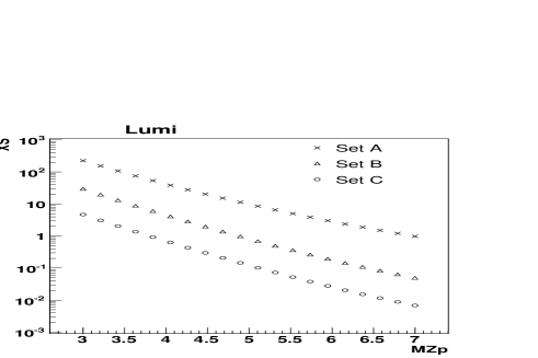
Figure 1: Cross section of the $pp\to\gamma^{(1,2)}/Z^{(1,2)}\to\ell^{+}\ell^{-}$ process ($\ell=e$ only or $\mu$ only) at LHC as a function of $M_{KK}$ for the three parameter sets A, B, C.

The $c^{L}_{i}$ parameters considered here are almost universal in the family space (namely for $i=1,2,3$) so that the wave function overlaps of left–handed leptons with KK gauge bosons, and thus the effective leptonic couplings to KK gauge bosons, are quasi identical. Furthermore, the $c^{\ell}_{i}$ are larger than $0.5$ and by consequence yield almost universal KK gauge couplings to right–handed leptons. Indeed, for $c\gg 0.5$, the ratio of KK over SM gauge coupling is fixed at $\sim-0.2$ since the KK gauge boson wave functions are quasi constant near the Planck-brane. Therefore, the cross sections for the different lepton generations are practically equal, after having also taken into account the dependence of effective KK gauge couplings on lepton mixing angles (parameterizing the $U$ matrices of Eq.(2)-(3)).
On the other hand, one can see that the cross section gets higher when moving from set C to set B, and then to set A. The reason is that, the $c^{Q,L}_{i}$ values of set C are larger (this is not the case for the right–handed top quark, or more precisely $c_{3}^{u}$, but the top is not involved in the studied reaction) than in set B and in turn larger than in set A, so that for this latter set the left–handed light fermions are localized closer to the TeV–brane, where are also located KK gauge bosons, leading to larger KK gauge couplings. Concerning the other $c$ parameters, those are larger than $0.5$ leading to almost universal KK gauge couplings, as already discussed.

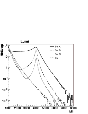
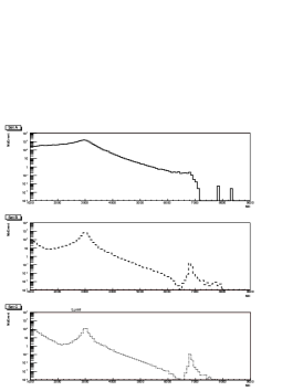
Figure 2: Left: distribution of the generated invariant mass $M_{\ell\ell}$ ($\ell=e$ only or $\mu$ only) for the $pp\to\gamma^{(0,1,2)}/Z^{(0,1,2)}\to\ell^{+}\ell^{-}$ process at LHC, with $M_{KK}=4$ TeV and parameter sets A (plain line), B (dashed line) or C (dotted line). The absolute number of events corresponds to an integrated luminosity of ${\cal L}=100$ fb^-1. The same invariant mass distribution for the pure SM process $pp\to\gamma^{(0)}/Z^{(0)}\to\ell^{+}\ell^{-}$ (dot–dashed line) is also shown. Right: same distribution with $M_{KK}=3$ TeV.

Figure 2 (left) shows the generated distribution of the final state di–lepton invariant mass $M_{\ell\ell}=\sqrt{(p_{\ell^{+}}+p_{\ell^{-}})^{2}}$ obtained for sets A, B, C with $M_{KK}=4$ TeV. The resonance peak around $M_{\ell\ell}=M_{KK}$ is clearly visible above a relatively small physical background, the SM Drell–Yan process. Moreover, the $pp\to\gamma^{(0,1,2)}/Z^{(0,1,2)}\to\ell^{+}\ell^{-}$ process yields a large number of events for an integrated luminosity ${\cal L}=100$ fb^-1, which corresponds to one year of LHC running at high luminosity. Even lower integrated luminosities would lead to a significant number of events. The difference of KK gauge boson widths between the three parameter sets originates from the difference in KK gauge couplings. It must be noticed also that there is a destructive interference between the SM and RS contributions which reduces the number of events, with respect to the pure Drell–Yan process, at invariant masses lower than the resonance level.

Figure 2 (right) shows the generated distribution of the final state di–lepton invariant mass for $M_{KK}=3$ TeV for the three parameter sets separately. The second resonance peak, due to the exchange of $\gamma^{(2)}$ and $Z^{(2)}$ excitations, appears around $M_{\ell\ell}=(5.57/2.45)M_{KK}$. Its experimental detection would be characteristic of a tower of massive KK states, and would thus represent a strong indication for the existence of extra dimensions. Together with a measurement of the $\gamma^{(2)}/Z^{(2)}$ mass, it would constitute a clear signature of the specific RS model with bulk matter. However, the amplitude for $\gamma^{(2)}/Z^{(2)}$ production is highly suppressed by the decrease of PDFs at large parton energies.

4.2 Detectability

In order to study the detectability of such events at LHC, the expected performance of the ATLAS detector [35] has been used. This performance has been computed using a full simulation of the detector response [36]. The response to the particles out of the tracking acceptance (i.e. with a pseudo-rapidity $|\eta|>2.5$) was not simulated. The events were then reconstructed in the official ATLAS reconstruction framework [36].

We concentrate here on the electron final state, which we have already studied in detail in the framework of other models [37]. The muon and tau lepton cases will be commented at the end of this section. A $\gamma^{(n)}/Z^{(n)}\to e^{+}e^{-}$ event selection and reconstruction is designed and the efficiency of such a selection is evaluated as explained in the next subsection. Finally, the ATLAS discovery reach is computed, as shown in the last subsection.

Event selection and selection efficiency

The same selection as in [37] is used. First the electron (positron) candidates are reconstructed using the standard ATLAS electron identification: additionally to criteria on shower shape and energy leakage, one requires to have a good track quality. The absence of any additional track in a broad cone around the matched track is also required in order to reduce the QCD and tau backgrounds.

Only events with at least two electron candidates are selected. These two candidates are also required to be isolated in the calorimeter, which means that no more than 40 GeV have been deposited in the calorimeter in a cone of radius $\sqrt{(\Delta\eta)^{2}+(\Delta\phi)^{2}}=0.5$ around the electron direction. Finally, the two electrons are required to be of opposite charge and back to back in the plane transverse to the beam, the absolute difference of azimuthal angles having to be greater than 2.9 radians.

These criteria are aimed at selecting di–electron events and rejecting possible background events. After this selection, Drell–Yan events, indistinguishable from $\gamma^{(n)}/Z^{(n)}$ events are expected to be the only physical background. Some non–physical, reducible background could come from processes such as $\gamma W$ events in which the photon is misidentified as an electron and the $W$ decays into an electron. Given their cross section and the rejecting power of the electron identification, they are assumed to be negligible.

The final efficiency of the selection on signal events is shown as a function of the di–electron invariant mass on Fig. 3. Two curves are shown separately for $u\bar{u}$ and $d\bar{d}$ events because the events arising from $u\bar{u}$ fusion are slightly more boosted than those arising from $d\bar{d}$ fusion (because of their PDFs). Provided that one separates these two contributions, it has been shown that the selection efficiencies are model independent [37]. In both cases, the efficiency is relatively flat as a function of the di–electron invariant mass. No electron was simulated above 4.5 TeV but the performance is expected to remain about the same for higher energies, even if this implies some initial adjustments.

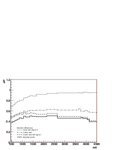
Figure 3: Selection efficiency as a function of $M_{ee}$; left: $u\bar{u}$ events, right: $d\bar{d}$ events.

ATLAS discovery reach

As seen on the invariant mass distribution, the resonance shows a large bump which can be detected by searching for an excess of events above the expected spectrum from the SM process. One could also exploit the fact that there is a strong destructive interference at di–lepton invariant masses lower than the resonance by looking for a deficit of events. For simplicity sake, we restrict here to the search for an excess, but we note that the sensitivity could possibly be improved by designing a search for a deficit.

The expected number of signal events ($S$) and of background events ($B$) is evaluated in the following invariant mass interval: [$M_{thr},\infty$[, where $M_{thr}=0.6M_{KK}$ has been optimized in order to integrate the full signal in the case of set A, which has the largest natural width.

In order to compute $S$ and $B$, events have been generated by PYTHIA and efficiency weighted according to $M_{\ell\ell}$ and to the incoming quark flavour in order to derive an effective production cross section. This procedure was also applied to the irreducible background. A significance estimator, called $S_{12}$, was finally used in order to extract the discovery reach. This estimator is defined by $2S_{12}=2(\sqrt{S+B}-\sqrt{B})$; this definition has been shown [38] to be less optimistic than the usual $S/\sqrt{B}$. The discovery is claimed if the two following conditions are met: $2S_{12}>5$ and $S>10$.

In order to make a full computation of the discovery reach, it would be necessary to consider possible systematic effects. These are of various kinds, either experimental such as the uncertainty on the integrated luminosity, the electron energy scale, etc, or theoretical, such as higher order corrections to the cross section computation. This is beyond the scope of this paper, and will be treated elsewhere [39]. The results obtained here are thus dominated by the cross section.

The value of the $M_{KK}$ reach is shown as a function of the integrated luminosity on Fig. 4. One can see that the ATLAS discovery potential for the exchange of KK neutral gauge bosons is sizable, even for low integrated luminosities. For instance, the medium coupled B set is detectable up to about 4 TeV with only 10 fb^-1 of integrated luminosity, which could be reached after a couple of years of running. The reach extends up to about 5.8 TeV for the same model with 300 fb^-1.

From the theoretical point of view, the cross sections for electron and muon productions are almost the same, as explained in Section 4.1. Experimentally, a study of the muon detection efficiency based on a fast simulation has showed that this efficiency should be comparable to the electron one. Hence, one can estimate that including the statistics of the muon final state would be roughly equivalent to multiplying the integrated luminosity by a factor of 2, so that the above reaches would be obtained with twice as less luminosity.
The rates for electron and tau leptons are also similar. However, the detection of the tau lepton, which is unstable, is experimentally more difficult than the detection of the light stable leptons and would require a specific analysis. Even if no such specific selection is performed, the leptonic decays of the di–tau final state would contribute to the high mass di–lepton spectrum. However, given the branching ratios, the final significance, and in turn the sensitivity on $M_{KK}$, is not expected to vary significantly.

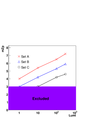
Figure 4: ATLAS discovery reach in the electron final state in terms of $M_{KK}$ as a function of the integrated luminosity for parameter sets A, B, C.

5 Conclusion

We have considered several configurations of SM fermion localizations, in the RS model, which generate a realistic structure in flavour space (reproducing quark/lepton masses and satisfying FCNC bounds for low $M_{KK}$). We have noticed that these configurations also possess the particularity of producing lepton couplings to KK gauge bosons which are larger than in the SM and can remain in agreement with the EW precision data if one assumes a custodial $O(3)$ symmetry. Then, based on these different fermion configurations, we have shown that the experimental search at LHC for new effects in the SM Drell–Yan process coming from exchanges of KK gauge bosons would lead to a high sensitivity on $M_{KK}$ up to $\sim 6$ TeV (depending on the scenario and considered luminosity) due to the clean leptonic signature. Such effects would constitute an indication for the existence of the O(3) symmetry.

Appendix

We denote set A the following set of $c_{i}$ values for each SM fermion,

$$\begin{array}[]{cccccc}c_{1}^{Q}=0.2\ ;&c_{2}^{Q}=0.2\ ;&c_{3}^{Q}=0.2&c_{1}^{L}=-1.5\ ;&c_{2}^{L}=-1.5\ ;&c_{3}^{L}=-1.5\\ c_{1}^{d}=0.728\ ;&c_{2}^{d}=0.740\ ;&c_{3}^{d}=0.628&c_{1}^{\ell}=0.760\ ;&c_{2}^{\ell}=0.833\ ;&c_{3}^{\ell}=0.667\\ c_{1}^{u}=0.62\ ;&c_{2}^{u}=0.62\ ;&c_{3}^{u}=0.35&c_{1}^{\nu}=1.512\ ;&c_{2}^{\nu}=1.513\ ;&c_{3}^{\nu}=1.468\end{array}$$

whereas set B is defined by,

$$\begin{array}[]{cccccc}c_{1}^{Q}=0.37\ ;&c_{2}^{Q}=0.37\ ;&c_{3}^{Q}=0.37&c_{1}^{L}=0.200\ ;&c_{2}^{L}=0.200\ ;&c_{3}^{L}=0.261\\ c_{1}^{d}=0.716\ ;&c_{2}^{d}=0.728\ ;&c_{3}^{d}=0.615&c_{1}^{\ell}=0.737\ ;&c_{2}^{\ell}=0.696\ ;&c_{3}^{\ell}=0.647\\ c_{1}^{u}=0.607\ ;&c_{2}^{u}=0.607\ ;&c_{3}^{u}=0.050&c_{1}^{\nu}=1.496\ ;&c_{2}^{\nu}=1.503\ ;&c_{3}^{\nu}=1.463\end{array}$$

and set C is given by,

$$\begin{array}[]{cccccc}c_{1}^{Q}=0.413\ ;&c_{2}^{Q}=0.413\ ;&c_{3}^{Q}=0.413&c_{1}^{L}=0.35\ ;&c_{2}^{L}=0.35\ ;&c_{3}^{L}=0.39\\ c_{1}^{d}=0.703\ ;&c_{2}^{d}=0.721\ ;&c_{3}^{d}=0.608&c_{1}^{\ell}=0.728\ ;&c_{2}^{\ell}=0.694\ ;&c_{3}^{\ell}=0.636\\ c_{1}^{u}=0.60\ ;&c_{2}^{u}=0.60\ ;&c_{3}^{u}=-0.08&c_{1}^{\nu}=1.49\ ;&c_{2}^{\nu}=1.49\ ;&c_{3}^{\nu}=1.45\end{array}$$

References

- [1] L. Randall and R. Sundrum, Phys. Rev. Lett. 83 (1999) 3370; M. Gogberashvili, Int. J. Mod. Phys. D11 (2002) 1635.
- [2] C. Csaki et al., Phys. Rev. Lett. 92 (2004) 101802; R. Barbieri et al., Phys. Lett. B591 (2004) 141; G. Cacciapaglia et al., Phys.Rev. D75 (2007) 015003 .
- [3] M. Carena, E. Pontón, J. Santiago and C. E. M. Wagner, Nucl. Phys. B759 (2006) 202; arXiv: hep-ph/0701055.
- [4] R. Contino et al., Nucl. Phys. B671 (2003) 148; arXiv: hep-ph/0612048; K. Agashe et al., Nucl. Phys. B719 (2005) 165.
- [5] A. Pomarol, Phys. Rev. Lett. 85 (2000) 4004; L. Randall and M. D. Schwartz, JHEP 0111 (2001) 003; Phys. Rev. Lett. 88 (2002) 081801; W. D. Goldberger and I. Z. Rothstein, Phys. Rev. D68 (2003) 125011; K. Choi and I.-W. Kim, Phys. Rev. D67 (2003) 045005; K. Agashe, A. Delgado and R. Sundrum, Annals Phys. 304 (2003) 145.
- [6] K. Agashe and G. Servant, Phys. Rev. Lett. 93 (2004) 231805; JCAP 0502 (2005) 002.
- [7] T. Gherghetta and A. Pomarol, Nucl. Phys. B586 (2000) 141.
- [8] Y. Grossman and M. Neubert, Phys. Lett. B474 (2000) 361; G. Moreau, Eur. Phys. J. C40 (2005) 539; T. Appelquist et al., Phys. Rev. D65 (2002) 105019; T. Gherghetta, Phys. Rev. Lett. 92 (2004) 161601.
- [9] S. J. Huber and Q. Shafi, Phys. Lett. B498 (2001) 256; S. J. Huber, Nucl. Phys. B666 (2003) 269; S. Chang, C. S. Kim and M. Yamaguchi, Phys. Rev. D73 (2006) 033002, arXiv: hep-ph/0511099.
- [10] S. J. Huber and Q. Shafi, Phys. Lett. B544 (2002) 295; Phys. Lett. B583 (2004) 293.
- [11] S. J. Huber and Q. Shafi, Phys. Lett. B512 (2001) 365; G. Moreau and J. I. Silva-Marcos, JHEP 0601 (2006) 048;
- [12] G. Moreau and J. I. Silva-Marcos, JHEP 0603 (2006) 090.
- [13] C. Dennis et al., arXiv: hep-ph/0701158.
- [14] A. L. Fitzpatrick et al., arXiv: hep-ph/0701150.
- [15] K. Agashe et al., arXiv: hep-ph/0701186.
- [16] K. Agashe et al., Phys. Rev. Lett. 93 (2004) 201804; Phys. Rev. D71 (2005) 016002.
- [17] Z. Ligeti, M. Papucci and G. Perez, Phys. Rev. Lett. 97 (2006) 101801; K. Agashe et al., arXiv: hep-ph/0509117; K. Agashe et al., Phys. Rev. D74 (2006) 053011; arXiv: hep-ph/0606293.
- [18] P. M. Aquino et al., arXiv: hep-ph/0612055.
- [19] H. Davoudiasl, J. L. Hewett and T. G. Rizzo, Phys. Rev. D63 (2001) 075004.
- [20] K. Agashe, A. Belyaev, T. Krupovnickas, G. Perez and J. Virzi, arXiv: hep-ph/0612015.
- [21] B. Lillie, L. Randall and L.-T. Wang, arXiv: hep-ph/0701166.
- [22] E. De Pree and M. Sher, Phys. Rev. D73 (2006) 095006.
- [23] K. Agashe, A. Delgado, M. J. May and R. Sundrum, JHEP 0308 (2003) 050.
- [24] A. Djouadi, G. Moreau and F. Richard, to appear in Nucl. Phys. B (2007), arXiv: hep-ph/0610173.
- [25] K. Agashe, R. Contino, L. Da Rold and A. Pomarol, Phys. Lett. B641 (2006) 62.
- [26] A. Delgado and A. Falkowski, arXiv: hep-ph/0702234.
- [27] G. Burdman, Phys. Rev. D66 (2002) 076003.
- [28] F. del Aguila, M. Perez-Victoria and J. Santiago, JHEP 0302 (2003) 051.
- [29] M. Carena, T. M. P. Tait and C. E. M. Wagner, Acta Phys. Polon. B33 (2002) 2355.
- [30] M. Carena, E. Ponton, T. M. P. Tait and C. E. M. Wagner, Phys. Rev. D67 (2003) 096006; M. Carena et al., Phys. Rev. D68 (2003) 035010.
- [31] M. Carena et al., Phys. Rev. D71 (2005) 015010.
- [32] K. Agashe, R. Contino, L. Da Rold and A. Pomarol, Phys. Lett. B641 (2006) 62.
- [33] T. Sjostrand, S. Mrenna and P. Skands, JHEP 0605 (2006) 026. arXiv: hep-ph/0603175.
- [34] H.L. Lai et al., Phys. Rev. D51 (1995) 4763.
- [35] ATLAS Collaboration, ATLAS detector and physics performance Technical Design Report, CERN/LHCC 99-15, 1999.
-
[36]
ATLAS Computing Group, ATLAS Computing Technical Design Report,
CERN-LHCC-2005-022, 2005.
The version used here corresponds to the Data Challenge 1 (DC1). - [37] F. Ledroit, J. Morel and B. Trocmé, ATL-PHYS-PUB-2006-024, also in V. Buescher et al., Tevatron-for-LHC Report: Preparations for Discoveries, arXiv: hep-ph/0608322.
- [38] S. I. Bityukov and N. V. Krasnikov, Nucl. Instrum. Meth. A452 518 (2000) 518.
- [39] K. Black et al, ATLAS CSC note, in preparation.