Abstract

We study the LHC discovery potential for heavy Majorana neutrino singlets in the process $pp\to W^{+}\to\ell^{+}N\to\ell^{+}\ell^{+}jj$ ($\ell=e,\mu$) plus its charge conjugate. With a fast detector simulation we show that backgrounds involving two like-sign charged leptons are not negligible and, moreover, they cannot be eliminated with simple sequential kinematical cuts. Using a likelihood analysis it is shown that, for heavy neutrinos coupling only to the muon, LHC has $5\sigma$ sensitivity for masses up to 200 GeV in the final state $\mu^{\pm}\mu^{\pm}jj$. This reduction in sensitivity, compared to previous parton-level estimates, is driven by the $\sim 10^{2}-10^{3}$ times larger background. Limits are also provided for $e^{\pm}e^{\pm}jj$ and $e^{\pm}\mu^{\pm}jj$ final states, as well as for Tevatron. For heavy Dirac neutrinos the prospects are worse because backgrounds involving two opposite charge leptons are much larger. For this case, we study the observability of the lepton flavour violating signal $e^{\pm}\mu^{\mp}jj$. As a by-product of our analysis, heavy neutrino production has been implemented within the ALPGEN framework.

1 Introduction

Large hadron colliders involve strong interacting particles as initial states, giving rise to huge hadronic cross sections. The large luminosities expected will also provide quite large electroweak signals, with for instance $1.6\times 10^{10}$ ($4\times 10^{7}$) $W$ bosons at LHC (Tevatron) for a luminosity of 100 (2) fb^-1. Therefore, these colliders can be used for precise studies of the leptonic sector as well, and in particular they can produce new heavy neutrinos at an observable level, or improve present limits on their masses and mixings [1, 2, 3, 4] (see Ref. [5] for a review). These new fermions transform trivially under the gauge symmetry group of the Standard Model (SM), and in the absence of other interactions they are produced and decay only through their mixing with the SM leptons. With new interactions, like for instance in left-right models [6], heavy neutrinos can be produced by gauge couplings unsuppressed by small mixing angles, yielding larger cross sections and implying a much higher collider discovery reach [7, 8, 9, 10]. Heavy neutrinos could also be copiously produced in pairs through the exchange of a relatively light $Z^{\prime}$ boson [11]. In these scenarios, however, the observation of the new interactions could be more interesting than the existence of new heavy neutrinos.

We will concentrate on the first possibility and neglect other new production mechanims, taking a conservative approach. In this case, for example, it has been claimed by looking at the lepton number violating (LNV) $\Delta L=2$ process $pp^{\!\!\!\!\!\textsuperscript{\tiny{(--)}}}\!\!\rightarrow\mu^{\pm}\mu^{\pm}jj$ that LHC will be sensitive to heavy Majorana neutrinos with masses $m_{N}$ up to 400 GeV, whereas Tevatron is sensitive to masses up to 150 GeV [2, 4]. However, as we will show, taking into account the actual backgrounds these limits are far from being realistic. In particular, backgrounds involving $b$ quarks, including for instance $t\bar{t}nj$ (with $nj$ standing for $n=0,1,2,\dots$ additional jets), are two orders of magnitude larger than previously estimated. Moreover, in the region $m_{N}<M_{W}$ the largest and irreducible background is $b\bar{b}nj$, by far dominant but overlooked in previous parton-level analyses [4]. In this work we make a detailed study, at the level of fast simulation, of the LHC sensitivity to Majorana neutrinos in the process $pp\rightarrow\mu^{\pm}\mu^{\pm}jj$, which is the cleanest final state, for both $m_{N}>M_{W}$ and $m_{N}<M_{W}$. We also study the processes $pp\to e^{\pm}e^{\pm}jj$ and $pp\to e^{\pm}\mu^{\pm}jj$ for which the sensitivity is slightly worse. Heavy Dirac neutrinos do not produce LNV signals and then their observation is much more difficult. As an example, we examine the lepton flavour violating (LFV) signal $e^{\pm}\mu^{\mp}jj$, produced by a heavy Dirac neutrino coupling to the electron and muon.

The generation of heavy neutrino signals has been implemented in the ALPGEN [12] framework, including the process studied here as well as other final states. In the following, after making precise our assumptions and notation in section 2, we describe the implementation of heavy neutrino production in ALPGEN in section 3. We present our detailed results in section 4, where we will eventually find that heavy neutrinos can be discovered up to masses of the order of 200 GeV, and that for $N$ lighter than the $W$ boson its mixing can be probed at the $10^{-2}$ level (for a “reference” mass $m_{N}=60$ GeV). These figures are much less optimistic than in previous literature. Estimates for Tevatron are given in section 5, and our conclusions are drawn in section 6. In two appendices we detail the evaluation of the $b\bar{b}nj$ background and the heavy neutrino mass reconstruction, respectively.

2 Heavy neutrino interactions

Our assumptions and notation are reviewed in more detail in Ref. [5] (see also Refs. [13, 14]). The SM is only extended with heavy neutrino singlets $N_{j}$, which are assumed to have masses of the order of the electroweak scale, up to few hundreds of GeV. We concentrate on the lightest one, assuming for simplicity that the other extra neutrinos are heavy enough to neglect possible interference effects. The new heavy neutrino $N$ (where we suppress the unnecessary subindex) can have Dirac character, what requires the addition of at least two singlets, or Majorana, in which case $(N_{L})^{c}\equiv CN_{L}^{T}=N_{R}$ and lepton number is violated. In either case it is produced and decays through its mixing with the light leptons, which is described by the interaction Lagrangian (in standard notation)

$$\mathcal{L}_{W} = -\frac{g}{\sqrt{2}}\left(\bar{\ell}\gamma^{\mu}V_{\ell N}P_{L}N\;W_{\mu}+\bar{N}\gamma^{\mu}V_{\ell N}^{*}P_{L}\ell\;W_{\mu}^{\dagger}\right)\,,$$

$$\mathcal{L}_{Z} = -\frac{g}{2c_{W}}\left(\bar{\nu}_{\ell}\gamma^{\mu}V_{\ell N}P_{L}N+\bar{N}\gamma^{\mu}V_{\ell N}^{*}P_{L}\nu_{\ell}\right)Z_{\mu}\,,$$

$$\mathcal{L}_{H} = -\frac{g\,m_{N}}{2M_{W}}\,\left(\bar{\nu}_{\ell}\,V_{\ell N}P_{R}N+\bar{N}\,V_{\ell N}^{*}P_{L}\nu_{\ell}\right)H\,.$$ (1)

The SM Lagrangian remains unchanged in the limit of small mixing angles $V_{\ell N}$, $\ell=e,\mu,\tau$ (which is the actual case), up to very small corrections $O(V^{2})$. Neutral couplings involving two heavy neutrinos are also of order $V^{2}$. The heavy neutrino mass $m_{N}$ joins two different bispinors in the Dirac case and the same one in the Majorana case. Heavy neutrino decays are given by their interactions in Eqs. (1): $N\to W^{+}\ell^{-}$, $N\to Z\nu$, $N\to H\nu$, plus $N\to W^{-}\ell^{+}$ for a heavy Majorana neutrino. For $m_{N}<M_{W}$ all these decays produce three body final states, mediated by off-shell $W$, $Z$ or $H$ bosons. The total width for a Majorana neutrino is twice larger than for a Dirac one with the same couplings [15, 16, 17, 5].

As it is apparent from Eqs. (1), heavy neutrino signals are proportional to the neutrino mixing with the SM leptons $V_{\ell N}$. Limits on these matrix elements have been extensively discussed in previous literature, and we quote here only the main results. Low-energy data constrain the quantities

$$\Omega_{\ell\ell^{\prime}}\equiv\delta_{\ell\ell^{\prime}}-\sum_{i=1}^{3}V_{\ell\nu_{i}}V_{\ell^{\prime}\nu_{i}}^{*}=\sum_{j=1}^{n}V_{\ell N_{j}}V_{\ell^{\prime}N_{j}}^{*}\,.$$ (2)

A global fit to tree level processes involving light neutrinos as external states gives [18, 19],

$$\Omega_{ee}\leq 0.0054\,,\quad\Omega_{\mu\mu}\leq 0.0096\,,\quad\Omega_{\tau\tau}\leq 0.016$$ (3)

at 90% confidence level (CL). Note that a global fit without the unitarity bounds implies $\Omega_{ee}\leq 0.012$ [18]. Additionally, for Majorana neutrinos coupling to the electron the experimental bound on neutrinoless double beta decay requires [20]

$$\left|\,\sum_{j=1}^{n}\,V_{eN_{j}}^{2}\,\frac{1}{m_{N_{j}}}\,\right|\,<5\times 10^{-8}\;{\rm GeV}^{-1}\,.$$ (4)

If $V_{eN_{j}}$ saturate $\Omega_{ee}$ in Eq. (3), this limit can be satisfied either demanding that $m_{N_{j}}$ are large enough, beyond the TeV scale [21] and then beyond LHC reach, or that there is a cancellation among the different terms in Eq. (4), as may happen in definite models [22], in particular for (quasi)Dirac neutrinos.

Flavour changing neutral processes further restrict $\Omega_{\ell\ell^{\prime}}$. The new contributions, and then the bounds, depend on the heavy neutrino masses. In the limit $m_{N_{j}}^{2}\gg M_{W}^{2}\gg|V_{\ell N_{j}}|^{2}m_{N_{j}}^{2}$ they imply [24]

$$|\Omega_{e\mu}|\leq 0.0001\,,\quad|\Omega_{e\tau}|\leq 0.01\,,\quad|\Omega_{\mu\tau}|\leq 0.01\,.$$ (5)

Except in the case of $\Omega_{e\mu}$, for which experimental constraints on lepton flavour violation are rather stringent, these limits are similar to the limits on the diagonal elements. An important difference, however, is that (partial) cancellations among loop contributions of different heavy neutrinos may be at work [25]. Cancellations with other new physics contributions are also possible. Since we are interested in determining the heavy neutrino discovery potential and the direct limits on neutrino masses and mixings which can be eventually established, we must consider the largest possible neutrino mixings, although they may require model dependent cancellations or fine-tuning.

3 Heavy neutrino production with ALPGEN

For the signal event generation we have extended ALPGEN [12] with heavy neutrino production. This Monte Carlo generator evaluates tree level SM processes and provides unweighted events suitable for simulation. A simple way of including new processes taking advantage of the ALPGEN framework is to provide the corresponding squared amplitudes decomposed as a sum over the different colour structures. In the case of heavy neutrinos this is trivial because there is only one term. This method requires to evaluate from the beginning the squared amplitudes for the processes one is interested in, what is done using HELAS [26]. An alternative possibility which gives more flexibility for future applications is to implement the new vertices at the same level as the SM ones, what is quite more involved.

We have restricted ourselves to single heavy neutrino production. Pair production is suppressed by an extra $V^{2}$ mixing factor and by the larger center of mass energy required, what implies smaller PDFs and more suppressed $s$-channel propagators. Single heavy neutrino production can proceed through $s$-channel $W,Z$ or $H$ exchange. The first two production mechanisms have been implemented in ALPGEN for the various possible final states given by the heavy neutrino decays $N\to W^{\pm}\ell^{\mp}$, $N\to Z\nu_{\ell}$, $N\to H\nu_{\ell}$ with $\ell=e,\mu,\tau$, and for both Dirac or Majorana $N$. In the case $m_{N}<M_{W}$ all decays are three-body, and mediated by off-shell $W$, $Z$ or $H$. The transition from two-body to three-body decays on the $M_{W}$, $M_{Z}$ and $M_{H}$ thresholds is smooth, since the calculation of matrix elements and the $N$ width are done for off-shell intermediate bosons. Two approximations are made, however. The small mixing of heavy neutrinos with charged leptons implies that their production is dominated by diagrams with $N$ on-shell, like those shown in Fig. 1, with a pole enhancement factor, and that non-resonant diagrams are negligible. (Additionally, to isolate heavy neutrino signals from the background one expects that the heavy neutrino mass will have to be reconstructed to some extent.) Then, the only diagrams included are the resonant ones. In the calculation we also neglect light fermion masses except for the bottom quark.

(a)		(b)

Figure 1: Feynman diagrams for the process $q\bar{q}^{\prime}\to\ell^{+}N$, followed by LNV decay $N\to\ell^{(^{\prime})+}W^{-}$ (a) and lepton number conserving (LNC) decay $N\to\ell^{(^{\prime})-}W^{+}$ (b). The diagrams for the charge conjugate processes are similar.

Generator-level results are presented in Fig. 2 for LHC and Tevatron in the relevant mass ranges. Solid lines correspond to the total $\mu N$ cross sections for $|V_{\mu N}|=0.098$, $V_{eN}=V_{\tau N}=0$. The dashed lines are the cross sections for the final state $\mu^{\pm}\mu^{\pm}jj$, which is the cleanest one. The dotted lines are the same but with kinematical cuts

$$\mathrm{LHC}:\begin{array}[]{ccc}p_{T}^{\mu}\geq 10~{}\mathrm{GeV}\,,&|\eta^{\mu}|\leq 2.5\,,&\Delta R_{\mu j}\geq 0.4\,,\\ p_{T}^{j}\geq 10~{}\mathrm{GeV}\,,&|\eta^{j}|\leq 2.5\,,\end{array}$$ (8)

$$\mathrm{Tevatron}:\begin{array}[]{ccc}p_{T}^{\mu}\geq 10~{}\mathrm{GeV}\,,&|\eta^{\mu}|\leq 2\,,&\Delta R_{\mu j}\geq 0.4\,,\\ p_{T}^{j}\geq 10~{}\mathrm{GeV}\,,&|\eta^{j}|\leq 2.5\,,\end{array}$$ (11)

included to reproduce roughly the acceptance of the detector and give approximately the “effective” size of the observable signal. Of course, the correct procedure is to perform a simulation, as we do in next section, but for illustrative purposes we include the cross-sections after cuts. In particular, they clearly show that although for $m_{N}<M_{W}$ the total cross sections grow several orders of magnitude, both at LHC and Tevatron, partons tend to be produced with low transverse momenta (the two muons and two quarks result from the decay of an on-shell $W$), making the observable signal much smaller. These results are in agreement with those previously obtained in Ref. [4].

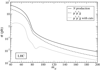
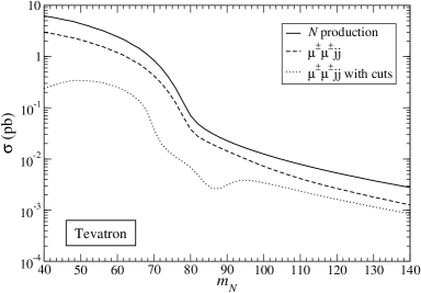
Figure 2: Cross sections for heavy neutrino production at LHC (left) and Tevatron (right), as a function of the heavy neutrino mass, for $|V_{\mu N}|=0.098$. The solid lines correspond to total $\mu N$ cross section, the dashed lines include the decay to like-sign muons and the dotted lines are the same but including the kinematical cuts in Eq. (11).

4 Di-lepton signals at LHC

The most interesting scenario for LHC is when the heavy neutrino has Majorana nature and couples only to the muon, so that it produces a final state $\mu^{\pm}\mu^{\pm}jj$ with two same sign muons and at least two jets. Since this LNV signal has sometimes been considered [2, 4] to be almost background free (more realistic background estimates are given in Ref. [27]), a detailed discussion of the actual backgrounds is worthwhile. A first group of processes involves the production of additional leptons, either neutrinos or charged leptons (which may be missed in the detector). The main ones are $W^{\pm}W^{\pm}nj$ and $W^{\pm}Znj$. We point out that not only the processes with $n=2$ contribute: processes with $n<2$ are backgrounds due to the appearance of extra jets from pile-up, and processes with $n>2$ cannot be cleanly removed because of pile-up on the signal. A second group includes final states with $b$ and/or $\bar{b}$ quarks, like $t\bar{t}nj$, with semileptonic decay of the $t\bar{t}$ pair, and $Wb\bar{b}nj$, with $W$ decaying leptonically. In these cases the additional like-sign muon results from the decay of a $b$ or $\bar{b}$ quark. Only a tiny fraction of such decays produce isolated muons with sufficiently high transverse momentum. But, since the $t\bar{t}nj$ and $Wb\bar{b}nj$ cross sections are so large, these backgrounds are also much larger than backgrounds with two weak gauge bosons. Finally, $b\bar{b}nj$ production is several orders of magnitude larger than all processes mentioned above, but the produced muons have small $p_{T}$ and invariant mass in this case. Then, in general it might be eliminated with suitable high-$p_{T}$ cuts on charged leptons [28] (see section 4.1), but for $m_{N}<M_{W}$ the heavy neutrino signal is also characterised by very small transverse momenta (see section 4.2), and this background turns out to be the dominant one. The same applies for $c\bar{c}nj$, but with the difference that $c$ quark decays produce isolated charged leptons much less often than $b$ decays.

Other LNV signals produced by heavy neutrinos are $e^{\pm}e^{\pm}jj$ and $e^{\pm}\mu^{\pm}jj$. They have the same SM backgrounds but with one important difference: $b$ decays produce “apparently isolated” electrons more often than muons, because electrons are detected in the calorimeter while muons travel to the muon chamber. Hence, the corresponding backgrounds $t\bar{t}nj,b\bar{b}nj\to e^{\pm}e^{\pm}X/e^{\pm}\mu^{\pm}X$ are larger than the ones involving only muons. A precise evaluation of these backgrounds, optimising the criteria for electron isolation, seems to require a full simulation of the detector. The limits provided in these cases must be regarded with some caution in this respect, and should be confirmed with a full detector simulation.

We have generated the signal and backgrounds using ALPGEN and passing them through PYTHIA 6.4 [29] with the MLM prescription [30] to avoid double counting of jet radiation. A fast simulation of the ATLAS detector [31] has been performed. For the signal and all backgrounds except $b\bar{b}nj$ and $c\bar{c}nj$ the number of simulated events corresponds to at least 10 times the luminosity considered (which is 30 fb^-1), so as to reduce statistical fluctuations, and the number of events is scaled accordingly. For $b\bar{b}nj$ and $c\bar{c}nj$ the luminosity simulated is 0.075 fb^-1. Their evaluation is further discussed in appendix A. It must also be noted that in the signal simulation all $W$ decays in $pp\to\ell N\to\ell\ell^{\prime}W$ are included. Leptonic $W$ decays give an extra $\sim 20\%$ contribution to di-lepton final states when the charged lepton from the $W$ decay is missed, or when $W$ decays to $\tau\nu$ and the tau lepton decays hadronically.

4.1 $\ell^{\pm}\ell^{\pm}jj$ production for $m_{N}>M_{W}$

In this mass region we take the reference values $m_{N}=150$ GeV and (a) $V_{\mu N}=0.098$, $V_{eN}=V_{\tau N}=0$; (b) $V_{eN}=0.073$, $V_{\mu N}=V_{\tau N}=0$; (c) $V_{eN}=0.073$, $V_{\mu N}=0.098$, $V_{\tau N}=0$. The pre-selection criteria used for our analysis are:

• two like-sign isolated charged leptons with pseudorapidity $|\eta^{\ell}|\leq 2.5$ and transverse momentum $p_{T}^{\ell}$ larger than 10 GeV (muons) or 15 GeV (electrons), and no additional isolated charged leptons;

• no additional non-isolated muons;

• two jets with $|\eta^{j}|\leq 2.5$ and $p_{T}^{j}\geq 20$ GeV.

We point out that for $\mu^{\pm}\mu^{\pm}jj$ final states the requirement (ii) reduces the backgrounds involving $Z$ bosons by almost a factor of two, and thus proves to be quite useful. The number of events at LHC for 30 fb^-1 after pre-selection cuts is given in Table 1. Additional backgrounds such as $t\bar{b}$, $t\bar{t}t\bar{t}$, $t\bar{t}b\bar{b}$, $Zt\bar{t}nj$, $WWZnj$, $WZZnj$ and $ZZZnj$ are smaller and we do not show them, but they are included in the estimation of the signal significance below. The number of like-sign dimuon events from $c\bar{c}nj$ displayed between parentheses corresponds to an estimation, because no $\mu^{\pm}\mu^{\pm}X$ events are found in the sample simulated (more details can be found in appendix A). We also note that the higher $p_{T}$ threshold for electrons contributes to the difference between the numbers of $e^{\pm}e^{\pm}jj$ and $\mu^{\pm}e^{\pm}jj$ events, which are expected to be similar in some cases, for example for $t\bar{t}nj$.

	Pre-selection				Selection
	$\mu^{\pm}\mu^{\pm}$	$e^{\pm}e^{\pm}$	$\mu^{\pm}e^{\pm}$		$\mu^{\pm}\mu^{\pm}$	$e^{\pm}e^{\pm}$	$\mu^{\pm}e^{\pm}$
$N~{}(\mathrm{a})$	113.6	0	0		59.1	0	0
$N~{}(\mathrm{b})$	0	72.0	0		0	17.6	0
$N~{}(\mathrm{c})$	78.4	25.5	82.6		41.6	4.7	22.4
$b\bar{b}nj$	14800	52000	82000		0	0	0
$c\bar{c}nj$	(11)	300	200		(0)	0	0
$t\bar{t}nj$	1162.1	8133.0	15625.3		2.4	8.3	7.7
$tj$	60.8	176.5	461.5		0.0	0.0	0.1
$Wb\bar{b}nj$	124.9	346.7	927.3		0.4	0.6	0.3
$Wt\bar{t}nj$	75.7	87.2	166.9		0.3	0.0	0.0
$Zb\bar{b}nj$	12.2	68.9	117.0		0.0	0.2	0.0
$WWnj$	82.8	89.0	174.8		0.5	0.1	0.7
$WZnj$	162.4	252.0	409.2		4.8	1.8	2.3
$ZZnj$	3.8	13.3	12.9		0.0	0.6	0.1
$WWWnj$	31.9	30.1	64.8		0.9	0.1	0.0

Table 1: Number of $\ell^{\pm}\ell^{\pm}jj$ events at LHC for 30 fb^-1, at the pre-selection and selection levels. The heavy neutrino signal is evaluated assuming $m_{N}=150$ GeV and coupling (a) to the muon, $V_{\mu N}=0.098$; (b) to the electron, $V_{eN}=0.073$; (c) to both, $V_{eN}=0.073$ and $V_{\mu N}=0.098$.

Let us concentrate on $\mu^{\pm}\mu^{\pm}jj$ final states. The fast simulation shows that SM backgrounds are about two orders of magnitude larger than previously estimated (three orders if we include $b\bar{b}nj$). Moreover, they cannot be sufficiently suppressed with respect to the heavy neutrino signal using simple cuts. Some obvious discriminating variables are:

• The missing momentum ${p\!\!\!\!\!\not\,\,\,\,}_{T}$. It is smaller for the signal because it does not have neutrinos in the final state, but nonzero due to energy mismeasurement in the detector.

• The separation between the muon with smallest $p_{T}$ (we label the two muons as $\mu_{1}$, $\mu_{2}$, by decreasing transverse momentum) and the closest jet, $\Delta R_{\mu_{2}j}$. For backgrounds involving high-$p_{T}$ $b$ quarks this separation tends to be rather small.

• The transverse momentum of the two muons, $p_{T}^{\mu_{1}}$ and $p_{T}^{\mu_{2}}$, respectively. In particular $p_{T}^{\mu_{2}}$ is a good discriminant against backgrounds from $b$ quarks, because these typically have one muon with small $p_{T}$.

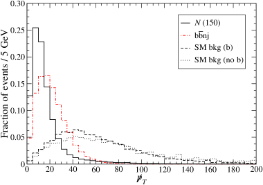
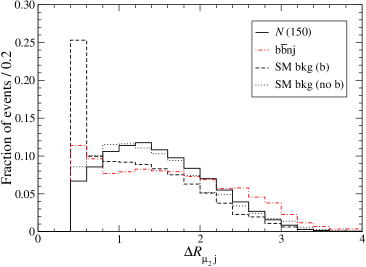
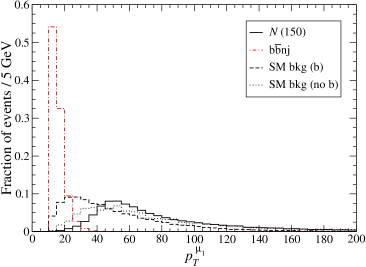
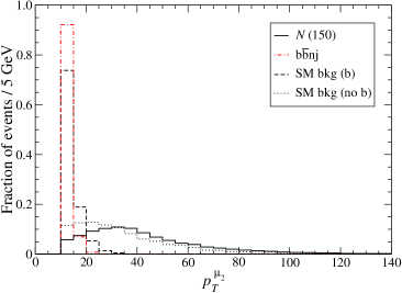
Figure 3: Normalised distributions of several discriminating variables for the $\mu^{\pm}\mu^{\pm}jj$ signal with $m_{N}=150$ GeV and its backgrounds (see the text).

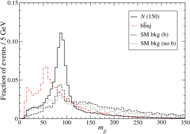
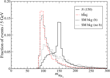
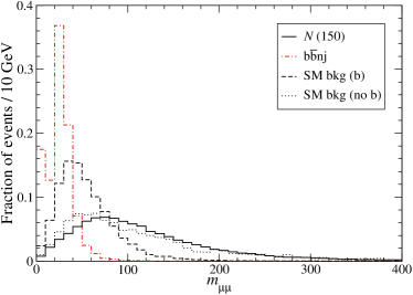
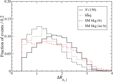
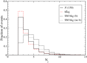
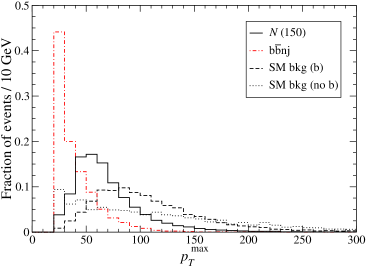
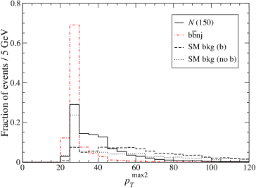
Figure 4: Normalised distributions of several discriminating variables for the $\mu^{\pm}\mu^{\pm}jj$ signal with $m_{N}=150$ GeV and its backgrounds (see the text).

These variables are plotted in Fig. 3 for the $\mu^{\pm}\mu^{\pm}jj$ signal and the backgrounds grouped in three classes with common features: (a) $b\bar{b}nj$, where both muons come from $b$ quark decays (the contribution of $c\bar{c}nj$ is negligible); (b) $t\bar{t}nj$, $tj$ and $W/Zb\bar{b}nj$, where one muon comes from a $b$ quark; (c) backgrounds where both muons come from $W/Z$ decays (mainly di-boson and tri-boson production). Kinematical cuts on the variables listed above do not render the $\mu^{\pm}\mu^{\pm}jj$ final state “background free”, as it is apparent from the plots (and we have explicitly checked). Indeed, for the large background cross sections in Table 1 the overlapping regions contain a large number of background events, and they can be eliminated only by severely reducing the signal. However, a likelihood analysis using these and further variables can efficiently reduce the background. The additional variables are shown in Fig. 4:

• The invariant mass $m_{jj}$ of the two jets with largest transverse momentum, which for the signal are assumed to originate from the $W$ hadronic decay, and the invariant mass of $\mu_{2}$ (the muon with lowest $p_{T}$) and these two jets, $m_{W\mu_{2}}$. (Further details about the $W$ and $N$ mass reconstruction can be found in appendix B.) An important observation in this case is that in backgrounds involving $b$ quarks this muon typically has a small $p_{T}$, displacing the background peaks to lower invariant masses.

• The invariant mass of the two muons.

• The separation between the muon with largest $p_{T}$ and the closest jet, $\Delta R_{\mu_{1}j}$.

• The number of $b$-tagged jets $N_{b}$ and jet multiplicities $N_{j}$. Especially the former helps to separate the backgrounds involving $b$ quarks because they often have $b$-tagged jets. In this fast simulation analysis we have fixed the $b$-tagging efficiency to 60%, but in a full simulation the $b$ tag probability can be included in the likelihood function, improving the discriminating power of this variable.

• The transverse momenta of the two jets with largest $p_{T}$, $p_{T}^{\mathrm{max}}$ and $p_{T}^{\mathrm{max2}}$ respectively.

These variables are not suited for performing kinematical cuts but greatly improve the discriminating power of a likelihood function. The resulting log-likelihood function is also shown in Fig. 5, where we distinguish four likelihood classes as in the previous figures: the signal, $b\bar{b}nj$, backgrounds with one muon from $b$ decays, and backgrounds with both muons from $W/Z$ decays.

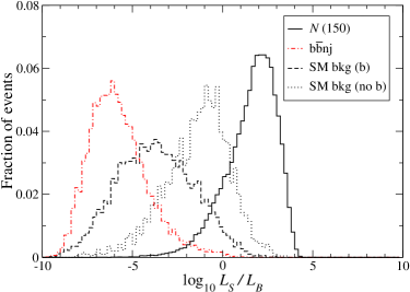
Figure 5: Log-likelihood function for the $\mu^{\pm}\mu^{\pm}jj$ signal with $m_{N}=150$ GeV and its backgrounds.

The probability distributions built for $\mu^{\pm}\mu^{\pm}jj$ final states are used for $e^{\pm}e^{\pm}jj$ and $\mu^{\pm}e^{\pm}jj$ as well. As selection criteria we require $\log_{10}L_{S}/L_{B}\geq 1.4$ for $\mu^{\pm}\mu^{\pm}jj$ and $\log_{10}L_{S}/L_{B}\geq 2.5$ for $e^{\pm}e^{\pm}jj$ and $\mu^{\pm}e^{\pm}jj$ final states, respectively, and that at least one of the two heavy neutrino mass assignments $m_{W\mu_{1}}$, $m_{W\mu_{2}}$ is between 130 and 170 GeV. The number of events surviving these cuts can be read on the right part of Table 1. As it is apparent, the likelihood analysis is quite effective in suppressing backgrounds, especially $b\bar{b}nj$, $t\bar{t}nj$ and $W/Zb\bar{b}nj$. The resulting statistical significance for the heavy neutrino signals are collected in Table 2, assuming a “reference” 20% systematic uncertainty in the backgrounds (which still has to be precisely evaluated in a dedicated study).

	$\mu^{\pm}\mu^{\pm}$	$e^{\pm}e^{\pm}$	$\mu^{\pm}e^{\pm}$
$N~{}(\mathrm{a})$	$16.2\sigma$	$-$	$-$
$N~{}(\mathrm{b})$	$-$	$4.2\sigma$	$-$
$N~{}(\mathrm{c})$	$11.4\sigma$	$1.1\sigma$	$5.5\sigma$

Table 2: Statistical significance of the heavy neutrino signals in the different channels, for a mass $m_{N}=150$ GeV and coupling (a) to the muon, $V_{\mu N}=0.098$; (b) to the electron, $V_{eN}=0.073$; (c) to both, $V_{eN}=0.073$ and $V_{\mu N}=0.098$.

The limits on heavy neutrino masses and couplings depend on the light lepton they are coupled to. We can consider two extreme cases:

• A 150 GeV heavy neutrino coupling only to the muon can be discovered for mixings $|V_{\mu N}|\geq 0.054$, and if no background excess is found the limits $|V_{\mu N}|^{2}\leq 0.97\;(1.2)\times 10^{-3}$ can be set at 90% (95%) CL, improving the ones from low energy processes (see section 2) by a factor of 10. Heavy neutrino masses up to 200 GeV can be observed with $5\sigma$ at the LHC for $V_{\mu N}=0.098$.

• A 150 GeV heavy neutrino coupling only to the electron can be discovered for mixings $|V_{eN}|\geq 0.080$ (excluded by the limits in section 2), but if no background excess is found the limits $|V_{eN}|^{2}\leq 2.1\;(2.5)\times 10^{-3}$, which are slightly better than the one derived from Eq. (3), can be set at 90% (95%) CL. Heavy neutrino masses up to 145 GeV can be observed with $5\sigma$ at the LHC for $V_{eN}=0.073$.

For a heavy neutrino coupling to the electron and muon the limits depend on both couplings as well as on its mass. The combined limits for $m_{N}=150$ GeV are displayed in Fig. 6. Except in the regions with $V_{eN}\sim 0$ or $V_{\mu N}\sim 0$, the indirect limit from $\mu-e$ LFV processes, also shown in this plot, is much more restrictive.

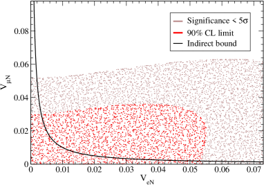
Figure 6: Combined limits on $V_{eN}$ and $V_{\mu N}$, for $V_{\tau N}=0$ and $m_{N}=150$ GeV. The red areas represent the 90% CL limits if no signal is observed. The white areas correspond to the region where a combined statistical significance of $5\sigma$ or larger is achieved. The indirect limit from $\mu-e$ LFV processes is also shown.

These limits can be considered conservative in the sense that only the lowest-order signal contribution (without hard extra jets at the partonic level) has been included, and further signal contributions $\ell Nnj$ should improve the heavy neutrino observability. If the Higgs is heavier than 120 GeV the branching ratios $\mathrm{Br}(N\to W\ell)$ will increase as well. We also stress again that in the $e^{\pm}e^{\pm}jj$ and $\mu^{\pm}e^{\pm}jj$ channels the evaluation of $t\bar{t}nj$ and other backgrounds with isolated electrons from $b$ quarks must be confirmed with a full simulation, with an eventual optimisation of the isolation criteria. This is beyond the scope of the present work.

It is worth explaining here in more detail why our results are much more pessimistic than previous ones. With this purpose, we apply to signal and backgrounds the sequential kinematical cuts in Ref. [4]:

• Missing energy ${p\!\!\!\!\!\not\,\,\,\,}_{T}<25$ GeV.

• Lego-plot separation $\Delta R_{\mu j}>0.5$.

• Dijet invariant mass $60~{}\text{GeV}<m_{jj}<100~{}\text{GeV}$, where the two jets are expected to come from the $W$ boson in the case of the signal.

The number of events for the signal and main backgrounds after these cuts are gathered in the left column of Table 3 (we do not show smaller backgrounds for brevity). For $m_{N}=150$ GeV and $V_{\mu N}=0.098$ the signal cross section is reduced to 1.7 fb, to be compared to $\sim 2.2$ fb in Ref. [4]. But our total background cross section after cuts amounts to 44 fb, while their estimate is of 0.04 fb. This difference by a factor of $1000$ arises mainly from the $b\bar{b}nj$ background, overlooked before, which is by far the largest one. But even if $b\bar{b}nj$ is not taken into account, the background cross section $\sim 0.88$ fb is 20 times larger, due to: (i) $t\bar{t}nj$, which was assumed negligible after cuts, and $W/Zb\bar{b}nj$, also overlooked; (ii) the $WZnj$ background, because parton-level analyses underestimate the probability of missing a lepton and thus its contribution; (iii) pile-up, which makes lower order processes ($n<2$) contribute. All these backgrounds, collected in Table 3, can be compared to $WWW$, which was found to be the main background before. The resulting statistical significance of the signal, ignoring systematic errors, is $S/\sqrt{B}=1.41\sigma$ for 30 fb^-1, far from the $\sim 30\sigma$ previously estimated. (If one makes the more realistic assumption that systematic errors are of order 20%, as we do in this work, then the statistical significance is further reduced to $0.19\sigma$.) It could be argued that the cuts in the previous list might be strengthened in order to further reduce the backgrounds. But this would be at the cost of reducing the signal as well. On the other hand, additional cuts on lepton transverse momenta can be introduced to reduce $b\bar{b}nj$ and $t\bar{t}nj$. Requiring that one charged lepton has $p_{T}\geq 30$ GeV and the other one $p_{T}\geq 20$ GeV, the signal is hardly affected while $b\bar{b}nj$ is essentially eliminated, as it is shown in the second column of Table 3. The statistical significance in this case is $S/\sqrt{B}=14.1\sigma$ (ignoring systematic errors) or $12.1\sigma$ (with 20% systematics). We emphasise that, as it can be observed by comparing Tables 1 and 3, a probabilistic analysis is much more powerful in this case than a standard one based on cuts. But at any rate recovering parton-level estimates for the signal significance seems hardly possible.

	Sequential cuts I	Sequential cuts II
$N~{}(\mu)$	51.3	44.0
$b\bar{b}nj$	1293	2.7
$t\bar{t}nj$	15.3	1.4
$Wb\bar{b}nj$	3.6	0.2
$Wt\bar{t}nj$	0.7	0.7
$Zb\bar{b}nj$	0.9	0.0
$WWnj$	0.5	0.5
$WZnj$	4.1	2.9
$WWWnj$	1.1	0.9

Table 3: Number of $\mu^{\pm}\mu^{\pm}jj$ events at LHC for 30 fb^-1, after the kinematical cuts in Ref. [4] (first column) and with additional requirements (second column, see the text). The heavy neutrino signal is evaluated assuming $m_{N}=150$ GeV and $V_{\mu N}=0.098$.

Finally, we would like to note that we have not addressed the observability of heavy neutrino signals in $\tau$ lepton decay channels because they are expected to have much worse sensitivity. For hadronic $\tau$ decays the charge of the decaying lepton seems rather difficult to determine, hence backgrounds from top pair and $Z$ production will be huge (see also section 4.3 below). For leptonic decays $\tau\to\ell\nu_{\tau}\bar{\nu}_{\ell}$, $\ell=e,\mu$, not only the branching ratios are smaller, but also the signal has final state neutrinos and thus the discriminating power of ${p\!\!\!\!\!\not\,\,\,\,}_{T}$ against di-boson and tri-boson backgrounds is much worse.

4.2 $\ell^{\pm}\ell^{\pm}jj$ production for $m_{N}<M_{W}$

In this mass region we take the reference values $m_{N}=60$ GeV and (a) $V_{\mu N}=0.01$, $V_{eN}=V_{\tau N}=0$; (b) $V_{eN}=0.01$, $V_{\mu N}=V_{\tau N}=0$; (c) $V_{eN}=0.01$, $V_{\mu N}=0.01$, $V_{\tau N}=0$. The pre-selection criteria are the same as before. The likelihood analysis is performed distinguishing four classes: the signal, $b\bar{b}nj$, backgrounds with one muon from $b$ decays, and backgrounds with both muons from $W/Z$ decays. The relevant variables are depicted in Figs. 7 and 8:

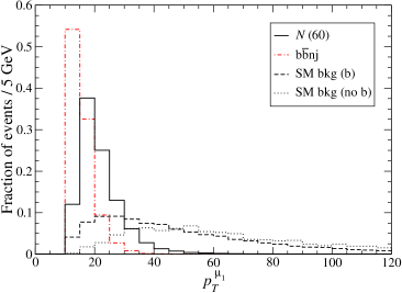
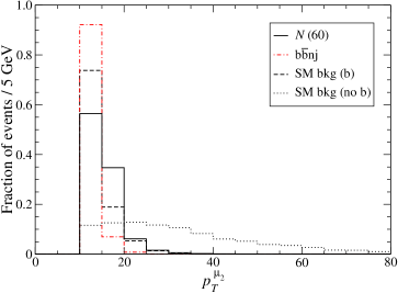
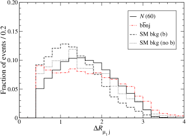
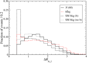
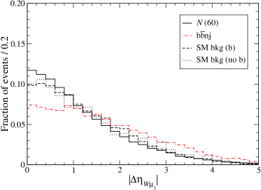
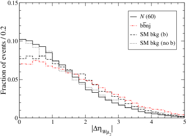
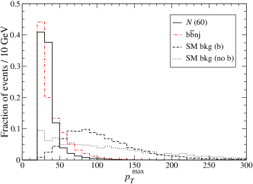
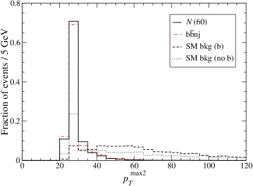
Figure 7: Normalised distributions of several discriminating variables for the $m_{N}=60$ GeV signal and the three background classes (see the text).

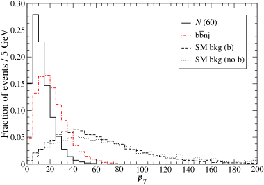
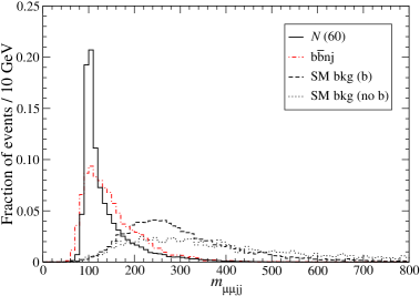
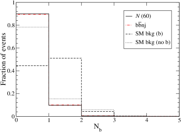
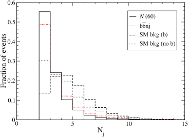
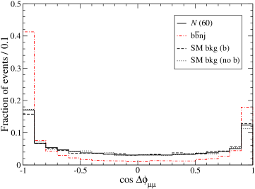
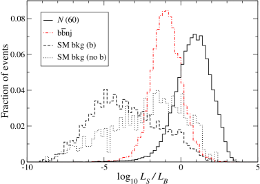
Figure 8: Normalised distributions of several discriminating variables for the $m_{N}=60$ GeV signal and the three background classes (see the text). The last plot corresponds to the log-likelihood function.

• The transverse momenta of the two muons (slightly smaller for $b\bar{b}nj$ than for the signal, and much larger for the other backgrounds).

• The distance between them and the closest jet, which is a good discriminator against $t\bar{t}nj$ but not against $b\bar{b}nj$.

• The rapidity difference between the muons and the $W^{*}$ from $N$ decay, which is reconstructed from the two jets with highest $p_{T}$.

• The transverse momenta of the two jets with largest $p_{T}$. Again, these two variables are excellent discriminators against high-$p_{T}$ backgrounds like $t\bar{t}nj$ and di-boson production, but not very useful for $b\bar{b}nj$.

• The missing transverse momentum.

• The invariant mass of the two muons and two jets with highest $p_{T}$, $m_{\mu\mu jj}$. For the signal, these four particles result from the decay of an on-shell $W$ boson, so the distribution is very peaked around 100 GeV (the position of the peak is displaced as a consequence of pile-up, which generates jets with larger $p_{T}$ than the ones from the signal itself). Unfortunately, for $b\bar{b}nj$ the distribution is quite similar.

• The number of $b$ tags and the jet multiplicity.

• The azimuthal angle (in transverse plane) between the two muons, $\phi_{\mu\mu}$. For $b\bar{b}$ without additional jets this angle is often close to $180^{\circ}$, but for $b\bar{b}j$ and higher order processes (which are also huge) this no longer holds.

The resulting log-likelihood function is presented in Fig. 8. As it can be easily noticed with a quick look at the variables presented, the kinematics of $b\bar{b}nj$ is very similar to the signal and so this background is very difficult to eliminate. In particular, for larger $m_{N}$ requiring large transverse momentum for the leptons drastically reduces $b\bar{b}nj$ (as seen in the previous subsection), but for $m_{N}<M_{W}$ it reduces significantly the signal as well. As selection cut we require $\log_{10}L_{S}/L_{B}\geq 2.2$ for the three final states, which practically eliminates all backgrounds except $b\bar{b}nj$. The number of remaining background events is given in the right part of Table 4 (numbers of background events at pre-selection equal those in Table 1, and are quoted on the left for better comparison).

	Pre-selection				Selection
	$\mu^{\pm}\mu^{\pm}$	$e^{\pm}e^{\pm}$	$\mu^{\pm}e^{\pm}$		$\mu^{\pm}\mu^{\pm}$	$e^{\pm}e^{\pm}$	$\mu^{\pm}e^{\pm}$
$N~{}(\mathrm{a})$	427.3	0	0		42.1	0	0
$N~{}(\mathrm{b})$	0	174.7	0		0	33.9	0
$N~{}(\mathrm{c})$	214.0	88.5	290.9		20.4	17.1	39.3
$b\bar{b}nj$	14800	52000	82000		10.7	291	96
$c\bar{c}nj$	(11)	300	200		(0)	0	0
$t\bar{t}nj$	1162.1	8133.0	15625.3		0.3	1.3	1.3
$tj$	60.8	176.5	461.5		0.0	0.0	0.1
$Wb\bar{b}nj$	124.9	346.7	927.3		0.2	2.4	1.3
$Wt\bar{t}nj$	75.7	87.2	166.9		0.0	0.0	0.0
$Zb\bar{b}nj$	12.2	68.9	117.0		0.0	1.4	0.2
$WWnj$	82.8	89.0	174.8		0.0	0.0	0.0
$WZnj$	162.4	252.0	409.2		0.6	0.4	0.5
$ZZnj$	3.8	13.3	12.9		0.0	0.5	0.1
$WWWnj$	31.9	30.1	64.8		0.9	0.0	0.0

Table 4: Number of $\ell^{\pm}\ell^{\pm}jj$ events at LHC for 30 fb^-1, at the pre-selection and selection levels. The heavy neutrino signal is evaluated assuming $m_{N}=60$ GeV and coupling (a) to the muon, $V_{\mu N}=0.01$; (b) to the electron, $V_{eN}=0.01$; (c) to both, $V_{eN}=0.01$ and $V_{\mu N}=0.01$.

Requiring larger $L_{S}/L_{B}$ for the $e^{\pm}e^{\pm}jj$ and $\mu^{\pm}e^{\pm}jj$ channels does not improve the results, because it decreases the signals too much. The resulting statistical significance for the heavy neutrino signals are collected in Table 5, assuming a 20% systematic uncertainty in the backgrounds.

	$\mu^{\pm}\mu^{\pm}$	$e^{\pm}e^{\pm}$	$\mu^{\pm}e^{\pm}$
$N~{}(\mathrm{a})$	$10.0\sigma$	$-$	$-$
$N~{}(\mathrm{b})$	$-$	$0.54\sigma$	$-$
$N~{}(\mathrm{c})$	$4.9\sigma$	$0.28\sigma$	$1.75\sigma$

Table 5: Statistical significance of the heavy neutrino signals in the different channels, for a mass $m_{N}=60$ GeV and coupling (a) to the muon, $V_{\mu N}=0.01$; (b) to the electron, $V_{eN}=0.01$; (c) to both, $V_{eN}=0.01$ and $V_{\mu N}=0.01$.

From these significances, the following limits can be extracted:

• A 60 GeV neutrino coupling only to the muon can be discovered for mixings $|V_{\mu N}|\geq 0.0070$, and bounds $|V_{\mu N}|^{2}\leq 1.65(1.95)\times 10^{-5}$ can be set at 90% (95%) CL if a background excess is not observed. These figures are $\sim 35$ times worse than in previous parton-level estimates which overlooked the main background $b\bar{b}nj$, but would still improve the direct limit from L3 [32, 33] by an order of magnitude.

• A 60 GeV neutrino coupling only to the electron can be discovered for mixings $|V_{eN}|\geq 0.030$, and bounds $|V_{eN}|^{2}\leq 3.1(3.6)\times 10^{-4}$ can be set at 90% (95%) CL if a background excess is not observed.

The general limits for a heavy neutrino coupling to the electron and muon are displayed in Fig. 9. It is interesting to observe that the direct limit from non-observation of like-sign dileptons at LHC will be more restrictive than indirect ones from $\mu-e$ LFV processes at low energies.

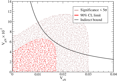
Figure 9: Combined limits on $V_{eN}$ and $V_{\mu N}$, for $V_{\tau N}=0$ and $m_{N}=60$ GeV. The red areas represent the 90% CL limits if no signal is observed. The white areas correspond to the region where a combined statistical significance of $5\sigma$ or larger is achieved. The indirect limit from $\mu-e$ LFV processes is also shown.

4.3 Opposite-sign dilepton signals

In final states $e^{\pm}\mu^{\mp}jj$ the analysis is similar but the backgrounds are much larger. In particular, opposite-sign lepton pairs from $b\bar{b}nj$ production are much more abundant than like-sign pairs. Opposite-sign dileptons are produced from $t\bar{t}nj$ dileptonic decays and $W^{+}W^{-}nj$ production (which is larger than $W^{\pm}W^{\pm}nj$). We assume a heavy Dirac neutrino with a mass of 60 GeV and $V_{eN}=0.01$, $V_{\mu N}=0.01$. A Majorana neutrino gives this signal too, but with half the cross section for the same couplings. We use the same pre-selection cuts as in the like-sign dilepton analysis but requiring instead opposite charge for the leptons. The number of signal and background events at pre-selection is collected in the left column of Table 6. At pre-selection the $b\bar{b}nj$, $t\bar{t}nj$ and $WWnj$ backgrounds are 7, 15 and 70 times larger, respectively, than the corresponding ones for $\mu^{\pm}e^{\mp}$ in Table 4.

	Pre-selection		Selection
$N~{}(e,\mu)$	593.5		14.7
$b\bar{b}nj$	602000		73
$c\bar{c}nj$	5750		0
$t\bar{t}nj$	233135.1		0.3
$tj$	1003.8		0.0
$Wb\bar{b}nj$	927.6		0.0
$Wt\bar{t}nj$	197.0		0.0
$Zb\bar{b}nj$	180.8		0.0
$WWnj$	12016.5		0.7
$WZnj$	412.1		0.0
$ZZnj$	14.2		0.0
$WWWnj$	131.4		0.0

Table 6: Number of $\mu^{\pm}e^{\mp}jj$ events at LHC for 30 fb^-1, at the pre-selection and selection levels. The heavy neutrino signal is evaluated assuming $m_{N}=60$ GeV and coupling to electron and muon $V_{eN}=0.01$, $V_{\mu N}=0.01$.

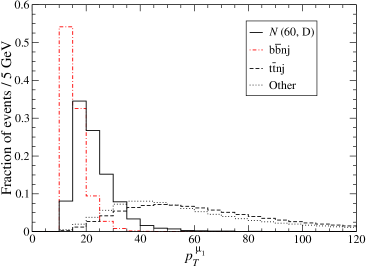
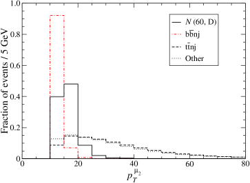
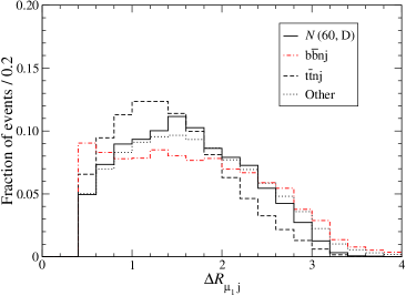
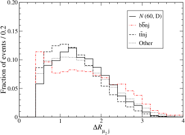
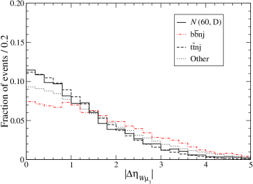
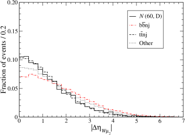
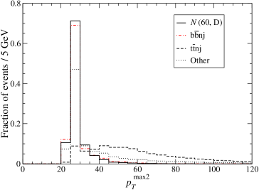
Figure 10: Normalised distributions of several discriminating variables for a 60 GeV Dirac neutrino and the three background classes (see the text).

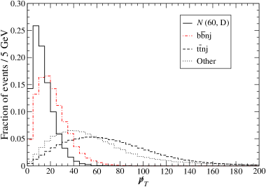
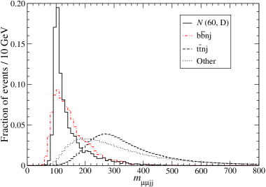
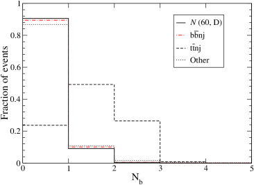
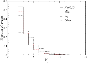
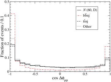
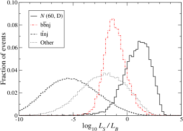
Figure 11: Normalised distributions of several discriminating variables for a 60 GeV Dirac neutrino and the three background classes (see the text). The last plot corresponds to the log-likelihood function.

The kinematical variables useful for discriminating the signal against the backgrounds are the same as for a 60 GeV heavy Majorana neutrino in the like-sign dilepton channels. However, in this case the distributions for some backgrounds, namely $t\bar{t}nj$ and $WWnj$, are different. We have grouped backgrounds in three classes: $b\bar{b}nj$, $t\bar{t}nj$, and the other backgrounds (dominated by $WWnj$). The distributions for the relevant kinematical variables and the log-likelihood function are collected in Figs. 10 and 11. For event selection we require $\log_{10}L_{S}/L_{B}\geq 2.9$, yielding the number of events in the right columns of Table 6. The significance of the heavy Dirac neutrino signal is only $0.86\sigma$. The combined limits on $V_{eN}$ and $V_{\mu N}$ are presented in Fig. 12. The shape of the regions is drastically different from Figs. 6 and 9 because the sensitivity in the $e^{+}e^{-}jj$ and $\mu^{+}\mu^{-}jj$ channels is negligible, and only when $N$ couples sizeably to both electron and muon the heavy neutrino signal is statistically significant in the $\mu^{\pm}e^{\mp}jj$ channel. The direct limit from non-observation of a $\mu^{\pm}e^{\mp}jj$ excess has a similar shape as the indirect limit but it is less restrictive in all cases.

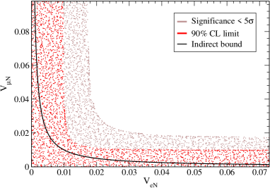
Figure 12: Combined limits on $V_{eN}$ and $V_{\mu N}$ for a 60 GeV Dirac neutrino. The red areas represent the 90% CL limits if no signal is observed. The white areas correspond to the region where a combined statistical significance of $5\sigma$ or larger is achieved. The indirect limit from $\mu-e$ LFV processes is also shown.

5 Estimates for Tevatron

The observability of heavy neutrino signals in like-sign dilepton channels at Tevatron seems to be dominated by the size of the signal itself. In contrast with LHC, backgrounds are much smaller. For example, the $WZjj$ and $WWjj$ backgrounds have cross sections of 0.1 and 0.09 fb, respectively, with the cuts in Eq. (11). Then, it seems reasonable to estimate the total background for 1 fb^-1 (including $b\bar{b}$) as one event. This rough estimation is in agreement with the detailed calculation in Ref. [34], in which $b\bar{b}$ is estimated from real data. Therefore, if signal events have not been observed with the already collected luminosity, upper limits of 3.36 and 4.14 events [35] can be set on the signal, at 90% and 95% CL, respectively. From Fig. 2, and for a fixed mass $m_{N}=60$ GeV, this implies upper bounds $|V_{\mu N}|^{2}\leq 1.3\times 10^{-4}$ (90% CL) $|V_{\mu N}|^{2}\leq 1.6\times 10^{-4}$ (95% CL). This would slightly improve the limits from L3 [32, 33]. Of course, a detailed simulation with the already collected data is necessary to make any claim, and the limits eventually obtained will depend on the actual number of observed like-sign dilepton events.

Note also that, given the cross sections in Fig. 2, for a luminosity of 1 fb^-1 and $V_{\mu N}=0.098$ the heavy neutrino signals only exceed a handful of events for heavy neutrino masses $m_{N}<M_{W}$, and thus the Tevatron sensitivity (when acceptance and efficiency are taken into account) is limited to this mass range. This also holds for a heavy neutrino mixing with the tau lepton, for which the $N$ production can be larger but $\tau$ decay branching fractions must be also included in the final cross section. Then, if the small excess found by CDF [28] is confirmed, its explanation through heavy neutrinos requires additional interactions, for example mediated by a new $Z^{\prime}$ boson [11].

6 Conclusions

Large hadron colliders are not in principle the best place to search for new heavy neutral leptons. However, Tevatron is performing quite well and LHC will start operating soon, so one must wonder if the large electroweak rates available at large hadron colliders allow to discover new heavy neutrinos, given the present constraints on them, or improve these constraints. This is indeed the case in models with extra interactions [7, 8, 10]. In this work we have, however, assumed that no other interactions exist and that heavy neutrinos couple to the SM particles through its small mixing with the known leptons.

Heavy Dirac or Majorana neutrinos with a significant coupling to the electron can be best produced and seen at $e^{+}e^{-}$ colliders in $e^{+}e^{-}\to N\nu\to\ell W\nu$, which has a large cross section and whose backgrounds have a moderate size [36, 15, 25, 17]. On the contrary, a Majorana $N$ mainly coupling to the muon is easier to discover at a hadronic machine like LHC, in the process $q\bar{q}^{\prime}\to W^{+}\to\mu^{+}N$ with subsequent decay $N\to\mu^{+}W\to\mu^{+}q\bar{q}^{\prime}$ (plus the charge conjugate). However, even this LNV final state is not easy to deal with. SM backgrounds are large and require a careful analysis, especially those involving $b$ quarks, for example $b\bar{b}nj$ and $t\bar{t}nj$ which are the largest ones.

For the simulation of the $\ell^{\pm}\ell^{\pm}jj$ signals from heavy neutrinos we have implemented heavy neutrino production in the ALPGEN framework. In the $\mu^{\pm}\mu^{\pm}jj$ channel we have shown, using a fast detector simulation, that a hevy neutrino with a mixing $V_{\mu N}=0.098$ can be discovered with a $5\sigma$ significance up to masses $m_{N}=200$ GeV. In the region $m_{N}<M_{W}$ we find that a 60 GeV neutrino can be discovered for mixings $|V_{\mu N}|\geq 0.0070$; upper limits $|V_{\mu N}|^{2}\leq 1.65(1.95)\times 10^{-5}$ can be set at 90% (95%) CL if a $\mu^{\pm}\mu^{\pm}jj$ excess is not observed. These figures are in sharp constrast with previous estimates, and correspond to the increase in the background estimation of about two orders of magnitude (three for $m_{N}<M_{W}$). In particular, special care has to be taken with $b\bar{b}$ plus jets. The probability of a $b\bar{b}$ pair to give two like-sign isolated muons is tiny, but on the other hand the $b\bar{b}$ cross section $\sim 1~{}\mu$b is huge. A reliable background calculation requires solving this $0\cdot\infty$ indetermination, what is a computationally very demanding task in which some apparently reasonable simplifying assumptions, like requiring high transverse momenta of $b$ quarks at generator level, can result in an underestimation by a factor of 30. The $b\bar{b}nj$ background has been found to be negligible for larger $m_{N}$ values but dominant for $m_{N}<M_{W}$ (after cuts, 5 times larger than the sum of the other backgrounds). This behaviour is due to the very different signal kinematics in these two cases. For $m_{N}<M_{W}$ the charged leptons are produced with very small transverse momentum, therefore a cut on this variable, which could be efficiently used to remove $b\bar{b}nj$, cannot be applied. On the other hand, requiring e.g. that one charged lepton has $p_{T}>30$ GeV and the other one $p_{T}>20$ GeV hardly affects the signal for $m_{N}=150$ GeV, while it practically eliminates $b\bar{b}nj$.

For the other like-sign dilepton channels, $e^{\pm}e^{\pm}jj$ and $\mu^{\pm}e^{\pm}jj$, the prospects are worse because backgrounds are much larger. We have found that a heavy neutrino with $V_{eN}=0.073$ can be discovered with $5\sigma$ up to masses $m_{N}=145$ GeV. In the region $m_{N}<M_{W}$, a heavy neutrino with $m_{N}=60$ GeV can be discovered for mixings $|V_{eN}|\geq 0.030$; upper limits $|V_{eN}|^{2}\leq 3.1(3.6)\times 10^{-4}$ can be set at 90% (95%) CL if a background excess is not observed. The latter limits are of the same magnitude but worse than those from L3. Besides, couplings of this size would be in conflict with the non-observation of neutrinoless double beta decay, requiring cancellations with other new physics contributions. Finally, for a heavy neutrino with $m_{N}=60$ GeV and coupling to both electron and muon we have found that direct limits on $V_{eN}$ and $V_{\mu N}$ will improve the indirect ones from $\mu-e$ LFV processes. For completeness we have also examined the LHC sensitivity for a Dirac neutrino coupling to the electron and muon, in $\mu^{\pm}e^{\mp}jj$ final states. The sensitivity is much worse, as expected from the larger LNC backgrounds involving opposite-sign dileptons, and the direct limits obtained are worse than the present indirect ones. Hence, LHC is not expected to provide any useful direct limit on heavy Dirac neutrinos, for which all final states conserve lepton number. By the same token, other decay channels such as $N\to Z\nu$, $N\to H\nu$ and production processes as $pp\to Z\to N\nu$, have too large backgrounds as well.

In the detailed analyses presented for $m_{N}=150$ GeV and $m_{N}=60$ GeV we have shown that background suppression ($t\bar{t}nj$ and diboson production in the former case, $b\bar{b}nj$ in the latter) is not efficient with simple kinematical cuts, and requires more sophisticated methods, like the likelihood analysis applied here, or neural networks. The analysis could be further improved when one includes other variables not accessible at the level of fast simulation. For example, a $b\bar{b}$ pair giving two like-sign isolated muons is most often caused by the oscillation of one of the $B^{0}$ mesons before decay. This should appear as a secondary vertex, which could be identified in the detector. On the other hand, the possibility of lepton charge misidentification should be addressed. Full simulation of $b\bar{b}nj$ for the LHC luminosity is beyond reach of present and foreseable computers, so this background will have to be estimated from data. In any case, we stress that $b\bar{b}nj$, as well as $t\bar{t}nj$, must always be considered as a potentially dangerous source of two like-sign dileptons. And, if a moderate background excess is observed at low transverse momenta, a precise evaluation of the $b\bar{b}nj$ background is compulsory before drawing any conclusion.

It is finally worth noting that heavy neutrino decays, as for any other vector-like fermion, are a source of Higgs bosons [37]. Nevertheless, in contrast with the quark sector [38] Higgs boson production from $N$ decays is rather small, and only a handful of $\mu N\to\mu\nu H\to\mu\nu b\bar{b}$ events are expected to be found at LHC. Besides, we also point out that large effects due to heavy neutrinos and, more generally, other neutrino physics beyond the SM might be observed at large hadron colliders. However, in all cases they require new interactions and often model dependent constraints. This means further assumptions, and in this situation the main novel ingredient is not only the heavy neutrino. In this category there are many interesting scenarios, also including supersymmetry (see for an example Refs. [39, 40]). Then, compared to these new physics models the limits established in this work are modest. For example, if the heavy neutrino has an interaction with a typical gauge strength, as in left-right models with a new heavy $W_{R}$, the LHC reach for $m_{N}$ increases up to approximately 2 TeV [7, 8]. In the case of a new leptophobic $Z^{\prime}_{\lambda}$ boson, the $m_{N}$ reach in $N$ pair production $pp\to Z^{\prime}_{\lambda}\to NN$ is increased up to 800 GeV [11].

Acknowledgements

This work has been supported by MEC project FPA2006-05294, Junta de Andalucía projects FQM 101 and FQM 437, MIUR under contract 2006020509_004, and by the European Community’s Marie-Curie Research Training Network under contract MRTN-CT-2006-035505 “Tools and Precision Calculations for Physics Discoveries at Colliders”. J.A.A.-S. acknowledges support by a MEC Ramón y Cajal contract.

Appendix A Evaluation of the $b\bar{b}$ background

$b\bar{b}$ production, which has a huge cross section of order 1 $\mu$b at LHC, is the largest SM source of like-sign dileptons. Charged leptons are produced in the decays $b\to c\ell^{-}\nu$, $\bar{b}\to\bar{c}\ell^{+}\nu$, and like-sign lepton pairs can arise when one of the $b$ quarks yields a $B^{0}$ meson which oscillates before decay. Additionally, like-sign charged leptons can be produced from the subsequent decay of the charm (anti)quark, e.g. $c\to s\ell^{+}\nu$. We have investigated the relative contribution of the two sources by simulating with Pythia a $b\bar{b}$ sample of 25 million events with and without $B^{0}$ mixing. The number of dielectron and dimuon events (requiring isolation and transverse momentum greater than 10 GeV) is gathered in Table 7. A quick look at these numbers reveals that about $80\%$ of like-sign dileptons result from $B^{0}$ oscillation.

	$B^{0}$ mixing	No $B^{0}$ mixing
$\mu^{\pm}\mu^{\pm}$	55	12
$\mu^{\pm}e^{\pm}$	456	109
$e^{\pm}e^{\pm}$	1242	334
$\mu^{+}\mu^{-}$	309	335
$\mu^{\pm}e^{\mp}$	1357	1643
$e^{\pm}e^{\pm}$	3755	4671

Table 7: Number of dilepton events obtained from a sample of 25 million $b\bar{b}$ events, when $B^{0}$ oscillation is allowed in Pythia (first column) or not (second column).

It must be emphasised that the theoretical evaluation of the $b\bar{b}$ contribution to the like-sign dilepton SM background involves several uncertainties. The most obvious one affects the total $b\bar{b}$ cross section, which depends to a large extent on the generation cuts placed on $b$ transverse momenta. A second one involves $b$ quark fragmentation. We have used the Peterson parameterisation with $\epsilon_{b}=0.0035$ [41]. With the default Pythia setting $\epsilon_{b}=0.005$ the number of (isolated) dileptons obtained is a factor $\sim 0.77$ smaller. But perhaps the largest uncertainty comes from the fact that our analysis relies on a fast simulation of the detector, which may be inadequate when studying delicate issues like lepton isolation. At any rate, a full simulation of a large $b\bar{b}$ sample is out of present reach and this background will have to be measured using real data.

Apart from these theoretical uncertainties there is another one due to the limited statistics of the simulated samples. The $b\bar{b}$ cross section is 1.4 $\mu$b when both $b$ quarks are required to have $p_{T}^{b}\geq 20$ GeV at the generator level. Fast simulation of 30 fb^-1 would take about 15000 days in a modern single-processor system, making this computation difficult even in multi-processor grids. (Full simulation would take about $10^{6}$ years and, as emphasised above, in the real experiment this background must be estimated from data, as it has been done by D0 [34].) Therefore, for our evaluations we have simulated samples of approximately 100, 35, 15 and 5 million events for $b\bar{b}$, $b\bar{b}j$, $b\bar{b}2j$ and $b\bar{b}3j$, respectively, corresponding to a luminosity $L=0.075$ fb^-1 and the cross sections given by ALPGEN. The size of the samples is reduced when performing the MLM matching, which has efficiencies of 90.7%, 41.8%, 18.7% and 12.7%, respectively. The number of events at pre-selection is calculated by rescaling the number of events to 30 fb^-1. For example,

$$N(\mu^{\pm}\mu^{\pm};\text{pre},30)\simeq N(\mu^{\pm}\mu^{\pm};\text{pre},L)f_{L}\,,$$ (12)

with $f_{L}=400$. This rescaling introduces a large statistical uncertainty and, moreover, the estimation of the number of events after selection cuts cannot be done in this way, since no $\mu^{\pm}\mu^{\pm}$ events survive the cuts applied. Instead, we make the reasonable assumption that selection cuts, which are based on kinematical variables, have the same effect on all $\ell\ell^{\prime}$ events, where $\ell,\ell^{\prime}=e,\mu$, not necessarily of the same charge. Then, for $b\bar{b}nj$ backgrounds the number of $\mu^{\pm}\mu^{\pm}$ events after selection cuts for 30 fb^-1 can be estimated from the samples with a smaller luminosity $L$ as

$$N(\mu^{\pm}\mu^{\pm};\text{sel},30)\simeq N(\ell\ell^{\prime};\text{sel},L)\left[\frac{N(\mu^{\pm}\mu^{\pm};\text{pre},L)}{N(\ell\ell^{\prime};\text{pre},L)}f_{L}\right]\,.$$ (13)

Since the total number of $\ell\ell^{\prime}$ events is about $200$ times larger than the number of $\mu^{\pm}\mu^{\pm}$ events, the term in brackets in Eq. (13) is of order two, and thus the simulated samples provide a statistically more precise estimate of the results for $\mu^{\pm}\mu^{\pm}$ final states. We have explicitly checked whether the relevant kinematical distributions are similar or not for several final states. In particular, differences between electrons and muons might be expected due to the different energy resolution and isolation criteria. The most crucial variables for background suppresion are the transverse momenta of the two leptons. They are presented in Fig. 13, together with a “signal” sample included for comparison. The heavy neutrino sample corresponds to more than 40000 events, while the dilepton samples from $b\bar{b}nj$ contain 37 $\mu^{\pm}\mu^{\pm}$, 382 $\mu^{+}\mu^{-}$, 1497 $e^{\pm}e^{\pm}$ and 4676 $e^{+}e^{-}$ events, respectively. The $\mu^{+}\mu^{-}$, $e^{\pm}e^{\pm}$ and $e^{+}e^{-}$ samples have remarkably similar distributions, while $\mu^{\pm}\mu^{\pm}$ events apparently concentrate at lower transverse momenta. This seems to be only a statistical effect, given the smallness of the sample (only 37 events). This belief is strengthened if one realises that $e^{\pm}e^{\pm}$ and $e^{+}e^{-}$ events have the same distributions (what suggests charge independence) and the same happens for $e^{+}e^{-}$ and $\mu^{+}\mu^{-}$ (suggesting flavour independence). Two further variables which might exhibit differences are the distance between the leptons and the closest jet, also shown in Fig. 13. In this case there seem to be small differences between the samples. However, these two variables are not determinant in suppressing the background, as it can be observed by comparing with the $N$ signal distribution, and any eventual difference in kinematics will have little effect on our calculations.

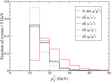
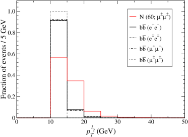
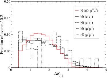
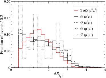
Figure 13: Distribution of several kinematical variables for $\mu^{\pm}\mu^{\pm}$ events from heavy neutrino production and dilepton events from $b\bar{b}$ production (see the text).

Finally, it is worth remarking here that raising the $p_{T}^{b}$ threshold at generator level, e.g. to 50 GeV, leads to a dramatic reduction of the $b\bar{b}nj$ cross sections, making the simulation more manageable. However, this also results in a gross underestimation of the $b\bar{b}nj$ background. We have checked this by simulating two samples of 25 million $b\bar{b}$ events with $p_{T}^{b}\geq 20$ and $p_{T}^{b}\geq 50$ GeV, respectively. For pre-selection we just require two isolated muons of either charge with $p_{T}^{\mu}\geq 10$ GeV. For the $p_{T}^{b}\geq 20$ sample we obtain 364 $b\bar{b}\to\mu\mu$ events, while for the $p_{T}^{b}\geq 50$ sample we only obtain 287 events. Given the difference in cross sections (1430 nb for $p_{T}^{b}\geq 20$ GeV and 58.8 nb for $p_{T}^{b}\geq 50$ GeV), raising $p_{T}^{b}$ to 50 GeV at event generation would underestimate this backgrounds by a factor of 30. For $b\bar{j}$ we have checked that raising $p_{T}^{b}$ at event generation to 50 GeV reduces the number of dimuon events by a factor of 35. This seems to be related to the fact that $b$ quarks with larger transverse momentum give more collimated decay products, and thus the muons are less isolated. On the other hand, $b$ quarks with too low transverse momentum cannot produce muons with $p_{T}^{\mu}\geq 10$ GeV. For this reason, we expect that our evaluation of $b\bar{b}nj$ provides a good estimate of the actual background to be found at LHC.

The evaluation of from $c\bar{c}nj$ proceeds in the same way. However, the number of dilepton events is much smaller and no $\mu^{\pm}\mu^{\pm}$ events appear in the samples simulated (containing about 145 million events after MLM matching). In this case the number of $\mu^{\pm}\mu^{\pm}jj$ events from $c\bar{c}nj$ production is estimated by comparing with $e^{\pm}e^{\pm}nj$ events and assuming the same ratio of events $N(\mu^{\pm}\mu^{\pm}jj)/N(e^{\pm}e^{\pm}jj)$ as for $b\bar{b}nj$ production. The result is shown between parentheses in the tables.

Appendix B Heavy neutrino mass reconstruction

For heavy neutrinos $N$ heavier than the $W$ boson the decay $N\to\mu W\to\mu q\bar{q}^{\prime}$ takes place with $W$ on shell; thus, the invariant mass of the two quarks is $M_{W}$ up to finite width effects. In simulated signal events, however, several extra jets often appear due to pile-up and initial/final state radiation, and it is not straightforward to identify the two ones originating from the $W$ decay. We have tested two procedures:

1. To take, naively, the two jets with highest transverse momentum. This method will be denoted as ‘R1’.

2. To try all possible pairings among the jets, choosing the pair giving an invariant mass closest to $M_{W}$. This method is denoted as ‘R2’.

The difference between the two choices is illustrated in Fig. 14 (left) for the case of the heavy neutrino signal. The method R1 yields a moderate peak for the $W$ reconstructed mass $M_{W}^{\text{rec}}$. When included in likelihood function (see Fig. 4), this variable improves the signal significance about 2%. (No improvement is found when performing a kinematical cut on $M_{W}^{\text{rec}}$ in addition to the cut on likelihood.) The second method R2 gives a considerably more peaked distribution for the signal, at the expense of strongly biasing the background, as it is shown in Fig. 14 (right). Thus, with the second method the $W$ invariant mass is not a useful variable for discriminating the signal against the background.

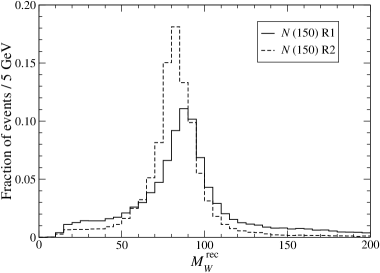
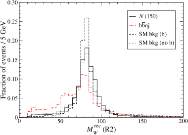
Figure 14: Left: reconstructed $W$ mass for the heavy neutrino signal, using the two methods (R1 and R2) explained in the text. Right: reconstructed $W$ mass for the signal and SM backgrounds using the method R2.

The heavy neutrino mass is obtained as the invariant mass of the jet pair selected to reconstruct the $W$, plus one of the two muons. In order to improve the reconstruction, the two jet momenta are rescaled so that their invariant mass coincides with $M_{W}$. For both $W$ reconstruction methods the results are very similar, as it can be observed in Fig. 15. The invariant mass of the $W$ and the muon with smaller transverse momentum $m_{W\mu_{2}}$ is more concentrated around the true $m_{N}$, and is taken as the heavy neutrino reconstructed mass in our analysis. In case of discovery, this distribution might be used to determine $m_{N}$.

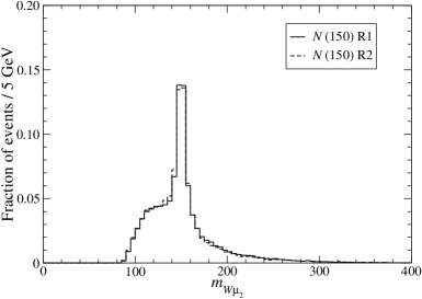
Figure 15: Invariant mass of the reconstructed $W$ boson (rescaled) and the muon with highest ($\mu_{1}$) and lowest ($\mu_{2}$) transverse momentum, for the two $W$ reconstruction choices explained in the text.

For $m_{N}<M_{W}$ it is very difficult to identify the two jets coming from $N\to W^{*}\mu$, which have low transverse momenta, due to the appearance of extra jets from pile-up. This fact is clearly seen examining the invariant mass distribution of the two jets with highest $p_{T}$ and either of the two muons, in Fig. 16. In both cases the distribution peaks well above $m_{N}=60$ GeV, indicating that one or the two jets do not really originate from the heavy neutrino decay. We have not found any improvement of the signal significance considering these variables in the likelihood analysis.

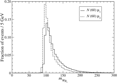
Figure 16: Invariant mass of the two jets with highest transverse momentum and each of the two muons, for a heavy neutrino signal with $m_{N}=60$ GeV.

In case of discovery, one possibility for the $N$ mass determination could be to consider the invariant mass of the two muons, which we present in Fig. 17 (left) for heavy neutrino masses of 50, 60 and 70 GeV. This distribution seems to peak around $m_{N}/2$. Other possibility is to exploit the fact that, since the on-shell decay $W\to\mu N$ is two-body, the energy of this muon in the centre of mass (CM) system, $E_{\mu}^{\text{CM}}$, is fixed by $m_{N}$. Thus, we may determine the heavy neutrino mass as

$$m_{N}^{\text{CM}}=\sqrt{M_{W}^{2}-2M_{W}E_{\mu}^{\text{CM}}}\,.$$ (14)

The $m_{N}$ reconstruction from the muon energy in the CM frame (defined as the rest frame of the two muons and two jets with largest $p_{T}$) is shown in Fig. 17 (right). For each event two values of $m_{N}^{\text{CM}}$ are calculated, corresponding to the two possible muon choices, and both are plotted. Imaginary values are discarded. These procedures for $m_{N}$ determination will be subject to possibly large systematic uncertainties, but their evaluation is beyond the scope of this work. (For example, the reconstruction from the muon energy in the CM frame is expected to have a systematic uncertainty from pile-up, which could be decreased using the muon energy in the laboratory frame, but at the expense of losing sensitivity to $m_{N}$.) If heavy neutrinos were discovered, interesting information about CP violation, relevant for leptogenesis, could also be inferred [42].

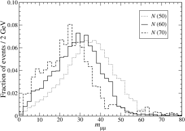
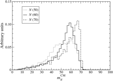
Figure 17: Left: invariant mass of the two muons, for three heavy neutrino masses. Right: heavy neutrino mass reconstructed from the muon energy in CM frame.

References

- [1] A. Datta, M. Guchait and A. Pilaftsis, Probing lepton number violation via Majorana neutrinos at hadron supercolliders, Phys. Rev. D 50 (1994) 3195 [hep-ph/9311257].
- [2] F. M. L. Almeida, Y. A. Coutinho, J. A. Martins Simoes and M. A. B. do Vale, On a signature for heavy Majorana neutrinos in hadronic collisions, Phys. Rev. D 62 (2000) 075004 [hep-ph/0002024].
- [3] O. Panella, M. Cannoni, C. Carimalo and Y. N. Srivastava, Signals of heavy Majorana neutrinos at hadron colliders, Phys. Rev. D 65 (2002) 035005 [hep-ph/0107308].
- [4] T. Han and B. Zhang, Signatures for Majorana neutrinos at hadron colliders, Phys. Rev. Lett. 97 (2006) 171804 [hep-ph/0604064].
- [5] F. del Aguila, J. A. Aguilar-Saavedra and R. Pittau, Neutrino physics at large colliders, J. Phys. Conf. Ser. 53 (2006) 506 [hep-ph/0606198].
- [6] P. Langacker, R. W. Robinett and J. L. Rosner, New heavy gauge bosons in and collisions, Phys. Rev. D 30 (1984) 1470.
- [7] A. Ferrari et al., Sensitivity study for new gauge bosons and right-handed Majorana neutrino in collisions at TeV, Phys. Rev. D 62 (2000) 013001.
- [8] S. N. Gninenko, M. M. Kirsanov, N. V. Krasnikov and V. A. Matveev, Detection of heavy Majorana neutrinos and right-handed bosons, CMS-NOTE-2006-098.
- [9] W. Y. Keung and G. Senjanovic, Majorana Neutrinos And The Production Of The Right-Handed Charged Gauge Boson, Phys. Rev. Lett. 50, 1427 (1983).
- [10] A. Datta, M. Guchait and D. P. Roy, Prospect of heavy right-handed neutrino search at SSC / LHC energies, Phys. Rev. D 47 (1993) 961 [hep-ph/9208228].
- [11] F. del Aguila and J. A. Aguilar-Saavedra, Like-sign dilepton signals from a leptophobic boson, arXiv:0705.4117 [hep-ph].
- [12] M. L. Mangano, M. Moretti, F. Piccinini, R. Pittau and A. D. Polosa, ALPGEN, a generator for hard multiparton processes in hadronic collisions, JHEP 0307 (2003) 001 [hep-ph/0206293].
- [13] R.N. Mohapatra and P.B. Pal, Massive neutrinos in physics and astrophysics: second edition, World Sci. Lect. Notes Phys. 72 (2004) 1.
- [14] G.C. Branco, L. Lavoura and J.P. Silva, CP Violation, Oxford University Press, Oxford, UK (1999).
- [15] J. Gluza and M. Zralek, Heavy neutrinos production and decay in future colliders, Phys. Rev. D 55 (1997) 7030 [hep-ph/9612227].
- [16] A. Pilaftsis, Radiatively induced neutrino masses and large Higgs neutrino couplings in the Standard Model with Majorana fields, Z. Phys. C 55 (1992) 275 [hep-ph/9901206].
- [17] F. del Aguila and J. A. Aguilar-Saavedra, production at CLIC: A window to TeV scale non-decoupled neutrinos, JHEP 0505 (2005) 026 [hep-ph/0503026].
- [18] S. Bergmann and A. Kagan, -induced FCNCs and their effects on neutrino oscillations, Nucl. Phys. B 538 (1999) 368 [hep-ph/9803305].
- [19] B. Bekman, J. Gluza, J. Holeczek, J. Syska and M. Zralek, Matter effects and CP violating neutrino oscillations with non-decoupling heavy neutrinos, Phys. Rev. D 66 (2002) 093004 [hep-ph/0207015].
- [20] C. Aalseth et al., Neutrinoless double beta decay and direct searches for neutrino mass, hep-ph/0412300.
- [21] P. Benes, A. Faessler, F. Simkovic and S. Kovalenko, Sterile neutrinos in neutrinoless double beta decay, Phys. Rev. D 71 (2005) 077901 [hep-ph/0501295].
- [22] G. Ingelman and J. Rathsman, Heavy Majorana neutrinos at colliders, Z. Phys. C 60 (1993) 243.
- [23] A. Ilakovac and A. Pilaftsis, Flavor violating charged lepton decays in seesaw-type models, Nucl. Phys. B 437 (1995) 491 [hep-ph/9403398].
- [24] D. Tommasini, G. Barenboim, J. Bernabeu and C. Jarlskog, Nondecoupling of heavy neutrinos and lepton flavor violation, Nucl. Phys. B 444 (1995) 451 [hep-ph/9503228].
- [25] F. del Aguila, J. A. Aguilar-Saavedra, A. Martinez de la Ossa and D. Meloni, Flavour and polarisation in heavy neutrino production at colliders, Phys. Lett. B 613 (2005) 170 [hep-ph/0502189].
- [26] E. Murayama, I. Watanabe and K. Hagiwara, HELAS: HELicity Amplitude Subroutines for Feynman Diagram Evaluations, KEK report 91-11, January 1992.
- [27] H. K. Dreiner, P. Richardson and M. H. Seymour, Resonant slepton production in hadron hadron collisions, Phys. Rev. D 63 (2001) 055008 [hep-ph/0007228].
- [28] A. Abulencia et al. [CDF Collaboration], Inclusive search for new physics with like-sign dilepton events in collisions at TeV, hep-ex/0702051.
- [29] T. Sjostrand, S. Mrenna and P. Skands, PYTHIA 6.4 physics and manual, JHEP 0605 (2006) 026 [hep-ph/0603175].
-
[30]
M. L. Mangano, talk at Lund University,
http://cern.ch/mlm/talks/lund-alpgen.pdf - [31] E. Richter-Was, D. Froidevaux and L. Poggioli, ATLFAST 2.0 a fast simulation package for ATLAS, ATLAS note ATL-PHYS-98-131.
- [32] O. Adriani et al. [L3 Collaboration], Search for isosinglet neutral heavy leptons In decays, Phys. Lett. B 295 (1992) 371.
- [33] P. Achard et al. [L3 Collaboration], Search for heavy isosinglet neutrino in annihilation at LEP, Phys. Lett. B 517 (2001) 67 [hep-ex/0107014].
- [34] D0 Collaboration, Search for the associated production of charginos and neutralinos in the like sign dimuon channel, note 5126-CONF.
- [35] G. J. Feldman and R. D. Cousins, A Unified approach to the classical statistical analysis of small signals, Phys. Rev. D 57 (1998) 3873 [physics/9711021].
- [36] G. Azuelos and A. Djouadi, New Fermions At Colliders. 2. Signals And Backgrounds, Z. Phys. C 63 (1994) 327 [hep-ph/9308340].
- [37] F. del Aguila, L. Ametller, G. L. Kane and J. Vidal, Vector-like fermion and standard Higgs production at hadron colliders,” Nucl. Phys. B 334 (1990) 1.
- [38] J. A. Aguilar-Saavedra, Light Higgs boson discovery from fermion mixing, JHEP 0612 (2006) 033 [hep-ph/0603200].
- [39] W. Porod, M. Hirsch, J. Romao and J. W. F. Valle, Testing neutrino mixing at future collider experiments, Phys. Rev. D 63 (2001) 115004 [hep-ph/0011248].
- [40] M. Hirsch and W. Porod, Neutrino properties and the decay of the lightest supersymmetric particle, Phys. Rev. D 68 (2003) 115007 [hep-ph/0307364].
- [41] R. Barate et al. [ALEPH Collaboration], Studies of quantum chromodynamics with the ALEPH detector, Phys. Rept. 294 (1998) 1.
- [42] S. Bray, J. S. Lee and A. Pilaftsis, Resonant CP violation due to heavy neutrinos at the LHC, hep-ph/0702294.