Elastic $pp$ and $\bar{p}p$ scattering
in the models of unitarized pomeron

E. Martynov Bogolyubov Institute for Theoretical Physics, 03680 Kiev, Ukraine.
e-mail: martynov@bitp.kiev.ua
Abstract

Elastic scattering amplitudes dominated by the Pomeron singularity which obey the principal unitarity bounds at high energies are constructed and analyzed. Confronting the models of double and triple (at $t=0$) Pomeron pole (supplemented by some terms responsible for the low energy behaviour) with existing experimental data on $pp$ and $\bar{p}p$ total and differential cross sections at $\sqrt{s}\geq 5$ GeV and $|t|\leq 6$ GeV2 we are able to tune the form of the Pomeron singularity. Actually the good agreement with those data is received for both models though the behaviour given by the dipole model is more preferable in some aspects. The predictions made for the LHC energy values display, however, the quite noticeable difference between the predictions of models at $t\approx-0.4$ GeV2. Apparently the future results of TOTEM will be more conclusive to make a true choice.

pacs:
13.85.Dz, 11.55.Jy, 13.60.Hb, 13.85.-t

I Introduction

The forthcoming TOTEM experiment at LHC will provide us, in fact, with the first measurements of soft pomeron (strictly speaking pomeron and odderon) as the contributions of secondary reggeons are negligible at such high energies. Then obviously the precise measurement of $pp$ differential cross section makes it possible to discriminate the various pomeron models comparing their particular predictions. Certainly, such an analysis makes sense only if the same data set is used with the model parameters reliably fixed. For the time being there are three model types for elastic hadron scattering amplitudes which reproduce rising cross sections experimentally measured with a high precision.

  • β€’

    Models treating Pomeron (and odderon as well) as a simple pole in a complex momentum plane located righter of unity, $\alpha_{P}(0)=1+\varepsilon\approx 1.1$ PVL ; DGP . In order to describe a dip-bump structure in differential cross section one should take into account the cuts in one or another form. Such a pomeron violates unitarity bound Οƒt​(s)≀C​l​n2​ssubscriptπœŽπ‘‘π‘ πΆπ‘™superscript𝑛2𝑠\sigma_{t}(s)\leq Cln^{2}s at sβ†’βˆžβ†’π‘ s\to\infty. However, the argument that unitarity corrections are important only at higher energies justifies this approach.

  • β€’

    Pomeron with $\alpha_{P}(0)>1$ is an input in some scheme of unitarization (for example, eikonal or quasieikonal eik , $U$-matrix models UM ). Having done the unitarization all such models give Οƒt​(s)∝l​n2​sproportional-tosubscriptπœŽπ‘‘π‘ π‘™superscript𝑛2𝑠\sigma_{t}(s)\propto ln^{2}{s}, whereas other characteristic predictions depend on the concrete model.

  • β€’

    Another way to construct amplitude is just to take into account unitarity and analytical requirements from the beginning as well as experimental information on the cross sections (e.g. growth of total cross sections). Such a model we named in what follows as model of unitarized pomeron. Here most successful examples are tripole pomeron (Οƒt​(s)∝l​n2​sproportional-tosubscriptπœŽπ‘‘π‘ π‘™superscript𝑛2𝑠\sigma_{t}(s)\propto ln^{2}s) LNGLN ; GLN ; AGN and dipole pomeron (Οƒt​(s)∝l​n​sproportional-tosubscriptπœŽπ‘‘π‘ π‘™π‘›π‘ \sigma_{t}(s)\propto lns) JMS ; DGMP .

Within the third approach we consider the models of tripole and dipole pomeron. These models are most successful in a description of all data on the forward scattering data COMPETE .

As it was shown COMPETE ; DGMP2 the total cross sections of meson and nucleon interactions are described with the minimal $\chi^{2}$ in the dipole and tripole models in which forward scattering amplitudes are parameterized in explicit analytic form. This conclusion was confirmed by analysis applying the dispersion relations for real part of amplitudes clms-disp .

The elastic scattering at small-$|t|$ ($0.1\leq|t|\leq 0.5$ GeV2) ($pp,\bar{p}p,\pi^{\pm}p$ and $K^{\pm}p$) was analyzed in detail CLM . The particular model was considered as a combination of hard (with $\alpha_{h}(0)\approx 1.4$) and soft $\alpha_{s}(0)\approx 1.1$ pomeron contributions. It was noticed in CLMS that additional hard pomeron essentially improves the description of the meson and nucleon data on parameter ρ=β„œβ‘e​A​(s,0)/ℑ⁑m​A​(s,0)πœŒπ‘’π΄π‘ 0π‘šπ΄π‘ 0\rho=\Re eA(s,0)/\Im mA(s,0) comparing with ordinary soft pomeron model. Extension of the model to higher $|t|$ can be done within some scheme of unitarization (e.g. eikonal, quasieikonal, $U-matrix$) taking into account pomeron rescatterings or cuts.

Here we focus on the dipole and tripole pomeron models. Without entering the details we note here these models describe the small-$|t|$ differential cross sections with the same level of precision ($\chi^{2}/dof\lesssim 1.05$, dof$\equiv$ degrees of freedom) as the model of CLM did. The purpose of the present paper is to demonstrate the description of the data on elastic $pp$ and $\bar{p}p$ scattering at low and middle $t$ in the dipole and tripole pomeron models.

In Sec. II we remind the general restrictions on hardness of pomeron singularity and form of its trajectory at small $t$, imposed by unitarity bounds on cross sections. In Sec. III and in Sec. IV parametrizations of $pp$ and $\bar{p}p$ elastic scattering amplitudes are presented dealing with dipole and tripole pomeron models, correspondingly. Results of least square analysis for both models as well as their comparison are given in the Sec. V.

II General constraints

Let us reiterate here that the model with Οƒt​(s)∝l​n2​sproportional-tosubscriptπœŽπ‘‘π‘ π‘™superscript𝑛2𝑠\sigma_{t}(s)\propto ln^{2}s is not compatible with a linear pomeron trajectory having the intercept 1. Indeed, let us assume that

$$\alpha_{P}(t)=1+\alpha_{P}^{\prime}t$$

and the partial wave amplitude develops the form

$$\varphi(j,t)=\eta(j)\frac{\beta(j,t)}{\left[j-1-\alpha_{P}^{\prime}t\right]^{n}}\approx\frac{i\beta(1,t)}{\left[j-1-\alpha_{P}^{\prime}t\right]^{n}},$$ (1)
$$\eta(j)=\frac{1+e^{-i\pi j}}{-\sin\pi j}.$$

In ($s,t$)-representation amplitude $\varphi(j,t)$ is transformed to

a​(s,t)=12​π​iβ€‹βˆ«π‘‘j​φ​(j,t)​eξ​(jβˆ’1),ΞΎ=l​n​(s/s0).formulae-sequenceπ‘Žπ‘ π‘‘12πœ‹π‘–differential-dπ‘—πœ‘π‘—π‘‘superscriptπ‘’πœ‰π‘—1πœ‰π‘™π‘›π‘ subscript𝑠0a(s,t)=\frac{1}{2\pi i}\int dj\varphi(j,t)e^{\xi(j-1)},\quad\xi=ln(s/s_{0}). (2)

Then, we have pomeron contribution at large $s$ as

a​(s,t)β‰ˆβˆ’g​(t)​[l​n​(βˆ’i​s/s0)]nβˆ’1​(βˆ’i​s/s0)Ξ±P′​tπ‘Žπ‘ π‘‘π‘”π‘‘superscriptdelimited-[]𝑙𝑛𝑖𝑠subscript𝑠0𝑛1superscript𝑖𝑠subscript𝑠0subscriptsuperscript𝛼′𝑃𝑑a(s,t)\approx-g(t)[ln(-is/s_{0})]^{n-1}(-is/s_{0})^{\alpha^{\prime}_{P}t} (3)

where

g​(t)=β​(t)/s​i​n​(π​αP​(t)/2).π‘”π‘‘π›½π‘‘π‘ π‘–π‘›πœ‹subscript𝛼𝑃𝑑2g(t)=\beta(t)/\\ sin(\pi\alpha_{P}(t)/2).

If as usually $g(t)=g\exp(bt)$ then we obtain

Οƒt​(s)subscriptπœŽπ‘‘π‘ \displaystyle\sigma_{t}(s) $\displaystyle\propto ln^{n-1}s,$
Οƒe​l​(s)subscriptπœŽπ‘’π‘™π‘ \displaystyle\sigma_{el}(s) ∝1s2β€‹βˆ«βˆ’βˆž0𝑑t​|a​(s,t)|2∝l​n2​nβˆ’3​s.proportional-toabsent1superscript𝑠2superscriptsubscript0differential-d𝑑superscriptπ‘Žπ‘ π‘‘2proportional-to𝑙superscript𝑛2𝑛3𝑠\displaystyle\propto\frac{1}{s^{2}}\int\limits_{-\infty}^{0}dt|a(s,t)|^{2}\propto ln^{2n-3}s. (4)

According to the obvious inequality,

Οƒe​l​(s)≀σt​(s)subscriptπœŽπ‘’π‘™π‘ subscriptπœŽπ‘‘π‘ \sigma_{el}(s)\leq\sigma_{t}(s) (5)

we have

$$2n-3\leq n-1\qquad\Rightarrow\qquad n\leq 2.$$ (6)

Thus we come to the conclusion that a model with Οƒt​(s)∝l​n2​sproportional-tosubscriptπœŽπ‘‘π‘ π‘™superscript𝑛2𝑠\sigma_{t}(s)\propto ln^{2}s is incompatible with a linear pomeron trajectory. In other words the partial amplitude Eq. (1) with $n=3$ (but used in some papers) in principle is incorrect.

If $n=1$ we have a simple $j$-pole leading to constant total cross section and vanishing elastic cross section. However such a behaviour of the cross sections is not supported by experimental data.

If $n=2$ we have the model of dipole pomeron (Οƒt​(s)∝l​n​(s)proportional-tosubscriptπœŽπ‘‘π‘ π‘™π‘›π‘ \sigma_{t}(s)\propto ln(s)) and would like to emphasize that double $j$-pole is the maximal singularity of partial amplitude settled by unitarity bound (5) if its trajectory is linear at $t\approx 0$.

Thus, constructing the model leading to cross section which increases faster than $ln(s)$, we need to consider a more complicated case:

$$\varphi(j,t)=\eta(j)\frac{\beta(j,t)}{\left[j-1+k(-t)^{1/\mu}\right]^{n}}\approx\frac{i\beta(1,t)}{\left[j-1+k(-t)^{1/\mu}\right]^{n}}.$$ (7)

Making use of the same arguments as above, we obtain

Οƒt​(s)∝l​nnβˆ’1​s,proportional-tosubscriptπœŽπ‘‘π‘ π‘™superscript𝑛𝑛1𝑠\sigma_{t}(s)\propto ln^{n-1}s, (8)
Οƒe​l​(s)∝l​n2​nβˆ’2βˆ’ΞΌβ€‹sandΞΌβ‰₯nβˆ’1.formulae-sequenceproportional-tosubscriptπœŽπ‘’π‘™π‘ π‘™superscript𝑛2𝑛2πœ‡π‘ andπœ‡π‘›1\sigma_{el}(s)\propto ln^{2n-2-\mu}s\qquad\mbox{and}\qquad\mu\geq n-1.

However in this case amplitude a​(s,t)π‘Žπ‘ π‘‘a(s,t) has a branch point at $t=0$ which is forbidden by analyticity.

A proper form of amplitude leading to $t_{eff}$ 111$t_{eff}$ can be defined by behaviour of elastic scattering amplitude at sβ†’βˆžβ†’π‘ s\to\infty. If a​(s,t)β‰ˆs​f​(s)​F​(t/te​f​f​(s))π‘Žπ‘ π‘‘π‘ π‘“π‘ πΉπ‘‘subscript𝑑𝑒𝑓𝑓𝑠a(s,t)\approx sf(s)F(t/t_{eff}(s)) then Οƒe​l​(s)∝|f​(s)|2β€‹βˆ«βˆ’βˆž0𝑑t​|F​(t/te​f​f)|2=te​f​f​|f​(s)​F​(1)|2proportional-tosubscriptπœŽπ‘’π‘™π‘ superscript𝑓𝑠2superscriptsubscript0differential-d𝑑superscript𝐹𝑑subscript𝑑𝑒𝑓𝑓2subscript𝑑𝑒𝑓𝑓superscript𝑓𝑠𝐹12\sigma_{el}(s)\propto|f(s)|^{2}\int_{-\infty}^{0}dt|F(t/t_{eff})|^{2}=t_{eff}|f(s)F(1)|^{2}. decreasing faster than $1/lns$ (it is necessary for $\sigma_{t}$ rising faster than $lns$) is the following

$$\varphi(j,t)=\eta(j)\frac{\beta(j,t)}{\left[(j-1)^{m}-kt\right]^{n}}.$$ (9)

Now we have $m$ branch points colliding at $t=0$ in $j$-plane and creating the pole of order $mn$ at $j=1$ (but there is no branch point in $t$ at $t=0$). At the same time te​f​f∝1/l​nm​sproportional-tosubscript𝑑𝑒𝑓𝑓1𝑙superscriptπ‘›π‘šπ‘ t_{eff}\propto 1/ln^{m}s and from the Οƒe​l∝l​n2​m​nβˆ’2βˆ’m​s≀σt∝l​nm​nβˆ’1​s≀l​n2​sproportional-tosubscriptπœŽπ‘’π‘™π‘™superscript𝑛2π‘šπ‘›2π‘šπ‘ subscriptπœŽπ‘‘proportional-to𝑙superscriptπ‘›π‘šπ‘›1𝑠𝑙superscript𝑛2𝑠\sigma_{el}\propto ln^{2mn-2-m}s\leq\sigma_{t}\propto ln^{mn-1}s\leq ln^{2}s one can obtain

$$\left\{\begin{array}[]{ll}mn&\leq m+1,\\ mn&\leq 3.\end{array}\right.$$ (10)

If $\sigma_{el}\propto\sigma_{t}$ then $n=1+\frac{1}{m}$. Furthermore, if Οƒt∝l​n​sproportional-tosubscriptπœŽπ‘‘π‘™π‘›π‘ \sigma_{t}\propto lns then $m=1$ and $n=2$ what corresponds just to the dipole pomeron model. In the tripole pomeron model $m=2$ and $n=3/2$ what means $\sigma_{t}\propto ln^{2}s$.

III Dipole parametrizations

The dominating term at high energy in this model is double pole

$$\varphi_{d}(j,t)\propto\frac{1}{(j-1-\alpha_{d}^{\prime}t)^{2}}.$$ (11)

Apparently in accordance with the inequalities (10) the double pole obeys the unitarity limit for linear pomeron trajectory ($m=1$). Adding to the partial amplitude less singular term (simple pole with a trajectory having intercept $\alpha(0)=1$ and a different slope $\alpha^{\prime}$) we obtain dipole pomeron model in the form

$$\varphi(j,t)=\eta(j)\frac{\beta_{d}(t)}{(j-1-\alpha_{d}^{\prime}t)^{2}}+\eta(j)\frac{\beta_{s}(t)}{j-1-\alpha_{s}^{\prime}t}.$$ (12)

It can be rewritten in $(s,t)$ representation as

a​(s,t)=π‘Žπ‘ π‘‘absent\displaystyle a(s,t)= $\displaystyle g_{d}ln(-iz)(-iz)^{1+\alpha_{d}^{\prime}t}\exp(b_{d}t)$ (13)
$\displaystyle+g_{s}(-iz)^{1+\alpha_{s}^{\prime}t}\exp(b_{s}t),$

where variable $z$ is proportional to cosine of scattering angle in $t$-channel

$$z=(t+2(s-2m_{p}^{2}))/z_{0},\qquad z_{0}=1{\rm GeV}^{2}.$$ (14)

Generally, the form factors (or residues) $\beta(t)$ may be chosen in various forms (e.g. exponential, factorized powers etc.). However we consider the simplest exponential ones.

Let us consider two effective reggeons: crossing-even, $R_{+}(s,t)$, and crossing-odd, $R_{-}(s,t)$) instead of four contributions - $f,\omega$ and $\rho,a_{2}$ (the latter two reggeons are of less importance at high energy). We take into account their contribution in the standard form. However, we insert additional factor $Z_{R}(t)$ that changes a sign at some $t$ 222For crossing-odd term of amplitude such a factor is well known and describes crossover effect, i.e. intersection of the $ab$ and $\bar{a}b$ differential cross sections at $t\approx-0.15$ GeV2. Our analysis CLM has shown that similar factor is visible in crossing-even reggeon term..

$$R(s,t)=\eta_{R}g_{R}Z_{R}(t)(-iz)^{\alpha_{R}(t)}\exp(b_{R}t),$$ (15)

where $\eta_{R}=-1/\sin(0.5\pi\alpha_{+}(0))$ for $R_{+}$-reggeon and $\eta_{R}=i/\cos(0.5\pi\alpha_{-}(0))$ for $R_{-}$-reggeon. Obviously these terms are very close to $f$- and $\omega$-reggeons, respectively. There are some arguments CLM to use the factors $Z_{R}(t)$ in the form:

$$Z_{R}(t)=\frac{\tanh(1+t/t_{R})}{\tanh(1)}.$$ (16)

Going to extend wide regions of $s$ ($\sqrt{s}\geq 5$ GeV) and $t$ ($0.1\leq|t|\leq 6$ GeV2) 333A more sophisticated form for residues should be considered for larger $|t|$. we certainly need a few extra terms in amplitude to reach a good fit to the data. First of all it concerns the odderon contribution. The existing data on total cross section and parameters ρ=β„œβ‘e​a​(s,0)/ℑ⁑m​a​(s,0)πœŒπ‘’π‘Žπ‘ 0π‘šπ‘Žπ‘ 0\rho=\Re ea(s,0)/\Im ma(s,0), as well known, do not show any visible odderon contribution. However, it appears definitely to provide the difference of $pp$ and $\bar{p}p$ differential cross sections at $\sqrt{s}=53$ GeV and $t$ around the dip. So, we add the odderon contribution vanishing at $t=0$

$\displaystyle{\cal O}(s,t)=t^{2}zZ_{R_{-}}(t)\biggl{\{}$ $\displaystyle\!\!\!o_{1}ln^{2}(-iz)\exp(b_{o1}t)$ (17)
$\displaystyle\!\!\!+o_{2}ln(-iz)\exp(b_{o2}t)$
$\displaystyle\!\!\!+o_{3}\exp(b_{o3}t)\biggr{\}}(-iz)^{1+\alpha_{o}^{\prime}t}$

The term $\propto ln^{2}(s)$ in Eq. 17 does not violate unitarity restriction Οƒe​l​(s)≀σt​(s)subscriptπœŽπ‘’π‘™π‘ subscriptπœŽπ‘‘π‘ \sigma_{el}(s)\leq\sigma_{t}(s) at very large $s$ due to presence of factor $t^{2}$ (in the dipole model $t_{eff}\sim 1/lns$, therefore $\sigma_{el}\propto t^{3}_{eff}ln^{4}s\propto lns$).

At high energy and at $t=0$ two main rescattering terms of dipole pomeron (or cut terms) have the same form as the input amplitude - double pole plus simple pole. It means that comparing the model with experimental data we are not able to distinguish unambiguously input terms and cuts. Then as result, at $t=0$ one may use the input amplitude only. At tβ‰ 0𝑑0t\neq 0 the situation occurs more complicated because the slopes of trajectories in the cut terms are different from the input one. These terms are important at large $|t|$ but, in fact, they are already taken into account at $t=0$.

Keeping in mind the above arguments and preserving a good description of the data at $t=0$ we take pomeron, pomeron-pomeron and pomeron-reggeons cuts vanishing at $t=0$. Certainly they are not ”genuine” rescatterings but mimic them quite efficiently at tβ‰ 0𝑑0t\neq 0. Thus we write down:

the pomeron contribution

$$P(s,t)=-g_{P}(-iz)^{1+\alpha_{P}^{\prime}t}\left[\exp(b_{P1}t)-\exp(b_{P2}t)\right],$$ (18)

the pomeron-pomeron cut

$$C_{P}(s,t)=-\frac{t}{ln(-iz)}g_{PP}(-iz)^{1+\alpha_{P}^{\prime}t/2}\exp(b_{PP}t),$$ (19)

the pomeron-even reggeon cut

$\displaystyle C_{R_{+}}(s,t)=$ $\displaystyle-\frac{tZ_{R_{+}}(t)}{ln(-iz)}\eta_{R_{+}}g_{P+}Z_{R_{+}}(t)$ (20)
$\displaystyle\times(-iz)^{\alpha_{+}(0)+\alpha^{\prime}_{P+}t}\exp(b_{P+}t),$

where

$$\alpha^{\prime}_{P+}=\frac{\alpha_{P}^{\prime}\alpha_{R_{+}}^{\prime}}{\alpha_{P}^{\prime}+\alpha_{R_{+}}^{\prime}},$$ (21)

and the pomeron-odd reggeon cut

$\displaystyle C_{R_{-}}(s,t)=$ $\displaystyle-i\frac{tZ_{R_{-}}(t)}{ln(-iz)}\eta_{R_{-}}g_{P-}Z_{R_{-}}(t)$ (22)
$\displaystyle\times(-iz)^{\alpha_{-}(0)+\alpha^{\prime}_{P-}t}\exp(b_{P-}t),$
$$\alpha^{\prime}_{P-}=\frac{\alpha_{P}^{\prime}\alpha_{R_{-}}^{\prime}}{\alpha_{P}^{\prime}+\alpha_{R_{-}}^{\prime}}.$$ (23)

IV Tripole pomeron model

As it follows from Eq.(10) for the dominating contribution in a tripole pomeron model with Οƒt​(s)∝l​n2​(s)proportional-tosubscriptπœŽπ‘‘π‘ π‘™superscript𝑛2𝑠\sigma_{t}(s)\propto ln^{2}(s), i.e. $n=2$, $m=3/2$, we should take

$$\varphi_{1}(j,t)=\eta(j)\frac{\beta_{1}(j,t)}{\left[(j-1)^{2}-kt\right]^{3/2}}.$$ (24)

It seems to be natural to write the subleading terms as the following

$$\varphi_{2}(j,t)=\eta(j)\frac{\beta_{2}(j,t)}{\left[(j-1)^{2}-kt\right]},$$ (25)
$$\varphi_{3}(j,t)=\eta(j)\frac{\beta_{3}(j,t)}{\left[(j-1)^{2}-kt\right]^{1/2}}.$$ (26)

Then the amplitude has a form

$$\varphi(j,t)=\varphi_{1}(j,t)+\varphi_{2}(j,t)+\varphi_{3}(j,t)+R(j,t),$$ (27)

where $R(j,t)$ means the contribution of other reggeons and possible cuts (which are important at low energies).

Taking into account that

$$\int\limits_{0}^{\infty}dxx^{\alpha-1}e^{-\omega x}\textit{J}_{\nu}(\omega_{0})=I_{\nu}^{\alpha}$$ (28)

where

$$\begin{array}[]{ll}{I_{\nu}^{\nu+1}=\frac{(2\omega_{0})^{\nu}}{\sqrt{\pi}}\frac{\Gamma(\nu+1/2)}{(\omega^{2}+\omega_{0}^{2})^{\nu+1/2}}},\\ \\ {I_{\nu}^{\nu+2}=2\omega\frac{(2\omega_{0})^{\nu}}{\sqrt{\pi}}\frac{\Gamma(\nu+3/2)}{(\omega^{2}+\omega_{0}^{2})^{\nu+3/2}}},\end{array}$$

one can find

$$\frac{1}{(\omega^{2}+\omega_{0}^{2})^{3/2}}=\frac{1}{2\omega_{0}}\int\limits_{0}^{\infty}dxxe^{-x\omega}J_{1}(\omega_{0}x),$$ (29)
$$\frac{1}{\omega^{2}+\omega_{0}^{2}}=\frac{1}{\omega_{0}}\int\limits_{0}^{\infty}dxe^{-x\omega}\sin(x\omega_{0})$$ (30)

and

$$\frac{1}{(\omega^{2}+\omega_{0}^{2})^{1/2}}=\int\limits_{0}^{\infty}dxe^{-x\omega}J_{0}(\omega_{0}x).$$ (31)

Thus tripole amplitude with the subleading terms can be presented as

$\displaystyle a_{tr}(s,t)=iz\biggl{\{}$ $\displaystyle g_{+1}\exp(b_{+1}t)ln(-iz)\frac{2J_{1}(\xi_{+}\tau_{+})}{\tau_{+}}$ (32)
$\displaystyle+g_{+2}\frac{\sin(\xi_{+}\tau_{+})}{\tau_{+}}\exp(b_{+2}t)$
$\displaystyle+g_{+3}J_{0}(\xi_{+}\tau_{+})\exp(b_{+3}t)\biggr{\}}$

where $\xi_{+}=ln(-iz)+\lambda_{+}$, $z$ is defined by Exp.(14), and $\tau_{+}=r_{+}\sqrt{-t/t_{0}}$, $t_{0}=1$ GeV2, $r_{+}$ is a constant.

Similar expression for odderon contribution (but introducing the factors $t$ and $Z_{R_{-}}(t)$) is given by

$\displaystyle{\cal O}(s,t)=ztZ_{R_{-}}(t)\biggl{\{}$ $\displaystyle g_{-1}ln(-iz)\frac{2J_{1}(\xi_{-}\tau_{-})}{\tau_{-}}\exp(b_{-1}t)$ (33)
$\displaystyle+g_{-2}\frac{\sin(\xi_{-}\tau_{-})}{\tau_{-}}\exp(b_{-2}t)$
$\displaystyle+g_{-3}J_{0}(\xi_{-}\tau_{-})\exp(b_{-3}t)\biggr{\}}$

where $\xi_{-}=ln(-iz)+\lambda_{-}$ and $\tau_{-}=r_{-}\sqrt{-t/t_{0}}$.

Again, similarly to the dipole model we add the β€œsoft” pomeron

$$P(s,t)=-g_{P}(-iz)^{1+\alpha_{P}^{\prime}t}\exp(b_{P}t),$$ (34)

the reggeon and cut contributions which are of the same form as in dipole pomeron model Eqs.(19,20,22).

AGLN-model. Let us give a few comments about another version of tripole pomeron model presented in the papers GLN ; AGN .

1. If ΞΎ=l​n​(βˆ’i​s/s0),s0=1​G​e​V2formulae-sequenceπœ‰π‘™π‘›π‘–π‘ subscript𝑠0subscript𝑠01GesuperscriptV2\xi=ln(-is/s_{0}),s_{0}=1{\rm GeV}^{2}, then the first pomeron term in GLN ; AGN is identical to the term in Eq. (32) while for the second and third terms authors use

$$g_{2}(t)\xi J_{0}(\xi\tau)$$

and

$$g_{3}(t)[J_{0}(\xi\tau_{+})-\xi_{0}\tau_{+}J_{1}(\xi\tau_{+})]$$

which originated from the partial amplitudes

$$\varphi(j,t)=\eta(j)g_{2}(t)\frac{2(j-1)}{\left[(j-1)^{2}-kt\right]^{3/2}},$$

and

$$\varphi(j,t)=\eta(j)g_{2}(t)\frac{(j-1)^{2}+kt}{\left[(j-1)^{2}-kt\right]^{3/2}},$$

respectively.

2. They used another form of odderon terms. The maximal odderon contribution in the form

π’ͺm​(s,t)subscriptπ’ͺπ‘šπ‘ π‘‘\displaystyle{\cal O}_{m}(s,t) $\displaystyle=g_{-1}ln^{2}(-iz)\frac{\sin(\xi\tau_{-})}{\tau_{-}}\exp(b_{-1}t)$ (35)
$\displaystyle+g_{-2}ln(-iz)\cos(\xi\tau_{-})\exp(b_{-2}t)$
$\displaystyle+g_{-3}\exp(b_{-3}t)$

as well as a simple pole odderon and odderon-pomeron cut are also taken into account.

3. Omitting the details we note that because of the chosen form of signature factors the AGLN amplitude has pole in physical region at $t=-1/\alpha^{\prime}=-4$ GeV2. This feature of the model restricts its applicability region. AGLN amplitude has similar poles even at lower values of $|t|$ in the reggeon terms. Thus the model requires a modification to describe wider region of $t$ than was considered in AGN , namely $|t|\leq 2.6$ GeV2.

4. Clearly this model leads to the unreasonable intercept value for the crossing-odd reggeon, $\alpha_{-}(0)=0.34$. It is in strong contradiction with the values known from meson resonance spectroscopy data. One could expect it close to the intercept of $\omega$-trajectory, $\alpha_{\omega}(0)\approx 0.43-0.46$ DGMP2 .

Nevertheless, in the Section V we demonstrate the curves for differential cross sections obtained in AGLN model in comparison with the results of our dipole and tripole models at energies available and future LHC.

V Comparison with experimental data

V.1 Total cross sections

Analyzing the $pp$ and $\bar{p}p$ data we keep in mind a further extension of the models to elastic $\pi^{\pm}p$ and $K\pm p$ scattering, which are quite precisely measured. One important point should be underlined from the beginning. Fitting the $pp$ and $\bar{p}p$ data on $\sigma_{t}$ and $\rho$ gives the set of parameters which is essentially different from those derived from the fit of all ($p,\bar{p},\pi$- and $K$-meson) the data.

Following this procedure at the first stage we determine all parameters which control the amplitudes at $t=0$. We use the standard data set for the $\pi^{\pm}p$ and $K\pm p$ total cross sections and the ratios $\rho$ (at 5 GeV$\leq\sqrt{s}<$2000 GeV) PDG to find intercepts of $C_{\pm}$-reggeons and couplings of the reggeon and pomeron exchanges. There are 542 experimental points in the region under consideration (see Table 1).

An extension of the $pp\rightarrow pp$ and $\bar{p}p\rightarrow\bar{p}p$ dipole and tripole amplitudes to $\pi^{\pm}p$ and $K^{\pm}p$ elastic scattering is quite straight forward. All the couplings are various in these amplitudes at $t=0$ but the odderon does not contribute to the $\pi p$ and $Kp$ amplitudes. In the simplest unitarization schemes (eikonal, $U$-matrix) all total cross sections at asymptotically high energies have the universal behaviour, Οƒt​(s)β†’Οƒ0​log2⁑(sa​p/s0)β†’subscriptπœŽπ‘‘π‘ subscript𝜎0superscript2subscriptπ‘ π‘Žπ‘subscript𝑠0\sigma_{t}(s)\to\sigma_{0}\log^{2}(s_{ap}/s_{0}), where $\sigma_{0}$ is independent of the initial particles. Today the data available support this conclusion and advocates putting the same couplings $g_{+1}^{p}=g_{+1}^{\pi}=g_{+1}^{K}$ for the leading pomeron terms in all amplitudes. Besides, in order to avoid uncertainty at $t=0$ (constant contributions to total cross sections come additively from the third term of Eq.(32) and from β€œsoft” pomeron, Eq.(34)) we substitute couplings $g_{+3}$ for $g_{+3}-g_{P}$ in Eq.(32). As a result we have energy independent contribution to the total cross from $g_{+3}$ only.

The following normalization of $ab\rightarrow ab$ amplitude is used

Οƒt=1sa​b​ℑ⁑m​A​(s,0),d​σd​t=116​π​sa​b2​|A​(s,t)|2formulae-sequencesubscriptπœŽπ‘‘1subscriptπ‘ π‘Žπ‘π‘šπ΄π‘ 0π‘‘πœŽπ‘‘π‘‘116πœ‹superscriptsubscriptπ‘ π‘Žπ‘2superscript𝐴𝑠𝑑2\sigma_{t}=\frac{1}{s_{ab}}\Im mA(s,0),\qquad\frac{d\sigma}{dt}=\frac{1}{16\pi s_{ab}^{2}}|A(s,t)|^{2} (36)

where

sa​b=(sβˆ’ma2βˆ’mb2)2βˆ’4​ma2​mb2=2​pal​a​b​ssubscriptπ‘ π‘Žπ‘superscript𝑠superscriptsubscriptπ‘šπ‘Ž2superscriptsubscriptπ‘šπ‘224superscriptsubscriptπ‘šπ‘Ž2superscriptsubscriptπ‘šπ‘22superscriptsubscriptπ‘π‘Žπ‘™π‘Žπ‘π‘ s_{ab}=\sqrt{(s-m_{a}^{2}-m_{b}^{2})^{2}-4m_{a}^{2}m_{b}^{2}}=2p_{a}^{lab}\sqrt{s}

and $p_{a}^{lab}$ is the momentum of hadron $a$ in laboratory system of $b$.

The details of the fit at $t=0$ are presented in the Tables 1 and 2.

Table 1: Quality of the fit to $\sigma_{t}$ and $\rho$
$\chi^{2}_{tot}/N_{p}$
quantity number of data Dipole model Tripole model
$\sigma_{t}^{pp}$ 104 0.88260E+00 0.87055E+00
$\sigma_{t}^{\bar{p}p}$ 59 0.95280E+00 0.96273E+00
$\sigma_{t}^{\pi^{+}p}$ 50 0.66216E+00 0.66792E+00
$\sigma_{t}^{\pi^{-}p}$ 95 0.10023E+01 0.99864E+00
$\sigma_{t}^{K^{+}p}$ 40 0.72357E+00 0.72104E+00
$\sigma_{t}^{K^{-}p}$ 63 0.61392E+00 0.60883E+00
$\rho^{pp}$ 64 0.16612E+01 0.16965E+01
$\rho^{\bar{p}p}$ 11 0.40392E+00 0.40675E+00
$\rho^{\pi^{+}p}$ 8 0.15107E+01 0.15036E+01
$\rho^{\pi^{-}p}$ 30 0.12560E+01 0.12122E+01
$\rho^{K^{+}p}$ 10 0.10869E+01 0.10016E+01
$\rho^{K^{-}p}$ 8 0.12185E+01 0.11611E+01
$\chi^{2}_{tot}/dof$
Total 542 0.99450E+00 0.99345E+00
Table 2: Intercepts and couplings (GeV-2) in the Dipole and Tripole models from the fit to $\sigma_{t}$ and $\rho$
Dipole model Tripole model
parameter value error parameter value error
$\alpha_{R+}(0)$ 0.80846E+00 0.36035E-02 $\alpha_{R+}(0)$ 0.71947E+00 0.18496E-02
$\alpha_{R-}(0)$ 0.46505E+00 0.91416E-02 $\alpha_{R-}(0)$ 0.46356E+00 0.73746E-02
$g_{d}^{p}$ 0.89435E+01 0.19499E+00 $g_{+1}^{p}$ 0.15330E+02 0.31619E+00
$g_{s}^{p}$ -0.52159E+02 0.30078E+01 $g_{+2}^{p}$ 0.19153E+01 0.38589E-01
$g_{R+}^{p}$ 0.15857E+03 0.30846E+01 $g_{+3}^{p}$ 0.20672E+00 0.26747E-02
$g_{R-}^{p}$ 0.58961E+02 0.28775E+01 $g_{R+}^{p}$ 0.96906E+02 0.84678E+00
$g_{d}^{\pi}$ 0.70477E+01 0.22719E+00 $g_{R-}^{p}$ 0.59294E+02 0.23228E+01
gsΟ€superscriptsubscriptπ‘”π‘ πœ‹g_{s}^{\pi} -0.45720E+02 0.29022E+01 $g_{+1}^{\pi}$ 0.69901E+01 0.18396E+00
$g_{R+}^{\pi}$ 0.10691E+03 0.33590E+01 $g_{+2}^{\pi}$ 0.10106E+01 0.27123E-01
$g_{R-}^{\pi}$ 0.10710E+02 0.52507E+00 $g_{R+}^{\pi}$ 0.56296E+02 0.45360E+00
$g_{d}^{K}$ 0.54351E+01 0.29205E+00 $g_{R-}^{\pi}$ 0.10784E+02 0.43687E+00
$g_{s}^{K}$ -0.29703E+02 0.33234E+01 $g_{+1}^{K}$ 0.12186E+02 0.22424E+00
$g_{R+}^{K}$ 0.70785E+02 0.43792E+01 $g_{+2}^{K}$ 0.14683E+00 0.30439E-01
$g_{R-}^{K}$ 0.23674E+02 0.11159E+01 $g_{R+}^{K}$ 0.28730E+02 0.51047E+00
$g_{R-}^{K}$ 0.23831E+02 0.91697E+00

V.2 Differential cross sections

At the second stage of the fitting procedure we fix all the intercept and coupling values obtained at the first stage. The other parameters are determined by fitting the $d\sigma/dt$ data in the region

$$0.1{\rm GeV}^{2}\leq|t|\leq 6{\rm GeV}^{2},\quad\sqrt{s}\geq 5{\rm GeV}.$$ (37)

The measurements of the differential elastic cross sections were very intensive for the last 40 years. Fortunately, most of them have been collected in the Durham Data Base DDB . However, there are 80 papers, with different conventions, and various units. The complete list of the references is given by CLM . We have uniformly formatted them, found and corrected some errors in the sets and gave a detailed description of a full set which contains about 10000 points. Analyzing each subset of these data we have payed CLM particular attention to the data at small $t$. Some of subsets which are in strong disagreement with the rest of the dataset were excluded from the fit.

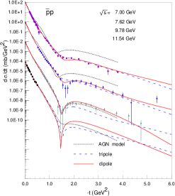
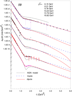
A similar work has been done for the data at $|t|>0.7$ GeV2. We have found out and corrected some mistakes in the data base. Furtermore, we excluded from the final dataset the subsets BRUNETON at $\sqrt{s}=9.235$ GeV, CONETTI at $\sqrt{s}=19.47$ and $27.43$ GeV from $pp$ data and BOGOLYUBSKY at $\sqrt{s}=7.875$ GeV, AKERLOF at $\sqrt{s}=9.778$ GeV from $\bar{p}p$ data because they strongly contradict the bulk of data. Thus, the considered models were fitted to 2532 points of $d\sigma/dt$ in the region Eq.(37). The results are given in the Table 3 for a quality of fitting and in the Table 4 for the fitting parameters.

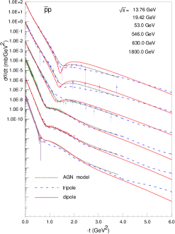
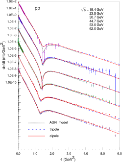
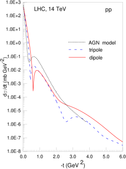
In the Figs. 1 - 5 we show experimental data at some energies and theoretical curves obtained in three models: AGLN AGN , Dipole and Tripole. As to the AGLN model, we would like to emphasize that the corresponding curves were calculated at the parameters given in AGN . However, in contrast to Dipole and Tripole models AGLN model was fitted to differential cross sections at $\sqrt{s}>9.7$ GeV and $|t|<2.6$ GeV2 but not with a complete dataset. Therefore a disagreement between curves and data behaviours at lowest energies is not surprising in the given model. The AGLN model works well at high energies.

Refer to caption
Figure 1: $\bar{p}p$ at low energies
Refer to caption
Figure 2: $pp$ at low energies
Refer to caption
Figure 3: $\bar{p}p$ at high energies
Refer to caption
Figure 4: $pp$ at high energies
Refer to caption
Figure 5: Predictions for LHC energy
Table 3: Quality of the fit to $d\sigma/dt$
Number of $\chi^{2}_{tot}/N_{p}$
points, $N_{p}$ Dipole model Tripole model
$d\sigma^{pp}/dt$ 1857 0.15122E+01 0.18153E+01
$d\sigma^{\bar{p}p}/dt$ 675 0.14183E+01 0.16697E+01
Table 4: Parameters of the models, from the fit to $d\sigma/dt$ (parameters $r_{\pm},\lambda_{\pm}$ are dimensionless, $t_{R\pm}$ are given in GeV2, the rest parameters are given in GeV-2).
Dipole model Tripole model
parameter value error parameter value error
$\alpha_{d}^{\prime}$ 0.30631E+00 0.16923E-02 $r_{+}$ 0.25417E+00 0.33181E-02
$\alpha_{s}^{\prime}$ 0.28069E+00 0.19026E-03 $\lambda_{+}$ 0.11575E+01 0.14824E+00
$b_{d}$ 0.38675E+01 0.22767E-01 $b_{+1}$ 0.34583E+01 0.37982E-01
$b_{s}$ 0.55679E+00 0.14694E-02 $b_{+2}$ 0.19091E+01 0.30598E-01
$\alpha_{R+}^{\prime}$ 0.82000E+00 fixed $b_{+3}$ 0.45970E+00 0.29750E-02
$b_{R+}$ 0.29226E+01 0.30019E-01 $\alpha_{R+}^{\prime}$ 0.82000E+00 fixed
$t_{R+}$ 0.48852E+00 0.26683E-02 $b_{R+}$ 0.10668E+01 0.30350E-01
$\alpha_{R-}^{\prime}$ 0.91000E+00 fixed $t_{R+}$ 0.54237E+00 0.13817E-01
$b_{R-}$ 0.15201E+01 0.68671E-01 $\alpha_{R-}^{\prime}$ 0.91000E+00 fixed
$t_{R-}$ 0.14497E+00 0.24811E-02 $b_{R-}$ 0.61435E-01 0.20044E-01
$o_{1}$ 0.30738E+00 0.31368E-02 $t_{R-}$ 0.15755E+00 0.26068E-02
$o_{2}$ -0.63119E+01 0.55282E-01 $r_{-}$ 0.78807E-01 0.60563E-02
$o_{3}$ 0.13456E+00 0.21551E-02 $\lambda_{-}$ 0.16281E+02 0.19020E+01
$\alpha_{o}^{\prime}$ 0.21810E-01 0.70324E-03 $o_{1}$ -0.56075E-01 0.51702E-02
$b_{o1}$ 0.39317E+01 0.81697E-02 $o_{2}$ 0.17372E+01 0.17893E+00
$b_{o2}$ 0.45007E+01 0.76861E-02 $o_{3}$ -0.61193E+02 0.36330E+01
$b_{o3}$ 0.12947E+01 0.76773E-02 $b_{o1}$ 0.12038E+01 0.26425E-01
$g_{P}$ 0.58961E+02 0.98576E-01 $b_{o2}$ 0.15152E+01 0.31722E-01
$\alpha_{P}^{\prime}$ 0.30696E+00 0.20475E-03 $b_{o3}$ 0.26331E+01 0.78349E-01
$b_{P1}$ 0.54894E+00 0.15036E-02 $g_{P}$ 0.16042E+02 13856E-01
$b_{P2}$ 0.59365E+01 0.34863E-01 $\alpha_{P}^{\prime}$ 0.36060E+00 0.76335E-02
$g_{PP}$ -0.39324E+02 0.36883E+00 $b_{P}$ 0.14662E+01 0.29152E-01
$b_{PP}$ 0.11828E+01 0.44025E-02 $g_{PP}$ 0.91195E+01 0.84044E+00
$g_{P+}$ -0.22656E+03 0.27529E+01 $b_{PP}$ 0.44977E+00 0.46404E-01
$b_{P+}$ 0.17522E+01 0.98459E-02 $g_{P+}$ 0.11772E+02 0.57753E+00
$g_{P-}$ -0.15255E+02 0.28213E+00 $b_{P+}$ 0.81585E-01 0.28185E-01
$b_{P-}$ 0.24068E-01 0.61336E-02 $g_{P-}$ 0.81908E+01 0.88408E+00
$b_{P-}$ -0.79115E-01 0.45833E-01

VI Conclusion

In this paper we compare three unitarized models of elastic scattering amplitude fitting the Dipole and Tripole models to all existing data. We emphasize that the amplitude leading to the behaviour of $\sigma_{t}\propto\ln^{2}s$ should be parameterized with a special care of the unitarity and analyticity restrictions on properties of the leading partial wave singularity.

The Figures and Tables demonstrate good description of the data within the considered models. However the obtained $\chi^{2}$ (Table 3) hints that the Dipole pomeron model looks more preferable.

We believe the most interesting and instructive result for further search of more realistic model is shown in Fig.Β 5. Our predictions of the compared models (together with AGLN model) for $pp$ cross section at LHC energy are crucially different at $|t|$ around 0.3 - 0.5 GeV2. Certainly the future TOTEM measurement will allow to distinguish between three considered models.

I would like to thank Prof.Β B.Β Nicolescu and Dr.Β J.R.Β Cudell for many useful discussions.

The work was supported partially by the Ukrainian Fund of Fundamental Researches.

References

  • (1) A. Donnachie and P.V. Landshoff, Phys. Lett. B296 227 (1992) ; P.V. Landshoff, arXiv:hep-ph/0509240; Nucl. Phys. Proc. Suppl. A99 311 (2001), [arXiv:hep-ph/0010315] and references therein.
  • (2) M. Giffon, P. Desgrolard and E. Predazzi, Z. Phys. C63 241 (1994).
  • (3) Discussion of an eikonal approximation in the Regge theory as well as references to the original papers on this subject can be found in P.D.B. Collins, An introduction to Regge theory & high energy physics, Cambridge University press (Cambridge) 1977;
    See also: K.A. Ter-Martirosyan, Sov. ZhETF Pisma 15 519 (1972);
    V.A. Petrov and A.V. Prokudin, Eur. Phys. J. C23 135 (2002);
    C.Β Bourrely, J.Β Soffer and T.T.Β Wu, Eur. Phys. J. C 28 97 (2003) [arXiv:hep-ph/0210264];
    P.A.S.Β Carvalho, A.F.Β Martini and M.J.Β Menon, Eur. Phys. J. C39 359 (2005) [arXiv:hep-ph/0312243].
  • (4) S.M. Troshin and N.E. Tyurin, Phys. Part. Nucl. 35 555 (2004); Fiz. Elem. Chast. Atom. Yadra 35 1029 (2004); [arXiv:hep-ph/0308027] and references therein;
    L.L. Jenkovszky, B.V. Struminsky and A.N. Wall, Sov. Journ. Part. Nucl. 19 180 (1988).
  • (5) L. Lukaszuk and B. Nicolescu, Nuovo Cimento Letters 8 405 1973;
    P. Gauron, E. Leader and B. Nicolescu, Nuclear Physics B299 640 (1988).
  • (6) P. Gauron, E. Leader and B. Nicolescu, Phys. Lett. B238 406 (1990).
  • (7) R. Avila, P. Gauron and B. Nicolescu, Eur. Phys. J. C49 581 (2007) [arXiv:hep-ph/0607089].
  • (8) L.L. Jenkovszky, E.S. Martynov and B.V. Struminsky, Phys. Lett. B249 535 (1990).
  • (9) P. Desgrolard, M. Giffon, E. Martynov and E. Predazzi, Eur. Phys. J. C18 359 (2000).
  • (10) J.R.Β Cudell et al., Phys. Rev. D65, 074024 (2002) [arXiv:hep-ph/0107219]; J.R. Cudell et al., Phys. Rev. Lett. 89 201801 (2002); [arXiv:hep-ph/0206172].
  • (11) P.Β Desgrolard, M.Β Giffon, E.Β Martynov and E.Β Predazzi, Eur. Phys. J. C18 555 (2001) [arXiv:hep-ph/0006244].
  • (12) J.R.Β Cudell, E.Β Martynov and O.Β Selyugin, Eur. Phys. J. C33 s533 (2004); [arXiv:hep-ph/0311019].
  • (13) J.R.Β Cudell, E.Β Martynov, O.Β Selyugin and A.Β Lengyel, Phys. Lett. B587 78 (2004) [arXiv:hep-ph/0310198].
  • (14) J.R. Cudell, A. Lengyel and E. Martynov, Phys. Rev. D73 034008 (2006) [arXiv:hep-ph/0511073].
  • (15) Review of Particle Physics, S. Eidelman et al., Phys. Lett. B592 (2004) 1. Encoded data files are available at http://pdg.lbl.gov/2005/hadronic-xsections/hadron.html.
  • (16) Durham Database Group (UK), M.R. Whalley et al., http://durpdg.dur.ac.uk/hepdata/reac.html.
  • (17) C.Β Bruneton et al., Nucl. Phys. B 124 391 (1977) .
  • (18) S.Β Conetti et al., Phys. Rev. Lett. 41 924 (1978) .
  • (19) J.C.M.Β Armitage et al., Nucl. Phys. B132 365 (1978).
  • (20) M.Y.Β Bogolyubsky et al., Yad. Fiz. 41 1210 (1985) [Sov. J. Nucl. Phys.Β  41 (1985) 773].
  • (21) C.W.Β Akerlof et al., Phys. Rev. D14 2864 (1976).