HIGGS CASCADE DECAYS TO $\gamma\gamma+{\rm jet}\ {\rm jet}$ AT THE LHC

Abstract

Extra light electroweak singlets can dramatically alter Higgs decays by introducing additional decay modes, $h\rightarrow aa$. In scenarios where cascade decays $h\rightarrow aa\rightarrow 4X,X\neq b,\bar{b}$ dominate, the Higgs will escape conventional searches and may be as light as $82\ {\rm GeV}$. In this paper we investigate the discovery potential of the mode $h\rightarrow aa\rightarrow 2\gamma 2g$ through direct ($pp\rightarrow h$) and associated ($pp\rightarrow W^{\pm}h$) Higgs production at the LHC. Our search covers all kinematically allowed singlet masses for $\sim 80\ {\rm GeV}\leq m_{h}<160\ {\rm GeV}$ and assumes an integrated luminosity ${\cal L}=300\ {\rm fb}^{-1}$. We find associated production, despite a smaller production cross section, to be the better mode. A branching ratio $BR(h\rightarrow 2\gamma 2g)\cong 0.04$ is sufficient for discovery in the bulk of our search window. Given the same luminosity and branching ratio $0.04$, direct detection fails to discover a Higgs anywhere in our search window. Discovery in the limited region $m_{h}>120\ {\rm GeV},m_{a}\sim 25\ {\rm GeV}$ is possible with direct production when the branching ratio is $\mathrel{\hbox to0.0pt{\raise 2.20013pt\hbox{$>$}\hss}{\lower 2.20013pt\hbox{$\sim$}}}0.06$.

I Introduction and Motivation:

Electroweak singlet fields are common in extensions of the Standard Model (SM). Some models require singlets for theoretical reasons, while in other models they can be simply tacked onto the existing particle content. Regardless of whether extra singlets are required, Higgs decay in their presence can be dramatically different than in the SM O'Connell:2006wi ; Bahat-Treidel:2006kx ; Barger:2006rd ; Barger:2006dh ; Barger:2006sk ; Arhrib:2006cv . First, new decay modes $h\rightarrow aa$, where $a$ is the electroweak singlet, open up, suppressing SM branching fractions. Second, assuming that $a$ decays to SM fields, the Higgs signal becomes a cascade decay $h\rightarrow aa\rightarrow X$, where $X$ contains four or more SM fields. The resulting final state looks nothing like the final state of a SM Higgs. Depending on the mass of the Higgs and on the number and type of SM fields the singlets decay into, these cascade decays may avoid conventional detection techniques and even allow for lower mass Higgses. Given the ease which singlets can accompany beyond-the-SM physics and the dramatic changes they can lead to in the the Higgs signal, it is important to explore the discovery potential of the LHC in such scenarios.

In this paper we examine Higgses which cascade decays into four visible, light SM particles. We focus on this possibility because, while the LEP II bounds on exotic Higgs decay such as $h\rightarrow bb\bar{b}\bar{b}$ and $h\rightarrow{\rm invisible}$ are similar to the LEP II standard model Higgs $114.4\ {\rm GeV}$ bound LEPEWWG ; Barate:2003sz ; Schael:2006cr , a Higgs which decays primarily $h\rightarrow aa\rightarrow 4X,X\neq b,\bar{b}$ may be much lighter. The only pertinent bound comes from the OPAL decay-independent study Abbiendi:2002qp which requires $m_{h}\geq 82\ {\rm GeV}$. Models which allow a light Higgs mass are particularly interesting given that indirect constraints from precision electroweak experiments also favor a light Higgs $m_{h}=84^{+32}_{-25}\ {\rm GeV}$ Erler:2007sc . Explicit models with this Higgs decay structure were recently studied in Ref. Chang:2005ht within extensions of the NMSSM. Of the remaining possibilities for $X$, we will not discuss $a\rightarrow\tau^{+}\tau^{-}$ because it requires $\sim$ percent level fine tuning (to get $2m_{\tau}<m_{a}<2m_{b}$) within the class of models in Chang:2005ht . Instead, we focus on the decays $a\rightarrow\gamma\gamma,gg$.

In order for the $gg,\gamma\gamma$ decay modes to dominate without making $a$ very light, $a\rightarrow{\rm fermion}$ decays must be suppressed. A simple and natural way this can happen is if $a$ is odd under some ${\cal Z}_{2}$ symmetry, while all SM fermions are even. If the ${\cal Z}_{2}$ is not broken, then the $a$ will be stable and this mode is subject to the LEP $h\rightarrow{\rm invisible}$ constraint $m_{h}>114.0\ {\rm GeV}$ unknown:2001xz . However, if ${\cal Z}_{2}$ is broken by only the coupling of $a$ to new, heavy vector-like fermions $Q_{i}$, then $a$ decays to SM fermions are forbidden and $a$ decays solely to photons or gluons through $Q_{i}$ loops. We will take the ${\cal Z}_{2}$ symmetry to be CP, and thus the electroweak singlet $a$ is a CP-odd pseudoscalar.

The dominant Higgs decay mode in this scenario is $h\rightarrow aa\rightarrow 4g$. It would be swamped by QCD background at the LHC. The cleanest decay mode, $h\rightarrow 2a\rightarrow 4\gamma$, was investigated in Ref. Chang:2006bw . It suffers from a very small branching ratio and therefore requires a lot of luminosity. Even with $300\ {\rm fb}^{-1}$ of luminosity, branching ratios typical of Ref. Chang:2005ht $(\sim 10^{-5})$ are too small to be discovered in the majority of $m_{h},m_{a}$ parameter space. Our goal is to explore the discovery potential of the LHC in the mixed decay mode $h\rightarrow 2\gamma\ 2g$. This mode has the best of both worlds - a higher branching ratio than $h\rightarrow 4\gamma$ and less background than $h\rightarrow 4g$. Previously investigations of this decay mode were very preliminary and focused on light $a$ and $m_{h}\geq 100\ {\rm GeV}$ Dobrescu:2000jt ; Landsberg:2000ht . We study both direct $pp\rightarrow h$ and associated $pp\rightarrow W^{\pm}h$ production.

We find direct production suffers from large irreducible backgrounds, primarily $\gamma\gamma+{\rm jets}$. To reduce the background, we impose additional cuts on the angular separation of the pseudoscalar decay products. These extra cuts force us into a smaller subset of $m_{h},m_{a}$ space. The particular cuts we choose restrict us to scenarios $15\ {\rm GeV}<m_{a}<35\ {\rm GeV}$. Within that $m_{a}$ band and assuming ${\cal L}=300\ {\rm fb}^{-1}$, we find branching ratios $BR(h\rightarrow 2\gamma 2g)\sim 0.06$ are sufficient only for heavy Higgs ($>120\ {\rm GeV}$) detection. Higgses lighter than $90\ {\rm GeV}$ remain undetectable unless the branching ratio is $>0.2$.

Associated production is a productive alternative. The production cross section is smaller, thus high luminosity is still necessary. As in direct production, angular cuts increase the significance of the light-$m_{a}$ region of parameter space. Given $300\ {\rm fb}^{-1}$, we find the Higgs can be discovered with branching ratios $BR(h\rightarrow 2\gamma 2g)=0.04$ in the majority of $m_{h},m_{a}$ space. For $m_{a}\sim 30\ {\rm GeV}$ and $m_{h}$ between $100\ {\rm GeV}$ and $120\ {\rm GeV}$, the detection prospects are even better. Additionally, the regions not sufficiently probed by associated production are exactly the regions with the highest significance in $h\rightarrow aa\rightarrow 4\gamma$ Chang:2006bw .

The setup of this paper is as follows: In section II we review the operators and parameters necessary for $h\rightarrow 2\gamma 2g$ decays. In section III we describe the signal and background simulation procedure for direct production. Associated production is described in section IV. Results are presented at the end of each production mode section. Conclusions are given in section V.

II Interactions and Branching Ratios

In this section we introduce the interactions and parameters necessary for cascade Higgs decays $h\rightarrow aa\rightarrow 2\gamma 2g$. Although presumably this scenario is embedded into some larger new physics model, the only fields we will need are the $SU(2)_{w}$ doublet SM Higgs $H$, the new electroweak singlet $a$, and one or more vector-like fermions $Q_{i}$.

Because of CP and $SU(2)_{w}$ invariance, trilinear $H-a$ operators are forbidden so the lowest dimension operator we can write down which includes both $H$ and $a$ is

$$\frac{\kappa}{2\sqrt{2}}(H^{{\dagger}}H)(a^{2}).$$ (1)

After EWSB, this operator contains the interaction $\frac{\kappa~{}v}{\sqrt{2}}(ha^{2})$, where $h$ is the physical Higgs boson and $v=246\ {\rm GeV}$. This allows $h\rightarrow 2a$. The strength of the $h\rightarrow aa$ decay mode depends on $\kappa$ and the mass of the Higgs. The lower limit of our Higgs search is the OPAL bound, $\sim 82\ {\rm GeV}$, and we set an upper limit of $160\ {\rm GeV}$. Above $m_{h}\sim\ 160\ {\rm GeV}$, the $h\rightarrow W^{+}W^{-}$ mode opens and we expect it to dominate. Within this range of Higgs masses, small $\kappa\ll 1$ are sufficient for $h\rightarrow aa$ to be the dominant mode. For example, $\frac{\kappa v}{\sqrt{2}}\gtrapprox 5\ {\rm GeV}$ for a $100\ {\rm GeV}$ Higgs is sufficient.

The pseudoscalar $a$ decays because of its coupling to heavy vector-like fermions,

$$\lambda~{}a~{}(\bar{Q}_{i}\gamma_{5}Q_{i}).$$ (2)

Upon integrating out the heavy fermions $Q_{i}$, this interaction generates effective $a\gamma\gamma$ and $agg$ operators Dobrescu:2000jt ; Chang:2005ht

$$\frac{\lambda}{8\sqrt{2}\pi M_{Q}}a\Big{(}(b_{3}~{}\alpha_{3})G^{a}_{\mu\nu}\tilde{G}^{a\mu\nu}+(b_{em}~{}\alpha)F_{\mu\nu}\tilde{F}^{\mu\nu}\Big{)},$$ (3)

where $\lambda$ is the coupling of the pseudoscalar to the vector-like fermion of mass $M_{Q}$. The interactions are proportional to the $SU(3),U(1)_{em}$ gauge couplings $\alpha_{i}$ and to the contribution of the vector-like fermions to the corresponding beta function $b_{3},b_{em}$. From these interactions, we can derive the decay rates $a\rightarrow\gamma\gamma,gg$:

$${\Gamma}_{i}={\frac{9{\lambda}^{2}b^{2}_{i}{\alpha}^{2}_{i}}{1024{\pi}^{3}M^{2}_{Q}}}m^{3}_{a}N_{V},$$ (4)

where $N_{V}$ counts the number of gauge bosons (1 photon, 8 gluons).

For a given Higgs mass, we consider all kinematically allowed pseudoscalar masses. This doesn’t conflict with our constraint on $\kappa$, since nothing forbids additional pseudoscalar mass terms $\mu^{2}(aa)$.

The relevant parameter for this study is the branching ratio $\text{{BR}}(h\rightarrow 2\gamma 2g)$. Assuming the Higgs always decays into a pair of psuedoscalars,

$$BR(h\rightarrow 4\gamma)\cong(0.5\times BR(h\rightarrow 2\gamma 2g))^{2}.$$ (5)

we can make a rough comparison between our results and the $h\rightarrow 4\gamma$ results of Ref. Chang:2006bw . This branching ratio is determined solely by the quantity and quantum numbers of the $Q_{i}$.

$${\frac{{\Gamma}_{{\gamma}{\gamma}}}{{\Gamma}_{gg}}}={\frac{b^{2}_{1}{\alpha}^{2}}{8~{}b^{2}_{3}{\alpha}_{3}^{2}}},$$ (6)

To get an idea of a typical branching ratio, consider the case where $Q$ is a single $5$ of $SU(5)$ ($d^{c}$ plus $L$). Then $b_{3}=\frac{2}{3},b_{1}=\frac{2}{3}(1-\frac{1}{3})=\frac{4}{9}$, and the ratio is $3.8\times 10^{-3}$, which makes $BR(h\rightarrow 2g2\gamma)=7.6\times 10^{-3}$. We will use this value as a benchmark point. The branching ratio to photons can be enhanced if we couple $a$ to additional color singlet matter (e.g. higgsinos). For an approximate upper bound on the cross section, we follow Ref. Chang:2006bw and assume that LEP can place an effective limit of $BR(h\rightarrow 4\gamma)\mathrel{\hbox to0.0pt{\raise 2.20013pt\hbox{$<$}\hss}{\lower 2.20013pt\hbox{$\sim$}}}{\cal O}(10^{-3})$ for $m_{h}<120\ {\rm GeV}$. In our calculations we will not consider branching ratios higher than $0.2$ at any $m_{h}$.

Although the branching ratio (6) is independent of both the heavy fermion mass $M_{Q}$ and its coupling $\lambda$ to $a$, the ratio of these parameters $\frac{\lambda}{M_{Q}}$ does set the scale for the total width of the pseudoscalar. For $\lambda\sim 1$ and $M_{Q}\sim 1\ {\rm TeV}$, a typical width is ${\cal O}({\rm keV})$. While it is possible to choose parameters such that $\frac{\lambda}{M_{Q}}<1.5\times 10^{-3}\ {\rm TeV}^{-1}$ and the $a$ decay vertices are displaced from the original vertex by an experimentally detectable amount Chang:2006bw , we will ignore that possibility here.

III Direct Production

The dominant method of Higgs production at the LHC is gluon fusion. Gluon fusion is a loop level process and is therefore sensitive to new physics. While it is certainly possible that the Standard Model extensions (singlets, vector-like colored fermions) which lead to $h\rightarrow aa$, $a\rightarrow\gamma\gamma,gg$ will effect Higgs production, the net effect is hard to estimate and depends on which model (SUSY, little Higgs, etc.) we embed the $h\rightarrow aa$ scenario into. We therefore use the SM Higgs production cross section throughout this work.

We generate the signal $h\rightarrow aa$, $a\rightarrow 2g,2\gamma$ events using PYTHIA 4.0 Sjostrand:2003wg . Within PYTHIA, the matrix-element level events are parton showered and hadronized. In the showering process PYTHIA adds initial/final state radiation and multiple interactions. Signal events were generated using the CTEQ5L Lai:1999wy parton distribution functions.

Once hadronized, all events are run through the detector simulator PGS 4.0 PGS which incorporates detector efficiencies and smearing effects. In PGS, the calorimeter is divided into segments in $\eta-\phi$ space, where $\eta$ is the pseudorapidity and $\phi$ is the axial angle. Within the $(\eta,\phi)$ grid, PGS forms calorimeter clusters around all cells with transverse energy greater than $E_{T,thresh}$. The clusters are then reconstructed into physical particles using a cone algorithm. We use a segmentation $\Delta\eta\times\Delta\phi=0.1\ \times\ 0.1$, an $E_{T}$ threshold of $5.0\ {\rm GeV}$, and a cone of size $R_{rec}=0.4$. The other important detector parameters for our analysis are the jet and photon energy resolutions, and the photon reconstruction procedure. We use energy resolutions

$$\frac{\delta E_{jet}}{E_{jet}}=\frac{0.8}{\sqrt{E}_{jet}({\rm GeV})}~{}~{},~{}~{}\frac{\delta E_{\gamma}}{E_{\gamma}}=\frac{0.1}{\sqrt{E_{\gamma}({\rm GeV})}}+0.007$$ (7)

throughout. To reconstruct photons, we use the default PGS procedure: In order for a final state object to be considered a photon, it must have $p_{T}>5.0\ {\rm GeV}$, no track, and a ratio of hadronic calorimeter $E_{T}$ to electromagnetic calorimeter $E_{T}$ $<0.125$. In addition photons are required to be isolated, meaning the total $E_{T}$ in the $3\times 3$ ring of calorimeter segments around the photon must be less than $10\%$ of the photon’s $E_{T}$, and the total $p_{T}$ from tracks within a cone $\Delta R=0.4$ of the photon must be less that $5.0\ {\rm GeV}$.

We include a $K$ factor of $2.0$ to account for higher order contributions to the signal. With this factor we recover the NNLO SM production cross section of Ref. Djouadi:2005gi .

Initial Cuts:

• 2 $\gamma$’s with $p_{T}>20.0$ and $|\eta|<2.5$

• 2+ ${\rm jets}$ with $p_{T}>20$ and $|\eta|<2.5$

• $\Delta R_{jj}\geq 0.4$ (between any jet pairs)

• $\Delta R_{\gamma\gamma}\geq 0.4$

• $\Delta R_{{\rm jet}-\gamma}\geq 0.4$

The efficiency for the signal under the isolation cuts varies between $3\%-15\%$. It increases as $m_{h}$ and $m_{a}$ increase, though the dependence on $m_{a}$ is stronger. Scenarios with $m_{a}\lessapprox 10\ {\rm GeV}$ are excluded by these cuts. For such light pseudoscalars, the subsequent decay products (gluons or photons) are too collinear and cannot pass the isolation cut $\Delta R=0.4$.

III.1 Background

The backgrounds, in order of importance are:

• diphoton + jets: $\gamma\gamma+N\ {\rm jets},N=0,1,..2$

• photon + jets: $\gamma+N\ {\rm jets},N=0,..3$

• QCD multijets: $N\ {\rm jets},N=2,3,4$

All backgrounds were initially simulated with ALPGEN v2.11 Mangano:2002ea , showered and hadronized in PYTHIA, then run through PGS. The parton distribution set CTEQ5L was used for all backgrounds. ALPGEN contains various options for the factorization scale. We used the choice $Q_{fac}^{2}=\sum_{i}p_{T,\gamma_{i}}^{2}+p_{T,j_{i}}^{2}$, where $i$ runs over all jets and photons in the matrix element. ALPGEN imposes generator level cuts on all events, which we take to be softer ($p_{T}>15\ {\rm GeV},|\eta|<3.5$) than the isolation cuts to avoid losing any background.

One immediate concern when patching matrix element generators (ALPGEN) with showering Monte Carlos (PYTHIA) in multijet events is jet overcounting. The current version of ALPGEN employs the MLM jet-parton matching scheme Catani:2001cc to ameliorate this problem. For a given background $X+N\ {\rm jets}$, we generate events using the MLM procedure for the subleading jet multiplicity processes, $+0\ {\rm jets}$ up to $+(N-1){\rm jets}$. In order to capture the inclusive $+{\rm jets}$ background, events for the highest jet multiplicity process are generated without the matching.

In the latter two backgrounds, at least one jet fakes a photon. The QCD fake rate is $p_{T}$ dependent. For $20\ {\rm GeV}<p_{T}<40\ {\rm GeV}$ the jet rate decreases approximately linearly, while above $p_{T}=40\ {\rm GeV}$ the fake rate is nearly constant. In practice we use the same function as Ref. Chang:2006bw

$$P({{\rm jet}}{\rightarrow}{\gamma})=1.0/\textrm{min}(3067,-1333+110p_{T}/{{\rm GeV}}),$$ (8)

which was obtained by fitting the fake-rate plot in the ATLAS TDR :1999fq . With this rate we find the single fake background constitutes roughly $20\%$ of the background, while the two-fake background is small, $\mathrel{\hbox to0.0pt{\raise 2.20013pt\hbox{$<$}\hss}{\lower 2.20013pt\hbox{$\sim$}}}1\%$.

To include NLO effects we use a $K$ factor of $1.5$ for $\gamma+{\rm jets}$ unknown:1999fr . For $\gamma\gamma+{\rm jets}$, we take $K=1.5$ for $\gamma\gamma+0\ {\rm jets}$ and $K=1.2$ for $\gamma\gamma+1^{+}\ {\rm jets}$. The diphoton $K$ factors were chosen to best match to the LO and NLO $pp\rightarrow,\ \gamma\gamma+X$ results in Ref. unknown:1999fr ; Baer:1990ra ; Balazs:1998bm . Since the QCD-fake background is so small, we do include a $K$ factor for the $N_{jet}$ processes.

III.2 Reconstruction

The first step in reconstructing the Higgs is to determine the invariant mass of the two photons, $M_{\gamma\gamma}$, for all events which pass the cuts. These photons are combined with the two leading $p_{T}$ jets to form the total mass of the $2j2\gamma$ system, $M_{jj\gamma\gamma}$. Our region of interest is $M_{jj\gamma\gamma}<160\ {\rm GeV}$ (and therefore $M_{\gamma\gamma}\leq 80\ {\rm GeV}$).

Reconstructing $M_{jj\gamma\gamma}$, the signal has a large tail containing events where the wrong jet pair was chosen or initial/final state radiation has ruined the mass peak. This tail, along with the background, are effectively suppressed by imposing additional angular cuts. The most efficient variables to cut on are the azimuthal separation of the pseudoscalar decay products $\Delta\phi_{jj},\Delta\phi_{\gamma\gamma}$, and the difference between the invariant mass of the two photons and the invariant mass of the two leading jets, $\Delta M\equiv|m_{jj}-m_{\gamma\gamma}|$. These three variables are shown below in fig. (1) for the background and an example $h\rightarrow 2\gamma 2g$ signal.

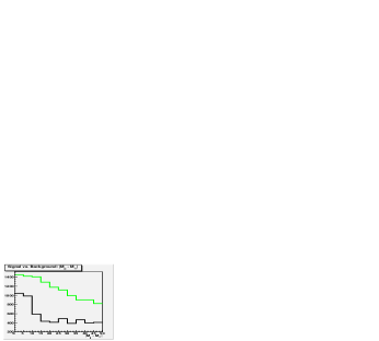
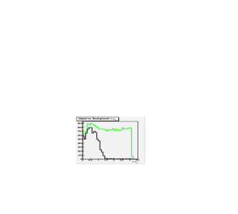
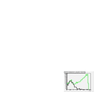
Figure 1: $\Delta M,\Delta\phi_{jj},\ {\rm and}\ \Delta\phi_{\gamma\gamma}$ for the signal (black), and background (gray, green online). The background distribution was constructed with a 50,000 event sample. The signal assumes $m_{h}=120\ {\rm GeV}$, $m_{a}=30\ {\rm GeV}$, and has been scaled up so the distribution shapes shapes can easily be compared. The $\Delta\phi_{jj}$ distribution was created after imposing a $\Delta M<15.0\ {\rm GeV}$ cut.

The signal $\Delta M$ distribution does not change much as $m_{h}$ and $m_{a}$ are varied. From fig. (1) we see that a cut value of $\Delta M\mathrel{\hbox to0.0pt{\raise 2.20013pt\hbox{$<$}\hss}{\lower 2.20013pt\hbox{$\sim$}}}15\ {\rm GeV}$ is most effective. The optimal cut values for $\Delta\phi_{jj}$ and $\Delta\phi_{\gamma\gamma}$ depend on the mass of the pseudoscalar. The lighter the pseudoscalar, the earlier the $\Delta\phi$ distribution peaks, and more background can be excluded. This can be understood from the decay kinematics in the following way. When the Higgs decays into much lighter pseudoscalars, the $a$ will be produced with substantial kinetic energy. Their subsequent decay products (gluons or photons) are predominantly collinear. The higher the velocity, the smaller the average angular separation between the decay products. The most collinear events are removed by our isolation cut, leaving behind a peaked $\Delta\phi$ distribution. In contrast, the background photons (or jets) are emitted primarily back-to-back, where $\Delta\phi_{\gamma\gamma},\Delta\phi_{jj}\approx\pi$. Although a smaller $\Delta\phi$ implies a smaller $\Delta R$, we find the $\Delta\phi$ cuts to be more efficient.

This angular cut is less effective for heavy $a$ which are produced with little kinetic energy. This is offset somewhat by the fact that heavier $m_{a}$ more efficiently pass the $p_{T}>20.0$ cut. Since the kinematics of the signal is least like the background for light $m_{a}$, we will focus on cuts that enhance the significance of that region.

Two variables which often show up in SM $h\rightarrow\gamma\gamma$ searches are $|\cos{\theta^{*}}_{\gamma\gamma}|$ Mrenna:2000qh and photon balance. The first is the scattering angle of the photons calculated in the photon pair rest frame. Cutting on $|\cos{\theta^{*}}|$ has a similar effect to our $\Delta\phi_{\gamma\gamma}$ cut, but it is not as efficient. Photon balance is defined as the ratio of the leading photon $p_{T}$ to the sum of all photon $p_{T}$ unknown:1999fr . We do not find it to be a useful variable for the signal and backgrounds we are considering.

Even with additional angular cuts, the Higgs signal in the majority of parameter space appears only as a slight excess across several bins rather than as a well defined peak. In fact, to get a Higgs peak at any ($m_{h},m_{a}$) point, the branching ratio must be much larger than in our benchmark value. A peak is first visible for $m_{h}\sim 150\ {\rm GeV}$ and $m_{a}\sim 25\ {\rm GeV}$ when $BR(h\rightarrow 2\gamma 2g)\sim 0.04$. Further increasing the branching ratio, the Higgs peak is visible over a wider region of $m_{h},m_{a}$ space - the lower the Higgs mass, the larger the branching ratio needs to be before the peak becomes visible.

Imposing cuts $\Delta\phi_{jj}<1.0,\ \Delta\phi_{\gamma\gamma}<1.3$, and $\Delta M<15\ {\rm GeV}$, the next step is to determine the significance. To determine the significance, we count the number of expected signal and background events in a window $\pm\sqrt{2}\Delta M_{fit}$, where $\Delta M_{fit}$ is the fitted width of the signal. $10\ {\rm GeV}$ bins are used at all times. To make our estimates more realistic, we include the systematic uncertainty of $10\%$ unknown:1999fr ; unknown:2006fr for the overall jet energy scale and jet resolution. The significance including systematic uncertainties is given by unknown:2006fr ; Rainwater:2007cp

$$\frac{S}{\sqrt{B}}\rightarrow\frac{S}{\sqrt{B(1+\Delta^{2}B)}},$$ (9)

where $\Delta$ is the uncertainty. From this significance we calculate the branching ratio necessary for discovery given ${\cal L}=300\ {\rm fb}^{-1}$. The results are shown below in fig. (2).

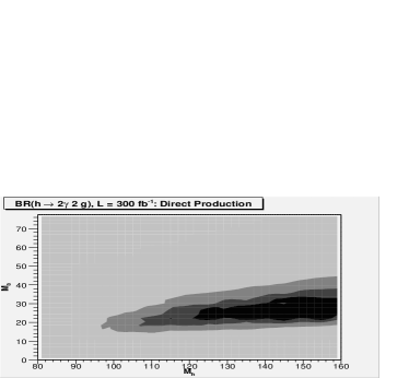
Figure 2: Branching ratio consistent with $S/\sqrt{B}\geq 5.0$ for direct Higgs production with ${\cal L}=300\ {\rm fb}^{-1}$. The contours indicate discovery branching ratios of $\mathrel{\hbox to0.0pt{\raise 2.20013pt\hbox{$<$}\hss}{\lower 2.20013pt\hbox{$\sim$}}}0.06\ {\rm(darkest\ region)},0.1,0.2\ ({\rm lightest})$. Heavy Higgses pass the isolation and $p_{T}$ cuts more easily and are therefore visible at smaller branching ratios. The $m_{a}$ range is restricted above by the $\Delta\phi$ cuts, and below by the isolation cut. We do not consider branching ratios larger than $0.2$.

As expected, a Higgs with the benchmark branching ratio is too small to be detected, even with ${\cal L}=300\ {\rm fb}^{-1}$. Higgses with branching ratio $\sim 0.06$ are visible in a window around $m_{h}\sim 140\ {\rm GeV}$, $m_{a}\sim 20\ {\rm GeV}$, but the size of the detection window doesn’t increase very quickly with increasing branching ratio. Notice that a Higgs lighter than $90\ {\rm GeV}$ require $BR(h\rightarrow 2\gamma 2g)>0.2$. The limited $m_{a}$ extension of the window is a result of the $\Delta\phi$ and isolation cuts. A typical Higgs mass resolution in the discovered region is $\sim\ 10\ {\rm GeV}$.

We used the above procedure in order to get a rough estimates the significance throughout the $m_{h},m_{a}$ parameter space. At any particular $(m_{h},m_{a})$ point, we expect the significance can be improved by further optimizing the cuts and using more sophisticated significance techniques. Another way to improve the significance in this channel is to perform a simultaneous search for the pseudoscalar in $M_{\gamma\gamma}$. Once the pseudoscalar is discovered, the small width of the pseudoscalar will allow us to eliminate a lot of background. Rather than pursue this here, we will move on to a different, cleaner production mode.

IV Associated Production:

The second production mechanism we consider is associated production, $pp\rightarrow W^{\pm}h$. Because we use the hadronic decays of the pseudoscalar, $a\rightarrow jj$, we cannot use the hadronic decays of $W^{\pm}$. The signal is therefore $\ell\kern 2.5pt\raise 0.77496pt\hbox{$/$}\kern-7.5ptE_{T}+\gamma\gamma jj$, $\ell=e,\mu$ which we simulate using PYTHIA. We assume a Standard Model production cross section, and scale our PYTHIA-level cross section to match to match the values in Ref. Djouadi:2005gi . The events are passed through PGS, where leptons are accepted by if they have $p_{T}>5.0\ {\rm GeV}$, if the $p_{T}$ of all tracks within $\Delta R=0.4$ is less than $5.0\ {\rm GeV}$, and if the $E_{T}$ in $3\times 3$ calorimeter segment collar around the lepton is less that $1.1\times$ the $E_{T}$ of the lepton.

The $pp\rightarrow W^{\pm}h$ production cross section at the LHC is smaller than $pp\rightarrow h$ by a factor of $\sim 20$ at $m_{h}\sim 100\ {\rm GeV}$, and it falls off faster with increasing $m_{h}$ Djouadi:2005gi . The smaller cross section, combined with the small branching ratio, means we will have far fewer events at a given luminosity. Because $\sigma(pp\rightarrow Z^{0}h)<\sigma(pp\rightarrow W^{\pm}h)$ and $BR(Z^{0}\rightarrow\ell^{+}\ell^{-})<BR(W\rightarrow\ell\nu)$, we neglect associated $Z^{0}h$ production.

In addition to the cuts for direct production, we impose:

• $1$ lepton with $p_{T}>20\ {\rm GeV},|\eta|<2.5$

• $\Delta R_{\ell-\gamma},\Delta R_{\ell-j}>0.4$

• $\kern 2.5pt\raise 0.77496pt\hbox{$/$}\kern-7.5ptE_{T}>20.0\ {\rm GeV}$

The signal efficiency after the basic cuts varies from $3\%$ to $15\%$ and depends primarily on $m_{a}$. It is highest near $m_{a}\sim 0.5~{}m_{h}$.

IV.1 Background

Fortunately, the background is much smaller than it was for direct production. The lepton and missing energy are useful for reducing the QCD background, and $W+N\ {\rm jets}$ is suppressed by the small jet-$\gamma$ fake rate. The primary background is $W+m\ \gamma+N\ {\rm jets}$, where $m=1,2$ is the number of photons produced with the $W$.

The diphoton background $\gamma\gamma+QCD$, where a jet fakes a lepton, can be sizable if the $\kern 2.5pt\raise 0.77496pt\hbox{$/$}\kern-7.5ptE_{T}$ cut is low. The lepton fake rate is small ${\cal O}(10^{-4})$ :1999fq , but it isn’t enough to completely suppress the large QCD cross sections. With the current cuts we find it constitutes less than $1\%$ of the background. Harder $\kern 2.5pt\raise 0.77496pt\hbox{$/$}\kern-7.5ptE_{T}$ cuts or a cut on the transverse $W$ mass can be imposed to suppress it further.

Another potential background is $\tau^{+}\tau^{-}$ production, where one $\tau$ decays leptonically. These events have a lepton and contain missing energy from the neutrinos in both $\tau$ decays. Photons arise in $\tau$ decay through rare decay modes like $\tau\rightarrow e^{-}\bar{\nu}_{e}\nu_{\tau}\gamma$, through final state radiation, and through hadronic $\tau$ jets faking photons. We estimate that isolation cuts, combined with small branching ratios and the small jet-fake rate, render this background small. We do not include it in the full analysis for simplicity.

The complete set of backgrounds is:

• $W\gamma\gamma+N\ {\rm jets},\ N=0,1,2$

• $W\gamma+{\rm jets}+N\ {\rm jets},\ N=0,1,2$

• $W+N{\rm jets},N=2,3,4$

• ${\rm diphoton+fake\ lepton}$

The $W+{\rm jets}$ and $W+m\ \gamma+N\ {\rm jets}$ backgrounds were simulated using ALPGEN with factorization scale $Q^{2}_{fac}=m^{2}_{W}+p^{2}_{T,W}$. The $K$ factor for $W(\rightarrow\ell\nu)+2\ {\rm jets}$ is $\approx 1$ Oleari:2003tc ; Campbell:2003hd , which we assume for $W(\rightarrow\ell\nu)+{\rm jets}+m\ \gamma$ as well. The diphoton events generated for direct production are used again here with a fake lepton rate $1.25\times 10^{-4}$. As before, all background events were hadronized in PYTHIA and run through PGS.

IV.2 Reconstruction

Combining the two photons with the leading two jets, we form the four body invariant mass $M_{jj\gamma\gamma}$. The signal can be enhanced by imposing $\Delta\phi_{jj}$ and $\Delta\phi_{\gamma\gamma}$ cuts. As in direct production, these cuts are most effective for a light pseudoscalar. It is also helpful to impose the $\Delta M\equiv|m_{jj}-m_{\gamma\gamma}|\leq 20\ {\rm GeV}$ cut. Because there are fewer signal events, we must be careful that the additional cuts to not limit us to $<5$ events (at a given luminosity) necessary for discovery.

After applying angular cuts of $\Delta\phi_{\gamma\gamma}\leq 1.5,\Delta\phi_{jj}\leq 1.3\ {\rm and}\ \Delta M\leq 15\ {\rm GeV}$, we estimate the significance using the same method as in direct production. The Higgs mass resolution is typically $\sim 8-10\ {\rm GeV}$, and we again include a $10\%$ systematic jet energy uncertainty. Using this significance, we calculate the branching ratio required for discovery (significance $>5$) at ${\cal L}=300\ {\rm fb}^{-1}$ as a function of $m_{h}$ and $m_{a}$. It is plotted below in fig. (3).

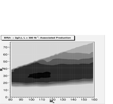
Figure 3: Branching ratio consistent with $S/\sqrt{B}\geq 5.0$ in associated Higgs production with ${\cal L}=300\ {\rm fb}^{-1}$ of luminosity. We require at least $5$ events for discovery. Contours in indicate branching ratios of: $\mathrel{\hbox to0.0pt{\raise 2.20013pt\hbox{$<$}\hss}{\lower 2.20013pt\hbox{$\sim$}}}0.02({\rm darkest\ region}),0.04,0.06,0.1,0.2$ (lightest). The photon reconstruction and cut efficiency increases with $m_{h}$, offsetting the decreasing production cross section.

For $m_{a}$ between $20\ {\rm GeV}$ and $45\ {\rm GeV}$, the branching ratio $BR(h\rightarrow 2\gamma 2g)=0.04$ is sufficient for Higgs discovery for any $m_{h}<160\ {\rm GeV}$ value. The remaining parameter space would be explored with relatively small $\sim{\cal O}(2)$ increases in the branching ratio (or luminosity). Within the narrow range $100\ {\rm GeV}<m_{h}<120\ {\rm GeV}$ and $m_{a}\sim 30\ {\rm GeV}$, a Higgs with even smaller branching ratio would be discovered.

The cut values $\Delta\phi<1.5,\ \Delta\phi_{jj}<1.3$ were chosen to yield high significance for light Higgs masses. The angular cuts are less severe than in direct production, which increases the $m_{a}$ reach of our search. Keeping $m_{a}$ constant and increasing $m_{h}$, we see that the production cross section decreases but the cut efficiency increases. The result is a nearly constant significance. Loosening the $\Delta\phi$ cuts allows us to better probe the $m_{a}>45\ {\rm GeV}$ region, however more sophisticated significance estimates are necessary there because the signal becomes broad.

Simply comparing fig. (3) and the $h\rightarrow 4\gamma$ mode Chang:2006bw using Eq. (5), shows both modes have similar sensitivity for $m_{h}\lessapprox 100\ {\rm GeV}$ while $h\rightarrow 4\gamma$ is more sensitive at larger $m_{h}$. However, this simple comparison somewhat misleading because analysis in Ref. Chang:2006bw was done without a detector simulator. While $h\rightarrow 4\gamma$ will be immune to most complications of a detector simulator, it is sensitive to the photon reconstruction efficiency. We find the photon efficiency using the PGS reconstruction procedure described in section III. to range from $65-80\%$, depending on $m_{h}$ and $m_{a}$. In comparison, Ref. Chang:2006bw used an efficiency of $80\%$. Put on equal footing efficiency-wise, we expect the $h\rightarrow 4\gamma$ and $h\rightarrow 2\gamma 2g$ modes to be comparably sensitive over a wider range of $m_{h},m_{a}$ values and to complement each other well. Because the background in the $h\rightarrow 4\gamma$ mode is so small, it is sensitive to the large-$m_{h}$, large-$m_{a}$ region - exactly the region that is missed in associated production due to the $\Delta\phi$ cuts. Another important aspect that a simple comparison misses is the Higgs mass resolution - $\delta m_{h}\sim 8\ {\rm GeV}$ in $h\rightarrow 2\gamma 2g$ while $\delta m_{h}\sim 1-2\ {\rm GeV}$ in $h\rightarrow 4\gamma$.

V Conclusions:

Electroweak singlets are easy to add to any model of beyond-the-SM physics, and they are even required in some cases. Their presence can cause large deviations from SM Higgs decay patterns. Cascade decays $h\rightarrow aa\rightarrow 4X,X\neq b,\bar{b}$ can naturally dominate in extra-singlet scenarios and will be missed by conventional detection techniques. It is therefore important to investigate where and how the LHC should look to discover this type of Higgs.

The combination of electroweak singlets with two other common new physics features, a ${\cal Z}_{2}$ symmetry and new vector-like fermions, can lead to a Higgs that is particularly difficult to find – Higgses which decay predominantly to gluons and photons and can be as light as $82\ {\rm GeV}$. In this paper we have explored the discovery potential at the LHC for these elusive Higgses using the cascade decay mode $h\rightarrow aa\rightarrow 2\gamma 2g$. We explored the search criteria and the corresponding discovery regions in $m_{h},m_{a}$ space using a benchmark luminosity of ${\cal L}=300\ {\rm fb}^{-1}$ in both direct and associated Higgs production. We generated events using PYTHIA and ALPGEN, and used the detector simulator PGS.

Of the two modes, we find associated production $pp\rightarrow W^{\pm}h\rightarrow\ell\nu+2\gamma 2g$ is sensitive to a wider range of $m_{h},m_{a}$ masses at lower $h\rightarrow 2\gamma 2g$ branching ratio. Imposing cuts on the azimuthal separation of the pseudoscalar decay products, $\Delta\phi_{\gamma\gamma}<1.5,\Delta\phi_{jj}<1.3$ and on the difference between reconstructed pseudoscalar masses $|m_{jj}-m_{\gamma\gamma}|<15\ {\rm GeV}$, we maximize the significance for a light Higgs. Given $300\ {\rm fb}^{-1}$ and $BR(h\rightarrow 2\gamma 2g)\cong 0.04$, we find a $\geq 5\ \sigma$ Higgs signal for $20\ {\rm GeV}<m_{a}<45\ {\rm GeV}$. Isolation cuts prevent us from seeing lighter pseudoscalars, while at larger $m_{a}$ the signal becomes too similar to the background.

Assuming the Higgs always decays to pseudoscalars, associated production is comparable to $h\rightarrow 4\gamma$ for $m_{h}\mathrel{\hbox to0.0pt{\raise 2.20013pt\hbox{$<$}\hss}{\lower 2.20013pt\hbox{$\sim$}}}110\ {\rm GeV}$. Combining both modes will yield greater significance at a given luminosity.

The other mode we considered, direct production $pp\rightarrow h\rightarrow 2\gamma 2g$, has a larger signal but much larger background. Imposing angular cuts eliminates some of the background, but forces us to consider a smaller pseudoscalar mass range. Even with strict angular cuts, only a small slice of parameter space ($m_{h}\mathrel{\hbox to0.0pt{\raise 2.20013pt\hbox{$>$}\hss}{\lower 2.20013pt\hbox{$\sim$}}}120\ {\rm GeV},m_{a}\sim 25\ {\rm GeV}$) would be discovered with the branching ratios of interest.

References

- (1) D. O’Connell, M. J. Ramsey-Musolf, and M. B. Wise, “Minimal extension of the standard model scalar sector,” hep-ph/0611014.
- (2) O. Bahat-Treidel, Y. Grossman, and Y. Rozen, “Hiding the Higgs at the LHC,” hep-ph/0611162.
- (3) V. Barger, P. Langacker, and G. Shaughnessy, “Singlet extensions of the MSSM,” hep-ph/0611112.
- (4) V. Barger, P. Langacker, H.-S. Lee, and G. Shaughnessy, “Higgs sector in extensions of the MSSM,” Phys. Rev. D73 (2006) 115010, hep-ph/0603247.
- (5) V. Barger, P. Langacker, and G. Shaughnessy, “Collider signatures of singlet extended Higgs sectors,” hep-ph/0611239.
- (6) A. Arhrib, K. Cheung, T.-J. Hou, and K.-W. Song, “The light pseudoscalar Higgs boson in NMSSM,” hep-ph/0611211.
- (7) ALEPH Collaboration, S. Schael et. al., “Search for neutral MSSM Higgs bosons at LEP,” Eur. Phys. J. C47 (2006) 547–587, hep-ex/0602042.
- (8) LEP Working Group for Higgs boson searches Collaboration, R. Barate et. al., “Search for the standard model Higgs boson at LEP,” Phys. Lett. B565 (2003) 61–75, hep-ex/0306033.
- (9) “The LEP Electroweak Working Group.” http://lepewwg.web.cern.ch/LEPEWWG/.
- (10) OPAL Collaboration, G. Abbiendi et. al., “Decay-mode independent searches for new scalar bosons with the OPAL detector at LEP,” Eur. Phys. J. C27 (2003) 311–329, hep-ex/0206022.
- (11) J. Erler, “SM Precision Constraints at the LHC/ILC,” hep-ph/0701261.
- (12) S. Chang, P. J. Fox, and N. Weiner, “Naturalness and Higgs decays in the MSSM with a singlet,” JHEP 08 (2006) 068, hep-ph/0511250.
- (13) LEP Higgs Working for Higgs boson searches Collaboration, “Searches for invisible Higgs bosons: Preliminary combined results using LEP data collected at energies up to 209- GeV,” hep-ex/0107032.
- (14) S. Chang, P. J. Fox, and N. Weiner, “Visible cascade Higgs decays to four photons at hadron colliders,” hep-ph/0608310.
- (15) B. A. Dobrescu, G. Landsberg, and K. T. Matchev, “Higgs boson decays to CP-odd scalars at the Tevatron and beyond,” Phys. Rev. D63 (2001) 075003, hep-ph/0005308.
- (16) G. Landsberg and K. T. Matchev, “Discovering a light Higgs boson with light,” Phys. Rev. D62 (2000) 035004, hep-ex/0001007.
- (17) T. Sjostrand, L. Lonnblad, S. Mrenna, and P. Skands, “PYTHIA 6.3: Physics and manual,” hep-ph/0308153.
- (18) CTEQ Collaboration, H. L. Lai et. al., “Global QCD analysis of parton structure of the nucleon: CTEQ5 parton distributions,” Eur. Phys. J. C12 (2000) 375–392, hep-ph/9903282.
- (19) “PGS - Pretty Good Simulator.” http://www.physics.ucdavis.edu/ conway/research/software/pgs/pgs4-general.htm.
- (20) A. Djouadi, “The anatomy of electro-weak symmetry breaking. I: The Higgs boson in the standard model,” hep-ph/0503172.
- (21) M. L. Mangano, M. Moretti, F. Piccinini, R. Pittau, and A. D. Polosa, “ALPGEN, a generator for hard multiparton processes in hadronic collisions,” JHEP 07 (2003) 001, hep-ph/0206293.
- (22) S. Catani, F. Krauss, R. Kuhn, and B. R. Webber, “QCD matrix elements + parton showers,” JHEP 11 (2001) 063, hep-ph/0109231.
- (23) “ATLAS: Detector and physics performance technical design report. Volume 1,”. CERN-LHCC-99-14.
- (24) “ATLAS detector and physics performance. Technical design report. Vol. 2,”. CERN-LHCC-99-15.
- (25) H. Baer, J. Ohnemus, and J. F. Owens, “A NEXT-TO-LEADING LOGARITHM CALCULATION OF DIRECT PHOTON PRODUCTION,” Phys. Rev. D42 (1990) 61–71.
- (26) C. Balazs and C. P. Yuan, “Higgs boson production at hadron colliders with soft gluon effects. I: Backgrounds,” Phys. Rev. D59 (1999) 114007, hep-ph/9810319.
- (27) S. Mrenna and J. D. Wells, “Detecting a light Higgs boson at the Fermilab Tevatron through enhanced decays to photon pairs,” Phys. Rev. D63 (2001) 015006, hep-ph/0001226.
- (28) “CMS TDR Vol. 2,”. report CERN/LHCC/2006-001 (2006).
- (29) D. Rainwater, “Searching for the Higgs boson,” hep-ph/0702124.
- (30) C. Oleari and D. Zeppenfeld, “Next-to-leading order QCD corrections to W and Z production via vector-boson fusion,” Phys. Rev. D69 (2004) 093004, hep-ph/0310156.
- (31) J. Campbell, R. K. Ellis, and D. L. Rainwater, “Next-to-leading order QCD predictions for W + 2jet and Z + 2jet production at the CERN LHC,” Phys. Rev. D68 (2003) 094021, hep-ph/0308195.