Deconfinement transition for nonzero baryon density in the Field Correlator Method.

Abstract

Deconfinement phase transition due to disappearance of confining colorelectric field correlators is described using nonperturbative equation of state. The resulting transition temperature $T_{c}(\mu)$ at any chemical potential $\mu$ is expressed in terms of the change of gluonic condensate $\Delta G_{2}$ and absolute value of Polyakov loop $L_{fund}(T_{c})$, known from lattice and analytic data, and is in good agreement with lattice data for $\Delta G_{2}\approx 0.0035$ GeV⁴. E.g. $T_{c}(0)=0.27;0.19;0.17$ GeV for $n_{f}=0,2,3$ respectively.

1 Introduction

1. Phase transition at nonzero $\mu$ and dynamics of quark gluon plasma (qgp) is now of great interest because of impressive results of heavy ion experiments, see [1] for a recent review and references. The topic calls for a nonperturbative (NP) treatment of QCD degrees of freedom at nonzero $T$ and $\mu$, which is especially important for not very large $T,\mu$. Below we are using the NP approach based on Field Correlator Method (FCM) [2], which was applied to nonzero $T$ in [3, 4].

The main advantage of FCM is a natural explanation and treatment of dynamics of confinement, as well as the deconfinement transition [3, 4], in terms of Color Electric (CE) $D^{E}(x),D^{E}_{1}(x)$ and Color Magnetic (CM) Gaussian (quadratic in $F_{\mu\nu}^{a}$) correlators $D^{H}(x),D_{1}^{H}(x)$.

The correlators $D^{E}(x)$ and $D^{H}(x)$ ensure confinement in the planes $(4,i)$ and $(i,k)$ respectively, $i,k=1,2,3$ so that standard string tension $\sigma^{E}\equiv\sigma=\frac{1}{2}\int D^{E}(x)d^{2}x$, and spatial string tension $\sigma^{H}\equiv\sigma_{s}=\frac{1}{2}\int D^{H}(x)d^{2}x$. Correlators $D^{E}_{1},D^{H}_{1}$ contain perturbative series, and $D_{1}^{E}$ plays an important role in that it contributes to the modulus of the Polyakov line; at $T\geq T_{c}$ one has [5]

$$L_{fund}^{(V)}=|\frac{1}{N_{c}}\langle trP\exp ig\int^{\beta}_{0}A_{4}dz_{4}\rangle|=\exp\left(-\frac{V_{1}(\infty,T)}{2T}\right)$$ (1)

with the static $Q\bar{Q}$ potential

$$V_{1}(r,T)=\int^{\beta}_{0}d\nu(1-\nu T)\int^{r}_{0}\xi d\xi D^{E}_{1}(\sqrt{\xi^{2}+\nu^{2}}).$$ (2)

Deconfinement phase transition in this language is the disappearance of $D^{E}(x)$ (and $\sigma^{E}$) at $T\geq T_{c}$, while $L_{fund}^{(V)}$ and $L_{adj}^{(V)}=(L_{fund}^{(V)})^{9/4}$ are nonzero there.

However the disappearance of $D^{E}(x)=\frac{1}{N_{c}}\langle trE_{i}(x)\Phi(x,y)E_{i}(y)\rangle$ implies vanishing of a part of vacuum energy density,

$$\varepsilon_{vac}=\frac{\beta(\alpha_{s})}{16\alpha_{s}}\langle(F^{a}_{\mu\nu})^{2}\rangle=-\frac{(11-\frac{2}{3}n_{f})}{32}G_{2},~{}~{}D^{E}(0)+D_{1}^{E}(0)+D^{H}(0)+D_{1}^{H}(0)=\frac{\pi^{2}}{9}G_{2}$$ (3)

and $G_{2}$ is the gluon condensate [6]. At $T=0$, $D^{E}=D^{H},D^{E}_{1}=D^{H}_{1}$ and for $T>0$ both $D^{H},D_{1}^{H}$ do not change till $T\approx 2T_{c}$, while $D^{E}$ disappears at $T\geq T_{c}$ [7] in agreement with the deconfinement mechanism suggested in [4].

Particle data [7] and analytic study [8] imply that $D_{1}^{(E,H)}(x)\approx 0.2D^{(E,H)}(x)$, therefore one expects that $\Delta G_{2}=G_{2}(T<T_{c})-G_{2}(T>T_{c})\approx\frac{1}{2}G_{2}(T<T_{c})\approx\frac{1}{2}G_{2}^{st}$, where $G^{st}_{2}\approx 0.012$ GeV⁴ [6] (see [9] for a recent gauge-string duality treatment of $G^{st}_{2}$ yielding $G^{st}_{2}\approx(0.01\pm 0.002)$ GeV⁴).

This $\Delta G_{2}$ taken as the change of free energy (pressure) across the phase boundary will be our basic element in finding the phase transition curve $T_{c}(\mu)$ below.

To this end we introduce in the next section the NP EoS of qgp derived recently in [10], and express $T_{c}(\mu)$ in terms of $\Delta G_{2}$ and $L_{fund}(T_{c})$.

Taking for the latter the lattice or analytic value, one obtains a set of curves $T_{c}(\mu)$ for $n_{f}=0,2,3$ depending on the only parameter $\Delta G_{2}$. These resulting curves and their end points $T_{c}(0),\mu_{c}(0)$ are discussed in conclusion.

2. In the NP approach to the qgp in [10] one introduces in the first approximation the interaction of single quarks and gluons with the vacuum, which is called the Single Line Approximation (SLA), leaving pair and triple, etc… correlations to the next steps. As a result one obtains in SLA the pressure $P_{q}^{SLA}$ of quarks (and antiquarks) and $P_{g}^{SLA}$ of gluons which are expressed through $L_{fund}$, namely [10].

$$p_{q}\equiv{\frac{P^{SLA}_{q}}{T^{4}}}=\frac{4N_{c}n_{f}}{{\pi}^{2}}\sum^{\infty}_{n=1}\frac{(-1)^{n+1}}{n^{4}}L^{n}_{fund}\varphi^{(n)}_{q}cosh\frac{\mu n}{T}$$ (4)

$$p_{gl}\equiv\frac{P_{gl}^{SLA}}{T^{4}}=\frac{2(N^{2}_{c}-1)}{\pi^{2}}\sum^{\infty}_{n=1}\frac{1}{n^{4}}L_{adj}^{n}$$ (5)

with

$$\varphi^{(n)}_{q}(T)=\frac{n^{2}m^{2}_{q}}{2T^{2}}K_{2}\left(\frac{m_{q}n}{T}\right)\approx 1-\frac{1}{4}\left(\frac{nm_{q}}{T}\right)^{2}+...$$ (6)

In (4), (5) it was assumed that $T\mathrel{\mathchoice{\lower 3.6pt\vbox{\halign{$\mathsurround=0pt\displaystyle\hfil#\hfil$\cr<\crcr\sim\crcr}}}{\lower 3.6pt\vbox{\halign{$\mathsurround=0pt\textstyle\hfil#\hfil$\cr<\crcr\sim\crcr}}}{\lower 3.6pt\vbox{\halign{$\mathsurround=0pt\scriptstyle\hfil#\hfil$\cr<\crcr\sim\crcr}}}{\lower 3.6pt\vbox{\halign{$\mathsurround=0pt\scriptscriptstyle\hfil#\hfil$\cr<\crcr\sim\crcr}}}}\frac{1}{\lambda}\cong 1$ GeV, where $\lambda$ is the vacuum correlation length, e.g. $D_{1}^{(E)}(x)\sim e^{-|x|/\lambda}$, hence powers of $L^{n}_{i}$, see [10] for details.

With few percent accuracy one can replace the sum in (5) by the first term, $n=1$, and this form will be used below for $p_{gl}$, while for $p_{q}$ this replacement is not valid for large $\frac{\mu}{T}$, and one can use instead the form equivalent to (4),

$$p_{q}=\frac{n_{f}}{\pi^{2}}\left[\Phi_{\nu}\left(\frac{\mu-\frac{V_{1}}{2}}{T}\right)+\Phi_{\nu}\left(-\frac{\mu+\frac{V_{1}}{2}}{T}\right)\right]$$ (7)

where $\nu=m_{q}/T$ and

$$\Phi_{\nu}(a)=\int^{\infty}_{0}\frac{z^{4}dz}{\sqrt{z^{2}+\nu^{2}}}\frac{1}{(e^{\sqrt{z^{2}+\nu^{2}}-a}+1)}.$$ (8)

Eqs. (7), (5) define $p_{q},p_{gl}$ for all $T,\mu$ and $m_{q}$, which is the current (pole) quark mass at the scale of the order of $T$.

Using (4-(8) we can define the pressure $P_{I}$ in the confined phase, and $P_{II}$ in the deconfined phase, taking into account that vacuum energy density in two phases $\varepsilon_{vac}$ and $\varepsilon_{vac}^{dec}$ respectively contributes to the free energy, and hence $|\varepsilon_{vac}|,|\varepsilon_{vac}^{dec}|$ to the pressure. One has

$$P_{I}=|\varepsilon_{vac}|+P_{hadron},~{}~{}P_{II}=|\varepsilon_{vac}^{dec}|+(p_{gl}+p_{q})T^{4}.$$ (9)

Here $P_{hadron}$ is the pressure of the hadron gas at $T\leq T_{c}$. From $P_{I}(T_{c})=P_{II}(T_{c})$ one obtains $T_{c}$, neglecting $P_{hadron}$ in the first approximation

$$T_{c}(\mu)=\left(\frac{(11-\frac{2}{3}n_{f})\Delta G_{2}}{32(p_{gl}+p_{q})}\right)^{1/4}.$$ (10)

In (10) enter only two parameters; $\Delta G_{2}$ and $L_{fund}(T_{c})=\exp\left(-\frac{\kappa}{T_{c}}\right)$, $\kappa\equiv\frac{1}{2}{V_{1}(\infty,T_{c})}\cong\frac{1}{2}F^{1}_{Q\bar{Q}}(\infty,T_{c})$.

The latter can be found in 3 different ways: 1) from the direct lattice measurements [11] of $P^{1}_{Q\bar{Q}}\approx 0.5$ GeV; 2) from analytic calculation of $D_{1}^{E}$ in [8], which yields $V_{1}(\infty,T<T_{c})\approx\frac{6\alpha_{s}(M_{0})\sigma}{M_{0}}\approx 0.5$ GeV with $M_{0}\cong(0.8-1)$ GeV lowest gluelump mass [12]; 3) from lattice calculations of $D_{1}^{E}$ at $T>T_{c}$, [7, 13], which according to (2) yields $V_{1}(\infty,T_{c})\approx 0.4\div 0.6$ GeV. Therefore one can fix $V_{1}(\infty,T_{c})=0.50(5)$ GeV ($\kappa=0.25$ GeV) and this value is independent of $n_{f}$ [11]. As a result $T_{c}(\mu)$ is a function of only $\Delta G_{2}$ and for each value of $\Delta G_{2}$ one finds a set of curves for $n_{f}=2,3,...$ We choose $\Delta G_{2}\approx\frac{1}{2}G_{2}^{st}$ and in Fig.1 the curves computed numerically from (10) for $n_{f}=2,3$ are shown for $\Delta G_{2}\approx 0.00341$ GeV⁴ and zero quark pole masses.

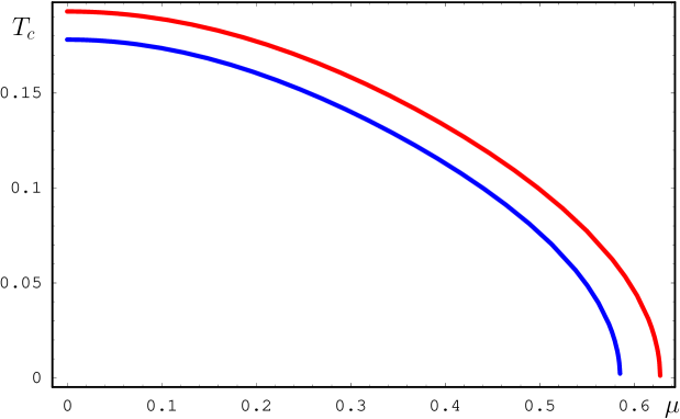
Figure 1: The phase transition curve $T_{c}(\mu)$ from Eq.(10) (in GeV) as function of quark chemical potential $\mu$ (in GeV) for $n_{f}=2$ (upper curve) and $n_{f}=3$ (lower curve) and $\Delta G_{2}=0.0034$ GeV⁴.

.

The end points $T_{c}(0)$ and $\mu_{c}(0)$ can be found analytically e.g. for $T_{c}(\mu)$ with $\sim 5\%$ accuracy one has (expanding (10) in $\frac{p_{gl}}{p_{q}})$

$$T_{c}(\mu)=T_{c}(0)\left(1-C\frac{9\mu^{2}}{T^{2}_{c}(0)}\right),~{}~{}C=0.0110(3),$$ (11)

with

$$T_{c}(0)\approx\frac{1}{2}T^{(0)}\left(1+\sqrt{1+\frac{\kappa}{T^{(0)}}}\right),~{}~{}T^{(0)}=\left(\frac{(11-\frac{2}{3}n_{f})\pi^{2}\Delta G_{2}}{384n_{f}}\right)^{1/4}.$$ (12)

For $\Delta G_{2}=0.00341$ GeV⁴ one obtains $T_{c}(0)=(0.27;0.19;0.17)$ GeV for $n_{f}=0,2,3$ respectively, which agrees well with numerous lattice data, see [14] for reviews. The value of $C=0.011$ is inside the scattered set of lattice values [14].

Another end point, $\mu_{c}(0)$ can be found from the asymptotics of (8), $\Phi_{0}(a\to\infty)=\frac{a^{4}}{4}+\frac{\pi^{2}}{2}a^{2}+...,$ which yields (for $m_{q}=0)$ $\mu_{c}(0)=\kappa+(48)^{1/4}T^{(0)}$ and for the same $\Delta G_{2}$ as above one gets $\mu_{c}(0)=(0.63;0.58)$ GeV for $n_{f}=2,3$ One can check, that the derivative in $T$, $\frac{d\mu_{c}(T)}{dT}$ vanishes at $T=0$.

3. The phase curve $T_{c}(\mu)$ in Fig.1 is in reasonable agreement with lattice data at least for $\mu\mathrel{\mathchoice{\lower 3.6pt\vbox{\halign{$\mathsurround=0pt\displaystyle\hfil#\hfil$\cr<\crcr\sim\crcr}}}{\lower 3.6pt\vbox{\halign{$\mathsurround=0pt\textstyle\hfil#\hfil$\cr<\crcr\sim\crcr}}}{\lower 3.6pt\vbox{\halign{$\mathsurround=0pt\scriptstyle\hfil#\hfil$\cr<\crcr\sim\crcr}}}{\lower 3.6pt\vbox{\halign{$\mathsurround=0pt\scriptscriptstyle\hfil#\hfil$\cr<\crcr\sim\crcr}}}}0.25$ GeV, see [15] for review and references. Two important points are to be discussed here: 1) order of transition and possible critical point 2) approximations and assumptions of the present work.

1). The vacuum transition of our approach is evidently of the first order at least in the leading (SLA) approximation used for (10), and does not contain any critical points. This is in agreement with lattice $n_{f}=0$ data, but the lattice results for $n_{f}=2,3$ depend on masses, discretization and are not fully conclusive. The softening of transition for $n_{f}>0$ in our approach is explained by the increasing role of $P_{hadron}(T)$ for $n_{f}>0$ near $T_{c}$, which suppresses the specific heat and makes the curve $P(T)$ more smooth. The chiral transition in our approach is caused by the deconfinement, since both $\langle\bar{q}q\rangle$ and $f_{\pi}$ are expressed via $D^{E}(x)$ [16] and vanish together with it, in agreement with lattice data, see e.g. [14]. The Polyakov loop is a good (approximate) order parameter for $n_{f}=0(n_{f}>0)$ since at $T<T_{c}$ it is expressed via $D^{E}(x)$ and vanishes (strongly decreases) (see Eq. (6) of [5]).

2) In our derivation of (10)-(12) it was assumed a) that the only important part of qgp dynamics is the interaction with the NP vacuum –SLA; b) it is assumed that vacuum fields do not depend on $T,\mu$ in the phase diagram, except at the phase boundary where the shift $\Delta G_{2}$ occurs; in particular neither $\Delta G_{2}$ nor $L_{fund}(T_{c})$ depend on $\mu$. The latter point is partly supported by lattice data [17]. In general this picture of rigid vacuum is based on the notion of the dilaton scale $m_{d}$ of vacuum fields, which can be associated with the $0^{++}$ glueball mass around 1.5 GeV and therefore for all external parameters (like $\mu$ or $T$) much less than $m_{d}$ vacuum fields are fixed.

Another argument in favor of rigid vacuum is that all dependence on $\mu$ and $n_{f}$ does not appear in the lowest order of $1/N_{c}$ expansion, since it comes from the quark loops. (Note that nevertheless $T_{c}(0)$ differs strongly for $n_{f}=0$ and $n_{f}=2,3$; even through $\Delta G_{2}$ was kept fixed, and this successful prediction of $T_{c}(0)=0.27$ GeV and 0.19 GeV respectively can be considered as another support of our picture). Several things were not taken into account. Quark masses are included trivially via Eqs.(6,7) and this can be checked $vs$ lattice data. Phase transition near $\mu_{c}(0)$ can be complicated due to strong $qq$ and $qqq$ interaction, which is not taken into account above and will be discussed elsewhere (see also [10]). therefore the possibility of color superconductivity is not commented here.

The authors are grateful for useful discussions to members of ITEP seminar. The financial support of RFBR grants 06-02-17012, grant for scientific schools NSh-843.2006.2 and the State Contract 02.445.11.7424 is gratefully acknowledged. This work was done with financial support of the Federal Agency of Atomic Energy.

References

- [1] J.-P.Blaizot,Plenary talk at QM 2006, Shanghai, hep-ph/0703150.
- [2] H.G.Dosch, Phys. Lett B190, 177 (1987); H.G.Dosch, Yu.A.Simonov, Phys. Lett. B 205, 339 (1988); Yu.A.Simonov, Nucl. Phys. B 307, 512 (1988); A.Di Giacomo, H.G.Dosch, V.I.Shevchenko, Yu.A.Simonov, Phys. Rep. 372, 319 (2002).
- [3] Yu.A.Simonov, Phys. At. Nucl. 58, 309 (1995);hep-ph/9311216; Yu.A.Simonov, In ”Varenna 1995, Selected topics in nonperturbative QCD”, p.319; hep-ph/9509404; E.L.Gubankova and Yu.A.Simonov, Phys. Lett. 360, 93 (1995).
- [4] Yu.A.Simonov, JETP Lett. 55, 627 (1992); Yu.A.Simonov, JETP Lett. 54, 249 (1991).
- [5] Yu.A.Simonov, Phys. Lett. B 619, 293 (2005).
- [6] M.Shifman, A.Vainshtein, V.Zakharov, Nucl. Phys. B 147, 385, 448 (1979).
-
[7]
A.Di Giacomo and H.Panagopoulos, Phys. Lett. B 285, 133 (1992);
M.D’Elia, A.Di Giacomo and E.Meggiolaro, Phys. Lett. B 408, 315 (1997);
A.Di Giacomo, E.Meggiolaro and H.Panagopoulos, Nucl. Phys. B 483, 371 (1997);
G.S.Bali, N.Brambilla, A.Vairo, Phys. Lett. B 421, 265 (1998). - [8] Yu.A.Simonov, Phys. At. Nucl. 69, 528 (2006) hep-ph/0501182.
- [9] O.Andreev, V.I.Zakharov, hep-ph/0703010.
- [10] Yu.A.Simonov, hep-ph/0702266.
- [11] O.Kaczmarek, F.Zantov, hep-lat/0506019.
- [12] Yu.A.Simonov, Nucl. Phys. B592, 350 (2001).
- [13] A.Di Giacomo, E. Meggiolaro, Yu.A.Simonov, A.I.Veselov, hep-ph/0512125, Phys.At. Nucl. (in press).
- [14] C.Schmidt, hep-lat/0701019; C.Bernard et al., hep-lat/0611031; R.Gavai, hep-ph/0607050; U.M.Heller, hep-lat/0610114; F.Karsch, hep-lat/0601013, hep-lat/0608003.
- [15] C.R.Allton, S.Ejiri, S.J.Hands, et al., hep-lat/0504011; Z.Fodor, S.D.Katz, C.Schmidt, hep-lat/0701022; M.P.Lombardo, hep-lat/0612017.
- [16] Yu.A.Simonov, Phys. Atom. Nucl., 60, 2069 (1997), hep-ph/9704301; Phys. Rev. D65, 094018 (2002); Yu.A.Simonov, Phys. Atom. Nucl. 67, 1027 (2004), hep-ph/0305281.
- [17] M.Döring, S.Ejiri, O.Kaczmarek, F.Karsch, E.Laermann, hep-lat/0509001.