Phenomenological analysis of two-photon exchange effects
in proton form factor measurements

Abstract

We perform a model-independent phenomenological analysis of experimental data on proton form factor ratio. We find that only one of the two-photon exchange amplitudes, which we call $\delta{\cal G}_{M}$, is responsible for the discrepancy between Rosenbluth and polarization methods. The linearity of Rosenbluth plots implies that $\delta{\cal G}_{M}$ is approximately linear function of $\varepsilon$. The slope of $\delta{\cal G}_{M}$ is extracted from experimental data and is shown to be consistent with theoretical calculations.

At present, proton form factors (FFs) are measured with two techniques: Rosenbluth or longitudinal-transverse (LT) separation and polarization transfer (PT). The latter technique gives only FF ratio $G_{E}/G_{M}$. When the experiments by the PT method were extended to $Q^{2}\geq 2{\rm\ GeV}^{2}$, the results have shown clear deviation from those of Rosenbluth method HowWell . Two-photon exchange (TPE) effects are generally believed to be the cause for this discrepancy. They were studied both phenomenologically GV ; Tvaskis ; C and theoretically Blunden ; BMT ; BMTdelta ; we ; GPD . The theoretical calculation of TPE effects is nontrivial and technically difficult. On the other hand, assuming that the discrepancy is entirely due to TPE, one can extract some information on TPE directly from experiment. The values of TPE amplitudes, obtained in such a manner in Ref.GV , are in serious disagreement with the theoretical estimates. In the present paper we extract the TPE amplitudes from experiment more correctly and demonstrate that they agree with theoretical calculations.

The following notation is used: particle momenta are defined by ${\rm e}(k)+{\rm p}(p)\to{\rm e}(k^{\prime})+{\rm p}(p^{\prime})$; $K=(k+k^{\prime})/2$, $P=(p+p^{\prime})/2$, $\nu=4PK$, transferred momentum is $q=p^{\prime}-p$, $Q^{2}=-q^{2}$, the proton mass is $M$; the virtual photon polarization parameter is $\varepsilon=\frac{\nu^{2}-Q^{2}(4M^{2}+Q^{2})}{\nu^{2}+Q^{2}(4M^{2}+Q^{2})}$.

In general case the amplitude of the elastic electron-proton scattering can be written as GV

$${\cal M}=\frac{4\pi\alpha}{Q^{2}}\bar{u}^{\prime}\gamma_{\mu}u\cdot\bar{U}^{\prime}\left(\tilde{F}_{1}\gamma^{\mu}-\tilde{F}_{2}[\gamma^{\mu},\gamma^{\nu}]\frac{q_{\nu}}{4M}+\tilde{F}_{3}K_{\nu}\gamma^{\nu}\frac{P^{\mu}}{M^{2}}\right)U$$ (1)

(the terms proportional to the electron mass are neglected). Invariant amplitudes (also called generalized FFs) $\tilde{F}_{i}$ are scalar functions of two kinematic variables, say, $Q^{2}$ and $\varepsilon$. For our purpose it is convenient to introduce linear combinations

$${\cal G}_{E}=\tilde{F}_{1}-\tau\tilde{F}_{2}+\frac{\nu}{4M^{2}}\tilde{F}_{3},\ \ \ {\cal G}_{M}=\tilde{F}_{1}+\tilde{F}_{2}+\varepsilon\frac{\nu}{4M^{2}}\tilde{F}_{3},\ \ \$$ (2)

where $\tau=\frac{Q^{2}}{4M^{2}}$. In general, the amplitudes are complex, but their imaginary parts give negligible contribution to the observables considered here. Thus later on, speaking of the amplitudes, we understand their real parts.

With amplitudes (2), the reduced cross-section for unpolarized particles can be written like the Rosenbluth formula

$$\frac{(1-\varepsilon)}{32\alpha^{2}}Q^{2}\left(\frac{\nu+Q^{2}}{\nu-Q^{2}}\right)^{2}\frac{d\sigma}{d\Omega_{lab}}\equiv\sigma_{R}=\varepsilon{\cal G}_{E}^{2}+\tau{\cal G}_{M}^{2}+O(\alpha^{2}).$$ (3)

The amplitudes can be decomposed as

$${\cal G}_{E}(Q^{2},\varepsilon)=G_{E}(Q^{2})+\delta G_{E}^{(T)}(Q^{2},\varepsilon)+\delta{\cal G}_{E}(Q^{2},\varepsilon)+O(\alpha^{2})$$ (4)

and similarly for ${\cal G}_{M}$; $G_{E}$ and $G_{M}$ are proton electric and magnetic FFs and $\delta G_{E,M}^{(T)}+\delta{\cal G}_{E,M}$ are TPE corrections of order $\alpha$. Here $\delta G_{E,M}^{(T)}$ denotes the part of the correction, calculated by Tsai Tsai . All infrared divergence is contained in it. The reduced cross-section then takes the form

$$\sigma_{R}=\varepsilon G_{E}^{2}+\tau G_{M}^{2}+2\varepsilon G_{E}\delta{\cal G}_{E}+2\tau G_{M}\delta{\cal G}_{M}+2\varepsilon G_{E}\delta G_{E}^{(T)}+2\tau G_{M}\delta G_{M}^{(T)}+O(\alpha^{2}).$$ (5)

The terms containing $\delta G_{E,M}^{(T)}$ are always subtracted from the cross-section by experimenters as a part of radiative corrections, so published cross-sections are, dropping terms of order $\alpha^{2}$,

$$\sigma_{R}=\varepsilon G_{E}^{2}+\tau G_{M}^{2}+2\varepsilon G_{E}\delta{\cal G}_{E}+2\tau G_{M}\delta{\cal G}_{M}.$$ (6)

These cross-sections are used as an input for the Rosenbluth separation.

Now we will analyze Eq.(6) in the case of $\tau\gtrsim 1$.

Since the TPE amplitudes are proportional to $\alpha\approx\frac{1}{137}$, it is natural to believe that their magnitude is about 1%. The key point is that $G_{M}$ is enhanced with respect to $G_{E}$ by about a factor of $\mu\approx 3$ (proton magnetic moment), and even more according to PT data, so we have

$$\tau G_{M}^{2}\gg\varepsilon G_{E}^{2}\gg 2\varepsilon G_{E}\delta{\cal G}_{E},\ \ \tau G_{M}^{2}\gg 2\tau G_{M}\delta{\cal G}_{M}\gg 2\varepsilon G_{E}\delta{\cal G}_{E}.$$ (7)

Therefore the term $2\varepsilon G_{E}\delta{\cal G}_{E}$ is much smaller than three other terms and can be safely neglected. Instead, the term $2\tau G_{M}\delta{\cal G}_{M}$ can be comparable with $\varepsilon G_{E}^{2}$ and thus strongly affect the results of Rosenbluth separation. We take for granted that Rosenbluth plots are linear (recent analyses Tvaskis ; C confirm this), i.e. $\sigma_{R}$ is linear function of $\varepsilon$. This necessarily leads to the conclusion, that $\delta{\cal G}_{M}$ is also approximately linear; we write it as

$$\delta{\cal G}_{M}(Q^{2},\varepsilon)=[a(Q^{2})+\varepsilon b(Q^{2})]G_{M}(Q^{2}),$$ (8)

where $a$ and $b$ are of order $\alpha$. The coefficient $a$ yields only a small contribution to the large $\varepsilon$-independent term in $\sigma_{R}$ and does not change $\varepsilon$-dependent term, thus we also may neglect it. After that

$$\sigma_{R}=\tau G_{M}^{2}+\varepsilon(G_{E}^{2}+2\tau b\,G_{M}^{2})$$ (9)

and the FF ratio squared obtained by the Rosenbluth method is actually

$$\biggl{.}\left(\frac{G_{E}}{G_{M}}\right)^{2}\biggr{|}_{LT}\equiv R_{LT}^{2}=\frac{G_{E}^{2}}{G_{M}^{2}}+2\tau b.$$ (10)

The FF ratio obtained in the PT experiments (with the inclusion of TPE) can be written as

$$\left.\frac{G_{E}}{G_{M}}\right|_{PT}\equiv R_{PT}=\frac{{\cal G}_{E}}{{\cal G}_{M}}\left(1-\frac{\varepsilon(1-\varepsilon)}{1+\varepsilon}Y_{2\gamma}\right)+O(\alpha^{2}),$$ (11)

where $Y_{2\gamma}=\frac{\nu}{4M^{2}}\frac{\tilde{F}_{3}}{G_{M}}$. The quantity $\frac{\varepsilon(1-\varepsilon)}{1+\varepsilon}$ never exceeds 0.17 and $Y_{2\gamma}$ should be about 1%, thus the bracket is very close to 1. Also, since the corrections $\delta{\cal G}_{E}$ and $\delta{\cal G}_{M}$ amount to about 1%, the ratio ${\cal G}_{E}/{\cal G}_{M}$ is close to $G_{E}/G_{M}$ and anyway matches it within the experimental errors, which are typically about 5%. Therefore we may say that PT experiments yield true FF ratio

$$R_{PT}=\frac{G_{E}}{G_{M}}.$$ (12)

Substituting (12) into (10), we obtain the TPE correction slope

$$b=\frac{1}{2\tau}(R_{LT}^{2}-R_{PT}^{2}).$$ (13)

We fitted $R_{PT}^{2}$ from Ref.PT and $R_{LT}^{2}$ from Ref.LT with polynomials in $Q^{2}$ of the third order to minimize the $\chi^{2}$ function

$$\chi^{2}=\sum_{i}\left(\frac{R_{i}^{2}-P(Q^{2}_{i})}{2R_{i}\Delta R_{i}}\right)^{2},$$ (14)

where $\Delta R_{i}$ are experimental errors. We have obtained, for Rosenbluth data

$$P_{LT}(Q^{2})=\mu^{-2}(1.0736-0.1864Q^{2}+0.0358Q^{4}+0.0007Q^{6})$$ (15)

with $\chi^{2}=24.2$ for 28 d.o.f. and for PT data

$$P_{PT}(Q^{2})=\mu^{-2}(1.1184-0.3256Q^{2}+0.0323Q^{4}-0.0014Q^{6})$$ (16)

with $\chi^{2}=6.6$ for 15 d.o.f. (everywhere $Q$ is in units of GeV and $\mu=2.793$). The results are shown in Fig.1.

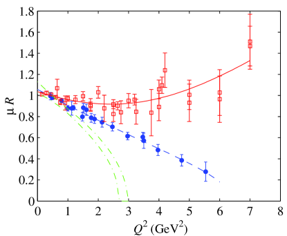
Figure 1: (Color online) Experimental data and fits to FF ratio obtained by Rosenbluth method ($\mu R_{LT}$, solid curve and squares) and by PT method ($\mu R_{PT}$, dashed curve and circles) and prediction for Rosenbluth method with positrons (dash-dotted curves, $1\sigma$ range).

From this we derive the coefficient $b$:

$$b=-0.0101/Q^{2}+0.0314+0.0008Q^{2}+0.0005Q^{4}.$$ (17)

The dependence of $b$ vs. $Q^{2}$ is displayed in Fig.2. The coefficient $a$ cannot be derived from the experimental data.

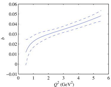
Figure 2: (Color online) Extracted TPE correction slope $b(Q^{2})$. The dashed curves indicate estimated errors.

We see that $b$ varies from 0.01 to 0.05; if the unknown coefficient $a$ is negative and equals about $-b/2$ then the relative size of TPE correction $\delta{\cal G}_{M}/G_{M}=a+\varepsilon b$ will never exceed 0.025, in consistency with the assumptions made at the very beginning.

From the theoretical point of view, the TPE corrections can be split into elastic and inelastic parts. The elastic part was first calculated in Ref. Blunden using simple monopole parameterization of FFs and then in a model-independent way in Refs. BMT ; we . The inelastic part is at present modeled by resonances BMTdelta or by parton models GPD . In Fig.3 we plot the elastic part of $\delta{\cal G}_{M}$, calculated as described in Ref.we and straight line according to Eq.(8) with $b$ given above and $a$ chosen arbitrarily. A qualitative agreement is seen at all values of $Q^{2}$. The gap between the curve and the line is small and should be possibly attributed to inelastic contribution. This results differ from those of Ref.GV , where authors, in fact, made three arbitrary assumptions about the TPE amplitudes (namely, in the notation of Ref.GV , that $Y_{2\gamma}$, $|\tilde{G}_{E}|$, and $|\tilde{G}_{M}|$ are all independent of $\varepsilon$), and obtained the quantity $Y_{2\gamma}$ approximately 5 times larger than theoretical estimates BMT .

Figure 3: (Color online) Comparison of extracted (dashed lines) and calculated (solid curves) values of TPE amplitude $\delta{\cal G}_{M}/G_{M}$.

If the positrons are used instead of electrons, the TPE corrections change their sign. Thus we have for the Rosenbluth FF ratio squared, measured in positron-proton scattering

$$\tilde{R}_{LT}^{2}=\frac{G_{E}^{2}}{G_{M}^{2}}-2\tau b$$ (18)

(Fig.1, where dash-dotted lines indicate estimated $1\sigma$ bounds for $\mu\tilde{R}_{LT}$). The values of $\tilde{R}_{LT}^{2}$ strikingly differ from $R_{LT}^{2}$ and become even negative for $Q^{2}>3{\rm\ GeV}^{2}$. Therefore the Rosenbluth measurements with positron beam at $Q^{2}\gtrsim 2{\rm\ GeV}^{2}$ would be an interesting test for TPE effects, and, on the other hand, a new way to measure true FF ratio, since the TPE corrections fully cancel in the average of $R_{LT}^{2}$ and $\tilde{R}_{LT}^{2}$. Precision study of positron-proton cross-section is already proposed, for $Q^{2}\lesssim 1.6{\rm\ GeV}^{2}$ VEPP and for $0.5<Q^{2}<3{\rm\ GeV}^{2}$ E04 .

References

(1) J. Arrington, Phys. Rev. C 68, 034325 (2003).
(2) P.A.M. Guichon, M. Vanderhaeghen, Phys. Rev. Lett. 91, 142303 (2003).
(3) V. Tvaskis et al., Phys. Rev. C 73, 025206 (2006).
(5) P.G. Blunden, W. Melnitchouk, J.A. Tjon, Phys. Rev. Lett 91, 142304 (2003).
(6) P.G. Blunden, W. Melnitchouk, J.A. Tjon, Phys. Rev. C 72, 034612 (2005).
(7) S. Kondratyuk, P.G. Blunden, W. Melnitchouk, J.A. Tjon, Phys. Rev. Lett. 95, 172503 (2005).
(8) D. Borisyuk, A. Kobushkin, Phys. Rev. C 74, 065203 (2006).
(9) Y.C. Chen et al., Phys. Rev. Lett. 93, 122301 (2004).
(10) Y.S. Tsai, Phys. Rev. 122, 1898 (1961).
(11) O. Gayou et al., Phys. Rev. Lett. 88, 092301 (2002); V. Punjabi et al., Phys. Rev. C 71, 055202 (2005); G. MacLachlan et al., Nucl. Phys. A764, 261 (2006); M.K. Jones et al., Phys. Rev. C 74, 035201 (2006).
(12) I.A. Qattan et al., Phys. Rev. Lett. 94, 142301 (2005); M.E. Christy et al., Phys. Rev. C 70, 015206 (2004); L. Andivahis et al., Phys. Rev. D 50, 5491 (1994); R.C. Walker et al., Phys. Rev. D 49, 5671 (1994).
(13) J. Arrington et al., nucl-ex/0408020.
(14) Jefferson Lab experiment E04-116, W.Brooks et al. spokespersons.