Anthropic tuning of the weak scale and of $m_{u}/m_{d}$ in two-Higgs-doublet models

Abstract

It is shown that in a model in which up-type and down-type fermions acquire mass from different Higgs doublets, the anthropic tuning of the Higgs mass parameters can explain the fact that the observed masses of the $d$ and $u$ quarks are nearly the same with $d$ slightly heavier. If Yukawa couplings are assumed not to “scan” (vary among domains), this would also help explain why $t$ is much heavier than $b$. It is also pointed out that the existence of dark matter invalidates some earlier anthropic arguments against the viability of domains where the Standard Model Higgs has positive $\mu^{2}$, but makes other even stronger arguments possible.

1 Introduction

The mass parameter of the Higgs field in the Standard Model ($\mu^{2}$) gives the appearance of being “anthropically tuned” [1]. That is, if one imagines the other parameters of the Standard Model to be fixed, and considers what the universe would look like for different values of $\mu^{2}$, one finds that organic life may only be possible if $\mu^{2}$ is negative and has a magnitude very close to the value actually observed. From the physics point of view this might be just a coincidence, though a remarkable one. On the other hand, as pointed out by Ref. [1], it might have a physical explanation in the context of “many-domain”, “multiverse”, “landscape” scenarios. (These are equivalent names for the same idea. For recent reviews see [2].) An explanation of that sort would account for the closeness of the strong-interaction and weak-interaction scales ($M_{strong}/M_{P\ell}\sim 10^{-19}$ and $M_{weak}/M_{P\ell}\sim 10^{-17}$), something not yet explained by any other scenario. (The nearness of the weak-scale to the strong scale results in the lightest quarks having masses small compared to $\Lambda_{QCD}$, which in turn leads to the existence of nonperturbative bound states of quarks, pseudogoldstone pions, and the the richness of hadronic and nuclear physics, and consequently of chemistry.)

In this paper we extend the analysis of [1] to a slightly more general Higgs structure and show that a possible anthropic explanation of the fact that $m_{u}/m_{d}\sim 1$ emerges. We also reconsider the crucial case of positive $\mu^{2}$, and point out that one of the anthropic arguments proposed in [1] to exclude most of the $\mu^{2}>0$ region is invalidated by the existence of dark energy (which had not yet been discovered when [1] was written). However, we show that the existence of dark energy makes possible a very different set of arguments that reach even stronger conclusions.

The papers of Ref. 1 assumed that the only parameter of the Standard Model that varies among domains and is anthropically tuned is $\mu^{2}$. Several facts suggest the possibility that the observed value of $\mu^{2}$ may be acounted for in a different way than the values of the other parameters of the Standard Model. First, $\mu^{2}$ is the only dimensionful parameter of the Standard Model Lagrangian. Second, it is the most highly tuned of the Standard Model parameters, being $10^{-34}$ of its “natural” value. (The next most tuned parameter is $\overline{\theta}$, which is less than $10^{-9}$ of its natural value.) Third, the smallness of $\mu^{2}$ is so far the most intractable of the naturalness problems of the Standard Model. Various plausible mechanisms of a more conventional sort have been proposed for explaining the smallness of other Standard Model parameters. (For example, the smallness of $\overline{\theta}$ can be explained by the Peccei-Quinn mechanism [3] or by spontaneously broken CP or P [4]; and various symmetry schemes have been proposed to explain the smallness of the Yukawa couplings of the light quarks and leptons). By contrast, attempts to explain the smallness of the weak scale by technicolor or similar ideas are plagued by a variety of well-known difficulties. And low energy supersymmetry does not by itself explain the magnitude of the weak scale, though it protects it from radiative correction.

Since the focus of Ref. 1 was on the mass parameter of the Higgs field, the question naturally arises how things would be different if there were two or more Higgs doublets. Two Higgs doublets appear in a wide variety of theoretical contexts: in theories with supersymmetry; in Peccei-Quinn models; and in many grand unified models (such as $SO(10)$, if the ${\bf 10}$ of Higgs fields is assumed to be complex). The simplest possibility, which is typical of the above-mentioned scenarios, and which avoids problems of Higgs-mediated flavor-changing processes, is that one doublet ($H_{u}$) couples to the up-type quarks, while the other doublet ($H_{d}$) couples to the down-type quarks and charged leptons [5]. It is this situation we will analyze in this paper. Thus, at high scales we have

$$\begin{array}[]{ccl}{\cal L}_{Yuk}&=&(Y_{u}\overline{u}u+Y_{c}\overline{c}c+Y_{t}\overline{t}t)H_{u}\\ &&\\ &+&(Y_{d}\overline{d}d+Y_{s}\overline{s}s+Y_{b}\overline{b}b)H_{d}+(Y_{e}\overline{e}e+Y_{\mu}\overline{\mu}\mu+Y_{\tau}\overline{\tau}\tau)H_{d}.\end{array}$$ (1)

With two Higgs doublets, there are several dimensionful Higgs-mass parameters that may vary among domains, with the consequence that $\langle H_{u}\rangle=v_{u}$ and $\langle H_{d}\rangle=v_{d}$ may vary independently. This means that there is the possibility of explaining not only the magnitude of the weak scale, but also the relative magnitudes of the masses of the up-type and down-type quarks. In particular, we shall see that an explanation of the size of $m_{u}/m_{d}$ and thus a partial explanation of $m_{t}/m_{b}$ emerges. Much of our analysis would apply equally to models with or without low-energy supersymmetry, and would apply in fact to any model where in effect both $v_{u}$ and $v_{d}$ vary among domains. Thus, the “anthropic” considerations given in this paper are not proposed as an alternative to low-energy supersymmetry. Indeed, they may shed light eventually on supersymmetry-breaking and the $\mu$ problem. However, in this paper we will consider for purposes of concreteness a non-supersymmetric two-Higgs-doublet model.

In such a model, the parameter $\mu^{2}$ is replaced by a two-by-two Hermitian mass matrix $M^{2}_{ij}$, $i,j=u,d$, with four real parameters. To make the weak-scale small, still only one tuning is required, namely of the determinant of $M^{2}_{ij}$, since only one Higgs doublet needs to remain light to break $SU(2)_{L}\times U(1)_{Y}$. The other doublet has no reason to be light, and in fact would be expected to be of superlarge mass. The doublet that is light (whose mass-squared we shall call $\mu^{2}$) is a linear combination of $H_{u}$ and $H_{d}$: $H_{<}=\sin\beta H_{u}+\cos\beta\tilde{H}_{d}$, where $\tilde{H}_{d}\equiv i\tau_{2}H_{d}^{*}$. The mixing angle $\beta$ enters into the relative magnitudes of the up-quark masses and down-quark masses. In particular, the ratios $m_{u}/m_{d}$ and $m_{t}/m_{b}$ are proportional to $\tan\beta$. If $M^{2}_{ij}$ varies in the landscape (or “scans”), then so does $\tan\beta$. We shall see that “anthropic” considerations strongly favor the observation of values of $m_{u}/m_{d}$ that are of order (but somewhat smaller than) 1 and thus of values of $m_{t}/m_{b}$ much larger than 1 (assuming, as we shall, that quark and lepton Yukawa couplings are fixed, i.e. do not vary among domains).

It is noteworthy that in published models or scenarios that do not invoke “anthropic” or “landscape” considerations the relations $m_{u}/m_{d}\sim 1$ and $m_{t}/m_{b}\gg 1$ are generally not accounted for but are simply assumed to hold. (However, there have been a few attempts to explain $m_{u}\sim m_{d}$ in more conventional ways, such as [6].) It seems that anthropic and non-anthropic explanations are somewhat complementary: those relationships that seem most resistant to conventional dynamical or symmetry explanations (which would include not only $m_{u}/m_{d}\sim 1$, but also $M_{weak}/M_{P\ell}\sim M_{strong}/M_{P\ell}$ and $\Lambda/M_{P\ell}^{4}\sim 10^{-120}$) are also those that are most straightforwardly accounted for “anthropically”.

In this paper, as in Ref. 1, we assume that the dimensionless parameters of the Lagrangian are fixed, i.e. do not vary among domains. (More precisely, we assume that their values at some high scale are fixed, since their low-scale values will be slightly influenced through renormalization group running by the values of $v_{u}$ and $v_{d}$.) If this is assumed, then the inter-family ratios of Yukawa couplings are known, e.g. the ratios of $Y_{u}/Y_{t}$, $Y_{c}/Y_{t}$, $Y_{d}/Y_{b}$, and $Y_{s}/Y_{b}$. We will also assume that the Yukawa couplings of the third family are all of order 1. This is plausible, given that schemes that unify all the fermions of a family, such as $SO(10)$, relate these three couplings; and the simplest such schemes give $Y_{t}=Y_{b}=Y_{\tau}$.

The relative values of the Yukawa couplings of the up-type and down-type quarks are shown in a log plot in Fig 1.

Figure 1: The Yukawa couplings of the quarks if $Y_{b}\simeq Y_{t}\simeq 1$. The up-type quarks have a much steeper family hierarchy. The scale on the left is $\log_{10}Y_{i}$.

Since the mass hierarchy among the up-type quarks is much steeper than that among the down-type quarks, normalizing $Y_{t}\simeq Y_{b}$ implies that $Y_{d}\gg Y_{u}$. That is,

$$\left(\frac{Y_{d}}{Y_{u}}\right)\equiv k=\left(\frac{m_{d}}{m_{u}}\frac{m_{t}}{m_{b}}\right)\left(\frac{Y_{b}}{Y_{t}}\right)\noindent\simeq 80\left(\frac{Y_{b}}{Y_{t}}\right)\simeq 80.$$ (2)

In the scenario we are discussing, the relative normalization of the up-type masses and down-type masses is free to “scan”, i.e. vary among domains. The consequence of this, as we shall see, is that $m_{d}/m_{u}$ is anthropically selected to be close to but somewhat larger than 1, and therefore $m_{t}/m_{b}$ ends up (in anthropically viable domains) being much larger than 1, as shown in Fig 2.

Figure 2: If $v_{u}/v_{d}$ is anthropically set so $m_{u}/m_{d}\sim 1$, then $m_{t}\gg m_{b}$ due to the steeper hierarchy of the up-type quarks. The scale on the left is $\log_{10}(m_{i}/{\rm MeV})$.

It is in this sense that one can anthropically “explain” the largeness of $m_{t}/m_{b}$. Of course, this assumes the pattern of interfamily mass ratios shown in Fig 1, i.e. the greater steepness of the hierarchy for up-type quarks than for down-type quarks. There exist many interesting and plausible theoretical schemes for explaining that pattern. One example is the model of [7], where the hierarchy among the up-type quarks is quadratic and the hierarchy among the down-type quarks is linear in the same small parameters.

In this paper, we shall call domains of the universe where organic life based on chemistry is possible “viable”, and we shall call the values of parameters in such domains “anthropically allowed”. In section 2 of this paper, we shall examine the consequences for “viability” of different values of $m_{u}$ and $m_{d}$ and graphically display the anthropically allowed and forbidden regions of the $\ln m_{u}$-$\ln m_{d}$ plane. In section 3, we shall look at the probability distributions of $(m_{u},m_{d})$ that arise from certain simple assumptions about the Higgs mass matrix $M^{2}_{ij}$. In section 4 we will use the probability distributions derived in section 3 to analyze the $\mu^{2}>0$ region of parameter space in light of the existence of dark energy and the anthropic requirement that it be fine-tuned to be small.

2 Physics in the $\ln m_{u}-\ln m_{d}$ Plane

In this section we will discuss anthropic constraints on $m_{u}$ and $m_{d}$. Most of these constraints have been discussed in slightly different contexts in [1] and [8], and much of the discussion in this section makes use of their results.

The vacuum expectation $v$ that breaks the weak interactions and gives $u$ and $d$ their masses is that of the lighter Higgs doublet $H_{<}$, whose mass-squared parameter we are calling $\mu^{2}$. We suppose that $\sqrt{|\mu^{2}|}$ has a superlarge “natural” scale $M_{*}$, which is of order $M_{P\ell}$ (or $M_{GUT}$, it does not matter for our analysis which). There are two qualitatively very different cases, $\mu^{2}<0$ and $\mu^{2}>0$. If $\mu^{2}<0$, as in our domain, then $v\sim\sqrt{|\mu^{2}|}$ and is naturally of order $M_{*}$. In this case, smaller $v$ corresponds to more fine-tuning of $M_{ij}^{2}$. On the other hand, if $\mu^{2}>0$, the breaking of the weak interactions is only induced by the coupling of $H_{<}$ to the quarks, which acquire condensates through the dynamical breaking of chiral symmetry by QCD, so that $v\sim f_{\pi}^{3}/\mu^{2}$. In this case, the natural scale of $v$ is $f_{\pi}^{3}/M_{*}^{2}$, and larger $v$ corresponds to more fine-tuning.

One sees that the maximum and minimum values of $v$ are different by a factor of $(M_{*}/f_{\pi})^{3}$. In other words, if $M_{*}\sim M_{P\ell}$, $v$ can range over 60 orders of magnitude. In fact, $v_{u}$ and $v_{d}$ each span the same range. This enormous space of possible values of $m_{u}$ and $m_{d}$ is shown in Fig. 3.

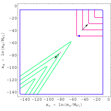
Figure 3: The possible range of $m_{i}$, $i=u,d$, is from $Y_{i}f_{\pi}^{3}/M_{P\ell}^{2}$ to $Y_{i}M_{P\ell}$. The blue dot shows the observed values. The contours are of probability density in the landscape, red (green) green for the $\mu^{2}<0$ ($>0$) region. Neighboring contours differ by $e^{20}$ in probability density, increasing in the direction of the arrows.

In that figure are also plotted the contours of equal probability density in the landscape (i.e. equal amount of fine-tuning of parameters), which will be derived in section 3 under the assumption that the parameters of $M_{ij}^{2}$ have a flat probability distribution in the landscape in the interval $[-M_{*}^{2},+M_{*}^{2}]$. The red curves are contours of equal probability density in the $\mu^{2}<0$ region, and the green curves are contours of equal probability density in the $\mu^{2}>0$ region. Neighboring contours differ in probability density by a factor of $e^{20}$, with the direction of increasing probability density indicated by the arrows.

The position of the“anthropically allowed” region in Fig. 3 in which our domain is located is indicated by the blue dot. In fact, the viable region is so small that it is smaller than the blue dot in Fig. 3. Fig. 4 is a blow-up of that region of parameter space.

Since we are assuming that the Yukawa couplings of the quarks and leptons do not vary among domains, and that both the down-type quarks and charged leptons get mass from the same Higgs doublet $H_{d}$, the electron mass is given by $m_{e}=rm_{d}$, where $r$ is a fixed ratio (up to logarithmic dependence on $v_{u}$ and $v_{d}$ through the running of parameters). We take $m_{u0}=4$ MeV and $m_{d0}=7$ MeV, where the subscript zero refers to the observed values of these parameters, i.e. their values in our domain of the universe. Thus $r=0.07$.

2.1 The case of $\mu^{2}<0$

First, we will discuss the case of negative $\mu^{2}$. If $\mu^{2}$ is negative and smaller in absolute value than in our domain, that involves more fine-tuning and is thus a less probable region of parameter space. Our interest is therefore primarily in $\mu^{2}$ negative and greater than (in absolute value) or comparable to its value in our domain. That corresponds to values of $m_{u}$ and $m_{d}$ greater than or comparable to their observed values.

If $m_{d}$ is sufficiently large, then all $d$ quarks will beta decay into $u$ quarks even inside hadrons, so that the only stable hadron will be $\Delta^{++}$ ($uuu$). “Sufficiently large” in this case means large enough to overcome the extra energy required to put three quarks of the same flavor in a totally antisymmetric state, which energy we call $E_{\Delta N}$. For $v_{u}$ and $v_{d}$ near the observed weak scale $v_{0}$, $E_{\Delta N}\sim 300$ MeV. (However, there is a weak dependence of $E_{\Delta N}$ on $v_{u}$ and $v_{d}$ through the renormalization-group running of $\alpha_{s}$, due to quark thresholds.) The condition for all $d$ quarks to beta decay is $m_{d}\geq m_{u}+m_{e}+E_{\Delta N}$, or $(1-r)m_{d}\geq m_{u}+E_{\Delta N}$. This is the region above the upper blue curve in Fig. 4, which is a log-log plot. For $m_{u}$ and $m_{d}$ masses very large compared to the QCD scale, this curve asymptotically approaches the straight line $(1-r)m_{d}=m_{u}$, which is a line of slope 1 in Fig. 4.

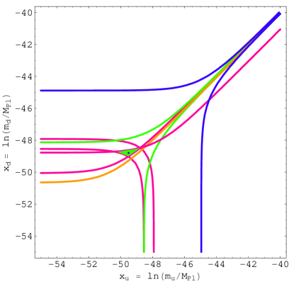
Figure 4: A blowup of the region near our domain in Fig. 3. The curves are anthropic bounds on $m_{u}$ and $m_{d}$ discussed in the text. The green shaded region is potentially viable. The dot is our domain.

For $m_{u}$ and $m_{d}$ small compared to the QCD scale, the curve asymptotically approaches the horizontal line $m_{d}=E_{\Delta N}/(1-r)$.

In the region where all the $d$ quarks decay, not only will the $\Delta^{++}$ be the only stable hadron, it will surely also be the only stable nucleus. (In this regime, $m_{d}$ is large compared to the QCD scale, so that the pions are not pseudo-goldstone particles and the range of the nuclear potential is shorter than in nuclei of our own domain. Moreover, there is a strong Coulomb repulsion between two $\Delta^{++}$.) These $\Delta^{++}$ will clothe themselves with a pair of electrons, and act chemically like helium. With the only element being helium-like, it is extremely implausible that life based on chemistry could exist.

On the other hand, if $m_{u}$ is sufficiently large compared to $m_{d}$, then all the $u$ quarks will decay to $d$, and one will have a domain in which the only stable hadron and nucleus will be a $\Delta^{-}$ ($ddd$). These will clothe themselves with positrons (which will presumably be more numerous than electrons in such a domain, due to the beta decay of all the $u$ quarks), and thus act chemically like hydrogen. An all-$\Delta^{-}$ universe is also extremely unlikely to give rise to chemistry-based life. The all-$\Delta^{-}$ universe corresponds to $m_{u}\geq m_{d}(1+r)+E_{\Delta N}$, which is the region below the lower blue curve in Fig 4. (For large quark masses this curve it is asymptotic to the line $(1+r)m_{d}=m_{u}$, which is a line of slope 1 in Fig. 4.)

Thus we can rule out almost all of the three quadrants in Fig. 4 where either $m_{u}$ or $m_{d}$ is large compared to its observed value. There is a thin ribbon between the two blue curves where both $m_{u}$ and $m_{d}$ are large compared to the QCD scale and $(1-r)m_{d}\leq m_{u}\leq(1+r)m_{d}$, where neither $d\rightarrow u+e^{-}+\overline{\nu}_{e}$ nor $u\rightarrow d+e^{+}+\nu_{e}$ can happen. However, this region is unlikely to be viable, since $A=2$ nuclei are not bound there, as shall be seen.

More of the parameter space is ruled out as viable if we take into account the conditions that both neutrons and protons should be stable inside nuclei. If $(A,Z)$ denotes a nucleus of mass $A$ and atomic number $Z$, then the process $(A,Z)\rightarrow(A-1,Z)+p+e^{-}+\overline{\nu}_{e}$ is energetically allowed if $m_{d}-m_{u}-m_{e}-\Delta m_{em}>B$, where $B$ is the binding energy of the proton in the nucleus, and $\Delta m_{em}$ is the electromagnetic contribution to the proton-neutron mass difference. Following [1], we take $\Delta m_{em}=1.7$ MeV, and we take 10 MeV as a typical value of $B$. (Of course, for very large values of $v_{u}$ and $v_{d}$, the values of $\Delta m_{em}$ and $B$ would be somewhat different. However, in that limit $\Delta m_{em}$ and $B$ are are negligible compared to $m_{u}$ and $m_{d}$ anyway, so the shape of the curves is little affected.) This gives the condition $(1-r)m_{d}\geq m_{u}+11.7$ MeV. If this is satisfied, all neutrons beta decay, even inside nuclei. Since stable nuclei having $A>1$ cannot be made up only of protons [1], the only stable nucleus in such domains and therefore the only chemical element would be ¹H. It is unlikely that chemical life can exist in an such “all hydrogen” domains. Thus viability requires that one has $(1-r)m_{d}\leq m_{u}+11.7$ MeV, which rules out the region above the upper green curve in Fig. 4. Another constraint comes from the requirement that protons should be stable in nuclei. If $m_{u}-m_{d}-m_{e}+\Delta m_{em}>B$, then protons even in nuclei would be able to decay through the process $(A,Z)\rightarrow(A-1,Z-1)+n+e^{+}+\nu_{e}$. Viability thus requires $m_{u}\leq(1+r)m_{d}+8.3$ MeV, which rules out the region below the lower green curve in Fig. 4.

A stronger bound comes from the requirement that isolated protons are stable against $p\rightarrow n+e^{+}+\nu_{e}$. If they were not, there would be no ¹H in such domains. Since almost all organic molecules (with a few exceptions, such as CO₂) contain hydrogen, a no-hydrogen domain would presumably have dim prospects for life based on chemistry. This rules out the region below the curve $m_{d}(1+r)=m_{u}+\Delta m_{em}$, shown as the orange curve in Fig. 4. A slightly stronger bound comes from the condition that the proton in the nucleus of hydrogen not convert to a neutron by electron capture $p+e^{-}\rightarrow n+\nu_{e}$, which rules out the region below the curve $m_{d}(1-r)=m_{u}+\Delta m_{em}$, shown as the lower red, concave-up curve in Fig. 4.

If the reaction $p+p\rightarrow D+e^{+}+\nu_{e}$ in the sun is to be exothermic one must have $m_{d}(1+r)\leq m_{u}+B_{D}+\Delta m_{em}$, where $B_{D}=2.2$ MeV is the binding energy of the deuteron. A very similar condition comes from requiring that the deuteron be stable against the weak decay $D\rightarrow p+p+e^{-}+\overline{\nu}_{e}$, namely $m_{d}(1-r)\leq m_{u}+B_{D}+\Delta m_{em}$. In [1] the binding energy of the deuteron was parameterized by

$$B_{D}=2.2-a\left(\frac{m_{u}+m_{d}}{m_{u0}+m_{d0}}-1\right),$$ (3)

where energies are in MeV and the parameter $a$ is very sensitive to the model of the internucleon potential. Using two different models, [1] obtained $a=5.5$ MeV and $a=1.3$ MeV. Using Eq. (3), the condition for the deuteron to be stable against weak decay becomes $(0.93-a/11)m_{d}-(1-a/11)m_{u}\leq(3.9+a)$. For $a=5.5$ MeV, this rules out the region above the upper, red, concave-up curve in Fig. 4. As noted in [1], it may be possible for the hydrogen burning to occur in stars and for nucleosynthesis to proceed even if the deuteron is unstable to weak decay, if its lifetime is sufficiently long. Thus, a more clear-cut constraint comes from the condition that the deuteron be stable against the (much faster) strong decay $D\rightarrow p+n$. The condition for this is simply that $B_{D}$ be positive. Using $a=5.5$ MeV, this gives $m_{u}+m_{d}\leq 15.4$ MeV, which rules out the region above the upper, red, concave-down curve in Fig. 4.

If the quark masses are too small, then the pion mass becomes small, and the nuclear force becomes sufficiently long-range to bind the “diproton”, i.e. the ²He nucleus, as pointed out by Dyson long ago [9]. This would allow hydrogen to burn in stars by the reaction $p+p\rightarrow^{2}$He, which is very fast as it does not involve the weak interactions. Hydrogen-burning stars would have lifetimes orders of magnitude shorter than the billions of years presumably required for complex organisms to evolve. In [1, 8] it was estimated that if $m_{u}+m_{d}<0.75(m_{u0}+m_{d0})=8.25$ MeV, the diproton is bound. This rules out the region below the lower, red, concave-down curve in Fig. 4.

Altogether, then, we see that the viable region is squeezed down to the remarkably small shaded green area bounded by the four red curves in Fig. 4. The actual value of $(m_{u},m_{d})$ observed in our domain is right in the middle of it, as shown in Fig. 4. (For perspective, recall that this shaded green region is smaller than the dot in Fig. 3, which shows the whole parameter space.)

2.2 Exotic domains with light $c$ quarks

Exotic possibilities open up if either $m_{c}$ and $m_{s}$ is small. First we shall consider the situation where $v_{u}$ is so small that $m_{c}$ becomes comparable to or smaller than $m_{d}$. (Of course, since the Yukawa coupling ratios are fixed, $m_{u}$ becomes about two orders of magnitude less than $m_{d}$.) We shall call these “light-$c$-quark domains”. In such domains the light quarks are $d$, $u$ and $c$, and there is a baryon octet made up of valence quarks of these three flavors. This octet, shown in Table I, contains baryons of charge 0, +1, and +2, but none with negative charges. Therefore these domains are similar to ours in the following respects: (1) All nuclei have $Z>0$. (2) If a nucleus has large $A$, then its charge $Z$ is also large, since Fermi energy tends to equalize the number of baryons of different species. (3) For large $Z$ nuclei, Coulomb energy becomes important and gives an upper bound to the size of stable nuclei.

$$\begin{array}[]{ccccc}&{\bf\Xi^{+}_{cc}}&&{\bf\Sigma^{0}_{c}}&\\ &(ccd)&&(cdd)&\\ &&&&\\ {\bf\Xi^{++}_{cc}}&&{\bf\Sigma^{+}_{c}},{\Lambda^{+}_{c}}&&{\bf n}\\ (ccu)&&(cud)&&(udd)\\ &&&&\\ &{\bf\Sigma^{++}_{c}}&&{\bf p}&\\ &(cuu)&&(uud)&\end{array}$$

Table I

In the light-$c$-quark part of parameter space one can distinguish three regions, which are shown in Fig. 5: (A) For large enough $m_{c}$, the lightest baryons in the octet are those without valence $c$ quarks, namely $p$ and $n$. For nuclei composed of $p$ and $n$ the analysis of the previous subsection applies. Consequently, case (A) does not give any anthropically allowed regions of parameter space except those we have already discussed. (B) For small enough $m_{c}$, the lightest baryons in the octet are those with only valence $c$ and $u$ quarks, namely $\Sigma^{++}_{c}$ and $\Xi^{++}_{cc}$ (i.e. $uuc$ and $ucc$, respectively). As we shall see, domains of this sort seem unlikely to be viable. (C) For intermediate values of $m_{c}$, the lightest baryons in the octet are $p$ and $\Sigma^{++}_{c}$. Some domains of this sort may be viable.

The sufficient condition for case (A) is that $m_{n}<m_{\Sigma^{++}_{c}}$, which gives $2m_{d}<m_{c}+m_{u}+\Delta m^{\prime}_{em}$, where the last term is the electromagnetic contribution to the splitting of $\Sigma^{++}_{c}$ and $n$. We may neglect $m_{u}$ in this expression, since it is less than a percent of $m_{c}$. We take $\Delta m^{\prime}_{em}=4\Delta m_{em}=6.8$ MeV. (Note that the observed splitting between $\Sigma^{++}_{c}$ and $\Sigma^{0}_{c}$ is 0.3 MeV, so that if the quark mass contribution is $2(m_{u}-m_{d})=-6$ MeV, it implies an electromagnetic contribution of 6.3 MeV. Of course, the wavefunctions for the charmed baryons would be different in the light-$c$-quark domains.) The condition is then $m_{c}>2m_{d}-6.8$ MeV. This is the region to the right of the lower red curve in Fig. 5.

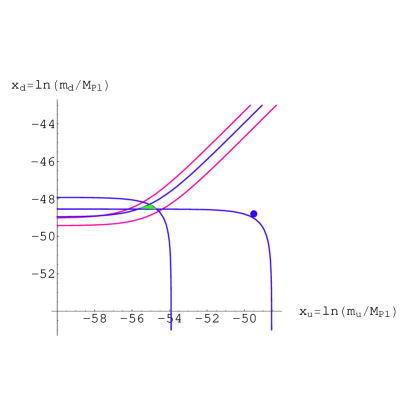
Figure 5: The “light-$c$-quark” region of parameter space. The green shaded region may be viable. The dot is our domain.

In this region, the analysis we gave in section 2 applies, and one expects that only anthropically allowed region is that shown in Fig. 4, which includes our domain (indicated by the blue dot in Fig. 5).

The condition for case (B) is that $m_{\Xi^{++}_{cc}}<m_{p}$, which gives $2m_{c}+3\Delta m_{em}<m_{d}+m_{u}$, or approximately $m_{c}<m_{d}/2-2.5$ MeV. This is the region to the left of the upper red curve in Fig. 5. This region seems unlikely to be viable since all stable nuclei would have $Z\geq 2$. (It is easily seen that an isolated $p$ will beta decay to $\Sigma^{++}_{c}$, as will a $p$ bound with neutral baryons.) Consequently, there would be no chemical analogue of hydrogen.

The most interesting case is (C), which lies in between the two red curves in Fig. 5. Here the lightest two baryons are $p$ and $\Sigma^{++}_{c}$. In such a domain, the only $Z=1$ nucleus consists of a single proton, i.e. ¹H. In order for hydrogen to be stable, it is required that the decay $p\rightarrow\Sigma_{c}^{++}+e^{-}+\overline{\nu}_{e}$ be energetically forbidden, which gives the condition $m_{c}>m_{d}(1-r)-3\Delta m_{em}$. This rules out the region above the blue, concave-up curve in Fig. 5. A second condition is that diprotons not be bound, as otherwise hydrogen-burning stars would burn too fast, as noted above. This gives the bound that $m_{d}+m_{u}>8.25$ MeV, as given previously. This rules out the region below the nearly horizontal blue line that barely misses our domain in Fig. 5.

A third condition is that the $A=2$ nucleus composed of a $p$ and a $\Sigma_{c}^{++}$ be bound. Let us call this analogue of the deuteron $\tilde{D}$. The potential between the $p$ and the $\Sigma_{c}^{++}$ at large distances is given by one-$D$-meson exchange rather than one-pion-exchange, and is thus controlled by $m_{c}+m_{d}$ rather than by $m_{u}+m_{d}$. Using Eq. (3), the binding energy of $\tilde{D}$ can be written $B_{\tilde{D}}=2.2-E_{c}-a[(m_{c}+m_{d})/(m_{u0}+m_{d0})-1]$, where $E_{c}$ is the Coulomb interaction energy of the baryons in the $\tilde{D}$. The condition that $\tilde{D}$ be bound is then $m_{c}+m_{d}<11[(2.2-E_{c})/a+1)$, where energies are in MeV. If $a=5.5$ MeV and $E_{c}=2$ MeV, this rules out the region above the blue, concave-down curve in Fig. 5.

The combination of the three constraints leaves only the very small triangular region shaded green in Fig. 5. In fact, since the three curves depend on quantities that are not well known, such as $a$, $E_{c}$, $m_{u0}$, $m_{d0}$, it is not really clear that any area is actually enclosed by them. Furthermore, even if there is, it does not necessarily mean that this area is an anthropically allowed region of parameter space. It only means that three of the more obvious disasters for viability do not happen. One other potential problem for viability is that nucleosynthesis may be inhibited in such domains because of large Coulomb barriers, due to the fact that nuclei are composed of charge-1 and charge-2 baryons. A much more serious potential problem for viability is that $G_{F}$ is about four orders of magnitude larger in this region of parameter space than it is in our domain. This would make the “$pp$ reaction” $p+p\rightarrow\tilde{D}+e^{-}+\overline{\nu}_{e}$ proceed in hydrogen-burning stars very much faster than the ordinary $pp$ reaction does in our domain. That would presumably be disastrous for the same reason that the diproton being bound would be.

As we shall see in section 3, where we discuss probability distributions in parameter space under some simple and reasonable assumptions, these potentially viable light-$c$-quark domains occur less commonly in the universe than domains like our own. Therefore, unless a typical domain of this sort is more viable than ours, the existence of such domains should not affect the anthropic explanation of the observed values of $m_{u}$ and $m_{d}$ that we are exploring here.

2.3 Exotic domains with light $s$ quarks

We now consider the situation where $v_{d}$ is so small that the mass of the $s$ quark is comparable to or smaller than $m_{u}$. (Of course, then $m_{d}\ll m_{u}$, since we are assuming that the ratios of Yukawa coupling are fixed.) We will call these “light-$s$-quark domains”. In such domains, the lightest three quarks are $d$, $s$, and $u$, as in our domain, but the corresponding flavor $SU(3)$ is a very good symmetry, since $m_{s}$ is small. Consequently, there is the familiar baryon octet, shown in Table II, but it is more nearly degenerate than in our domain.

$$\begin{array}[]{ccccc}&{\bf\Xi^{0}}&&{\bf\Sigma^{+}}&\\ &(uss)&&(uus)&\\ &&&&\\ {\bf\Xi^{-}}&&{\bf\Sigma^{0}},{\Lambda^{0}}&&{\bf p}\\ (dss)&&(uds)&&(uud)\\ &&&&\\ &{\bf\Sigma^{-}}&&{\bf n}&\\ &(dds)&&(udd)&\end{array}$$

Table II

There are three cases to consider for light-$s$-quark domains (just as there were for light-$c$-quark domains). These are shown in Fig. 6. (A) For large enough $m_{s}$, the lightest two baryons are the two non-strange baryons $p$ and $n$, as in our domain. The condition for this is that $m_{\Sigma^{-}}>m_{p}$, which gives $m_{s}+m_{d}>2m_{u}$. This is the region above the upper red curve in Fig. 6. (B) For small enough $m_{s}$, $u$ is heavier than both $s$ and $d$ and the lightest two baryons are $\Sigma^{-}$ and $\Xi^{-}$, which have no valence $u$ quarks. The condition for case (B) is that $m_{\Xi^{-}}<m_{n}$, which gives $m_{u}+m_{d}>2m_{s}+\Delta m_{em}$. This is the region below the lower red curve in Fig. 6. (C) For intermediate $m_{s}$, the lightest two baryons would be $n$ and $\Sigma^{-}$. This is the region between the two red curves in Fig. 6.

For case (A), where the lightest baryons are $p$ and $n$, as in our domain, the analysis of viability we presented earlier applies, and so the only anthropically allowed region is that shown in Fig. 4, which includes our domain (indicated by the blue dot in Fig. 6).

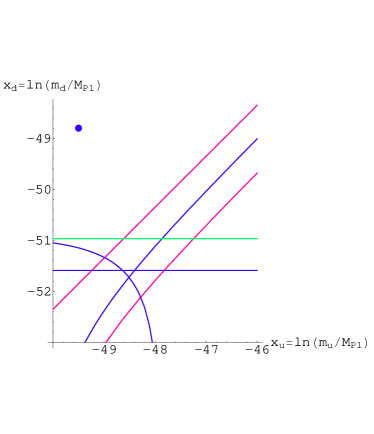
Figure 6: The “light-$s$-quark region of parameter space. Some of the region below the green line and to the right of the rightmost red curve may be viable. The dot is our domain.

Case (C) is interesting because it might lead to domains in which the $\Sigma^{-}$ plays the role that the proton plays in our domain. For example, a “hydrogen atom” in such a domain would consist of a $\Sigma^{-}$ and an $e^{+}$. (One would expect antileptons to predominate in such domains because of charge neutrality.) There are at least three constraints that $m_{u}$ and $m_{s}$ must satisfy in case (C).

First, the $\Sigma^{-}$ in the nucleus of the “hydrogen” atom must be stable against beta decay into $n+e^{-}+\overline{\nu}_{e}$. This gives the constraint $m_{u}>(1-0.05r)m_{s}+\Delta m_{em}$. This rules out the region to the left of the blue curve that is concave to the right in Fig. 6.

The second constraint is that the $n$ and $\Sigma^{-}$ must be able to bind to make the analogue of the deuteron. The long-distance part of the potential between these nucleons is controlled by the mass of the kaon, and thus by $m_{u}+m_{s}$. Thus the condition for the $n$ and $\Sigma^{-}$ to bind is $m_{u}+m_{s}<15.4$ MeV, if $a=5.5$ MeV. This rules out the region above the blue curve that is concave to the left in Fig. 6. The third constraint is that the di-$\Sigma^{-}$ not be bound (the analogue of the diproton not being bound in our domain). This gives $m_{s}+m_{d}>8.25$ MeV, which rules out the region above the nearly horizontal blue line in Fig. 6. Altogether, there is no allowed region left for case (C). However, this depends on the value of $a$, and other parameters that are not precisely known. If $a$ is less than about 3 MeV, there may be a small region that satisfies the three constraints. Of course, even if there were, that hardly proves that such a region is anthropically allowed; it merely means that some obvious disasters for viability are avoided.

We turn now to case (B). In this case the lightest baryons are $\Sigma^{-}$ and $\Xi^{-}$, and $\Sigma^{-}$ is the lighter of the two. The only obvious constraint is that the analogue of deuterium (i.e. a bound state of $\Sigma^{-}$ and $\Xi^{-}$) be allowed to form. For $a=5.5$ MeV, this gives the constraint $m_{s}+m_{d}=1.05m_{s}<15.4$ MeV. This rules out the region above the horizontal green curve in Fig. 6.

There may be some anthropic upper bound on $m_{u}$, coming from the fact that very large $m_{u}$ corresponds to very small $G_{F}$; however, that is not clear. If $v_{u}$ is superlarge and therefore $G_{F}\sim v^{-2}$ is supersmall, rather strange situations are possible. Even though $G_{F}$ is supersmall, the decay rates of $u$, $c$, and $t$ quarks, being of order $G_{F}^{2}m_{u,c,t}^{5}\sim v_{u}$ will be very fast, and the only quarks around will be $d$, $s$, and $b$. The amplitudes for transitions of $d$, $s$, and $b$ into each other will be suppressed by a factor of $v_{u}^{-2}$ and therefore, in effect, there will be separate conservation of $d$-number, $s$-number, and $b$-number. (Sphaleron processes will, of course also be highly suppressed.) The story is similar for the leptons; there will be separate conservation of $L_{e}$, $L_{\mu}$, and $L_{\tau}$.

In this case, much depends on the details of primordial lepto/baryogenesis. It is possible that lepto/baryogenesis leads to asymmetries for $d$, $s$, and $b$ quarks that differ in sign. For example, there could be an excess of $d$ over $\overline{d}$, but of $\overline{s}$ over $s$ and $\overline{b}$ over $b$. In that case, “ordinary” hadronic matter would be made up of $d$, $\overline{s}$, and $\overline{b}$. In particular, there would be stable $K^{0}$, $B^{0}$ mesons, $\Sigma^{-}$ baryons, and positively charged antibaryons consisting of valence $\overline{s}$ and $\overline{b}$. These could capture leptons of positive or negative charge (as the case may be) and make atoms. In the same way, there could be asymmetries of different sign for different flavors of lepton. For instance, there could be an excess of $e^{-}$ and $\mu^{-}$ but of $\tau^{+}$. Thus there could be atoms consisting of an $e^{-}$ orbiting a $\tau^{+}$. Clearly, all sorts of rich and strange possibilities for chemistry might exist. And if the chemistry is rich, then it is plausible that life might be possible. However, in order to have any nuclei with $Z>1$, one still needs two baryons to be able to bind. There is still, therefore, an anthropic upper bound on $m_{d}+m_{s}$ for case (B), as discussed above. As is clear from the shape of the probability contours shown in Fig. 3 and derived in section 3, this will put an upper bound on the probability density of viable small-$s$-quark domains.

In sum, there are regions of parameter space with $m_{s}$ of order a few MeV, and in particular case (B), where we have found no very obvious convincing argument against viability. There may also be a small anthropically allowed region where $m_{c}$ is of order a few MeV. As we will see in section 3, for certain plausible assumptions about the probability distribution in the $\ln m_{u}-\ln m_{d}$ plane, the possibility of such exotic viable light-$s$-quark or light-$c$-quark domains would not affect the anthropic explanation of the observed values of $m_{u}$ and $m_{d}$ being explored in this paper.

2.4 The case of $\mu^{2}>0$

In domains where $\mu^{2}>0$ the vacuum expectation value of $H_{<}$ is of order $f_{\pi}^{3}/\mu^{2}$ and therefore extremely small compared to its value in our domain. This means, of course, that in these domains the quark and lepton masses are correspondingly small. (For example, if $\mu^{2}\cong+(100{\rm GeV})^{2}$ and $\tan\beta$ is the same as in our domain, then the electron mass is only about $5\times 10^{-4}$ eV.) This has important consequences for life based on chemistry. The reason is that the energies of typical atomic and molecular transitions are of order, or smaller than, $\alpha^{2}m_{e}$, and therefore so are the temperatures needed for biological processes to occur. (That is why in our domain the temperature needed for life is about 300 K $\cong 10^{-3}\alpha^{2}m_{e0}$.) It follows that before life based on chemistry can appear the universe has to have cooled down to a temperature much smaller than $\alpha^{2}m_{e}$.

Because $m_{e}$ is so small in positive-$\mu^{2}$ domains, it was argued in [1] that by the time the universe cools sufficiently for chemistry-based life to exist in those domains various disasters might already have occurred, such as all baryons having decayed away or all stars having burned out. Those arguments depended crucially on the assumption that universe expands as a power of $t$. However, it now appears that after dark energy comes to dominate the universe will expand exponentially in $t$. Once the expansion becomes exponential, it does not take long for the universe to reach extremely small temperatures. For example, consider a domain where $m_{e}=5\times 10^{-4}$ eV. If there were no dark energy, it would take such a domain about $10^{20}$ years to reach temperatures of order $10^{-3}\alpha^{2}m_{e}$. On the other hand, if there were the observed amount of dark energy, it would take only about $10^{11}$ years. The difference is even more dramatic if $\mu^{2}$ is larger. In a typical domain where $\mu^{2}\cong(10^{10}{\rm GeV})^{2}$, it would take about $10^{44}$ years to reach biochemical temperatures if there were no dark energy, but only about $10^{13}$ years if there is the amount of dark energy we observe.

The existence of dark energy means that the specific astrophysical and cosmological anthropic arguments used for the positive-$\mu^{2}$ case in [1] are not valid. However, there are other anthropic arguments based on astrophysical and cosmological considerations that become possible precisely because of the existence of dark energy, as we will now see. For the rest of the paper we will assume that the dark energy has $w=-1$ and will refer to it as “the cosmological constant”. Our arguments should not be qualitatively affected if $w$ is not exactly $-1$.

It seems reasonable to suppose that life requires the existence of planets upon which to evolve. A planet is supported against gravitational collapse by the electrons, and has therefore a typical density that goes as $\rho_{planet}\sim Am_{p}(\alpha m_{e}/2)^{3}$, where $A$ is the average number of baryons per nucleus. A planet will be ripped apart by the inflation caused the cosmological constant, unless

$$\rho_{\Lambda}<\rho_{planet}\sim A\alpha^{3}m_{e}^{3}m_{p}.$$ (4)

If $\rho_{\Lambda}$ is truly a constant of nature, so that it the same in every domain, then its measured value of about $10^{-123}M_{P\ell}^{4}$ means that planets can exist only if $m_{e}>6\times 10^{-5}$ eV. For $\tan\beta$ having the same value as in our domain, this means that $\mu^{2}$ has to be less than about (300 GeV)². This is significantly stronger than the bound given in Eq. (6) of [1] (a bound that came from not having baryons decay away before the universe cooled to temperatures where chemical life could exist).

However, it is more interesting to suppose that $\rho_{\Lambda}$, as well as the Higgs mass parameters, varies among domains. Indeed, this comports with the idea that all the dimensionful parameters of the Lagrangian are determined anthropically. In that case one has to consider simultaneously the probability distributions of $\mu^{2}$, $\tan\beta$ and $\rho_{\Lambda}$. This will be done in section 4. It will be seen that the viability of a significant part of the positive $\mu^{2}$ parameter space is left unaffected by the “planet argument”. However, most of that part of parameter space can be anthropically ruled out by a second argument, which is based on structure formation.

That second argument assumes that structure cannot begin to form until recombination occurs. If by the time of recombination the density of the universe is already dominated by the cosmological constant, then structure will never form. The recombination temperature $T_{rec}$ is about $0.05\alpha^{2}m_{e}$, so the constraint is that structure cannot form unless

$$\rho_{\Lambda}<\rho_{B}(t_{rec})\sim m_{p}\eta_{B}T_{rec}^{3}\sim 10^{-14}\alpha^{6}m_{e}^{3}m_{p}.$$ (5)

This appears to be a much more stringent constraint than the one in Eq. (4). However, it is not clear that it can be used for $m_{e}$ smaller than about 20 eV. The point is that, if $m_{e}<20$ eV, then when matter begins to dominate over radiation (at $T\sim 1$ eV) the electrons will still be almost relativistic, and the thermal number density of electrons and positrons will be larger than that of the baryons by a factor of about $10^{10}e^{-m_{e}/T}$. There will then be of order $10^{10}$ electrons and positrons for each baryon. The charges of the baryons will be Debye screened, and it would seem that baryons can already begin to condense at that point, since $\delta\rho_{B}/\rho_{B}$ would not have a significant effect on the density of the leptons and photons. We will therefore only use Eq. (5) when $m_{e}>20$ eV. The anthropic bounds coming from Eqs. (4) and (5) will be analyzed in section 4.

3 Probability distributions in the $\ln m_{u}-\ln m_{d}$ plane

Since anthropic explanations of relations among parameters are based on probabilities, one must be able to make reasonable hypotheses about probability distributions within the parameter space or “landscape”. The parameters that we are assuming to vary among domains of the universe are those in the Higgs mass-squared matrix $M^{2}_{ij}$. This matrix acts in the space of $\left(\begin{array}[]{c}H_{u}\\ \tilde{H}_{d}\end{array}\right)$. It is convenient to parameterize this matrix as follows

$$M^{2}=\left(\begin{array}[]{cc}a_{0}+a_{3}&a_{1}-ia_{2}\\ a_{1}+ia_{2}&a_{0}-a_{3}\end{array}\right).$$ (6)

First, we will assume that the four real parameters $a_{\alpha}$ (which have dimensions of mass squared) are “naturally” superlarge (either $O(M_{GUT}^{2})$ or $O(M_{P\ell}^{2})$) and of the same order. Call their natural scale $M_{*}^{2}$. The simplest assumption is that the four $a_{\alpha}$ are independent and that each has a flat probability distribution in the interval $[-M_{*}^{2},+M_{*}^{2}]$. (However, symmetry may somewhat suppress the off-diagonal elements of $M_{ij}^{2}$. We will discuss the effects of this later.) We will take $a_{0}$ to be positive. (If it is negative and very large the weak interactions are broken at very large scales, whereas if it is negative and small then breaking the weak interactions at small scales would require that $a_{3}$ also be small, which is an extra fine tuning.) It is convenient to think of the parameters $a_{1}$, $a_{2}$, and $a_{3}$ as forming the components of a vector $\vec{a}$ in a three-dimensional space. As these three parameters have been assumed all to have flat probability distributions in the interval $[-M_{*}^{2},+M_{*}^{2}]$, the probability distribution is rotationally invariant in the space of $\vec{a}$.

We shall denote the larger eigenvalue of $M^{2}_{ij}$ by $M^{2}_{>}$ and the smaller eigenvalue by $\mu^{2}$. (By our assumption about $a_{0}$, $M_{>}^{2}$ is positive.) Since $M^{2}_{>}$ is generally much larger than $\mu^{2}$, the heavier Higgs doublet decouples; so the parameter $\mu^{2}$ is in effect just the $\mu^{2}$ of the Standard Model and controls the breaking of the weak interactions. Because the cases of anthropic interest are those where $|\mu^{2}|\ll M_{>}^{2}$, we may write

$$\mu^{2}\cong\frac{\det M^{2}}{{\rm tr}M^{2}}=\frac{a_{0}^{2}-\vec{a}^{2}}{2a_{0}},$$ (7)

$$\tan 2\beta=\frac{2|M^{2}_{ud}|}{M^{2}_{uu}-M^{2}_{dd}}=\frac{\sqrt{a_{1}^{2}+a_{2}^{2}}}{a_{3}}=\tan\theta_{a},$$ (8)

where $\beta$ is the angle between the mass basis of the Higgs doublets $(H_{>},H_{<})$ and the original flavor basis $(H_{u},\tilde{H}_{d})$ (i.e. $H_{<}=e^{i\alpha}\sin\beta H_{u}+\cos\beta\tilde{H}_{d}$ and $\tan\beta=\left|\frac{v_{u}}{v_{d}}\right|$), and $\theta_{a}$ is the angle between $\vec{a}$ and the $a_{3}$ axis. There are two cases to consider, $\mu^{2}<0$ and $\mu^{2}>0$.

3.1 Probability distribution in the case of $\mu^{2}<0$

In the case of negative $\mu^{2}$, the vacuum expectation value that breaks the weak interactions is $v=\sqrt{|\mu^{2}|/\lambda}=(2\lambda)^{-1/2}$ $\left|(a_{0}^{2}-a^{2})/a_{0}\right|^{1/2}$, where $a$ is the magnitude of $\vec{a}$, and $\lambda$ is the quartic self-coupling of the lighter Higgs doublet. Then we may write $m_{u}=Y_{u}v_{u}=Y_{u}v\sin\beta\cong(Y_{u}/\sqrt{2\lambda})$ $\sin\frac{\theta_{a}}{2}\sqrt{(a_{0}^{2}-a^{2})/a_{0}}$, and similarly $m_{d}=Y_{d}v_{d}=Y_{d}v\cos\beta\cong(Y_{d}/\sqrt{2\lambda})\cos\frac{\theta_{a}}{2}$ $\sqrt{(a_{0}^{2}-a^{2})/a_{0}}$. Defining $K=Y_{u}/\sqrt{2\lambda}$ and recalling the definition of $k$ in Eq. (2), one has

$$\begin{array}[]{cl}&m_{u}=K\sin\frac{\theta_{a}}{2}\sqrt{(a_{0}^{2}-a^{2})/a_{0}},\\ m_{d}/k\equiv&\overline{m_{d}}=K\cos\frac{\theta_{a}}{2}\sqrt{(a_{0}^{2}-a^{2})/a_{0}}.\end{array}$$ (9)

Since, by our assumptions, the probability distribution is rotationally invariant in the space of the vector $\vec{a}$, one may write the probability distribution in spherical coordinates $(a,\theta_{a},\phi_{a})$ in that space:

$$P(a_{0},a,\theta_{a},\phi_{a})\;da_{0}\;da\;d\theta_{a}\;d\phi_{a}=N\;da_{0}\;a^{2}\;da\;\sin\theta_{a}\;d\theta_{a}\;d\phi_{a},$$ (10)

where $N$ is the appropriate normalization factor. We would like to compute the probability distribution in the space of $m_{u}$ and $m_{d}$. Thus we write $P(a_{0},a,\theta_{a})da_{0}\;da\;d\theta_{a}\;d\phi_{a}=P(a_{0},m_{u},\overline{m_{d}})da_{0}\;dm_{u}\;d\overline{m_{d}}\;d\phi_{a}$, and compute the Jacobian for the transformation of coordinates:

$$J=\left|\frac{\partial(a_{0},m_{u},\overline{m_{d}})}{\partial(a_{0},a,\theta_{a})}\right|=\frac{1}{2}K^{2}(a/a_{0}).$$ (11)

This yields the result

$$P(a_{0},m_{u},\overline{m_{d}})=2N\;K^{-2}\;a_{0}\;a\;\sin\theta_{a}.$$ (12)

¿From Eq. (9), one has $a=\sqrt{a_{0}^{2}-a_{0}K^{-2}(m_{u}^{2}+\overline{m_{d}}^{2})}$ and

$$\sin\theta_{a}=\frac{2m_{u}\overline{m_{d}}}{m_{u}^{2}+\overline{m_{d}}^{2}}.$$ (13)

This yields

$$P(a_{0},m_{u},\overline{m_{d}})=4N\;K^{-2}\;a_{0}\;\sqrt{a_{0}^{2}-a_{0}K^{-2}(m_{u}^{2}+\overline{m_{d}}^{2})}\frac{m_{u}\overline{m_{d}}}{m_{u}^{2}+\overline{m_{d}}^{2}}.$$ (14)

For the regions of parameter space that are anthropically interesting (i.e. where life is likely to be possible) one has $K^{-2}m_{u}^{2},K^{-2}\overline{m_{d}}^{2}\ll a_{0}\sim M^{2}_{*}$, so that the previous equation can be written $P(a_{0},m_{u},\overline{m_{d}})=4NK^{-2}a_{0}^{2}m_{u}\overline{m_{d}}/(m_{u}^{2}+\overline{m_{d}}^{2})$. One then simply integrates over the variable $a_{0}$ to get

$$P(m_{u},\overline{m_{d}})\;dm_{u}\;d\overline{m_{d}}=N^{\prime}\frac{m_{u}\overline{m_{d}}dm_{u}d\overline{m_{d}}}{m_{u}^{2}+\overline{m_{d}}^{2}},\;\;{\rm for}\;\;\mu^{2}<0.$$ (15)

It is more interesting to express the probabilities in terms of the logarithms of the quark masses. Defining $x_{u}=\ln(m_{u}/M_{*})$, $x_{d}=\ln(m_{d}/M_{*})$, and $\overline{x_{d}}=\ln(\overline{m_{d}}/M_{*})=x_{d}-\ln k$, one has

$$P(x_{u},x_{d})\;dx_{u}\;dx_{d}=N^{\prime\prime}\frac{e^{2x_{u}+2\overline{x_{d}}}}{e^{2x_{u}}+e^{2\overline{x_{d}}}}\;dx_{u}\;d\overline{x_{d}},\;\;{\rm for}\;\;\mu^{2}<0.$$ (16)

The contours of constant probability given by this expression are plotted as the concave-up curves in Fig. 3. Note the shift represented by the fact that $P$ depends on $\overline{x_{d}}=x_{d}-\ln k$, where $k\simeq 10^{2}$. This shift means that domains where $m_{d}\cong m_{d0}$ and $k^{-1}m_{u0}<m_{u}<m_{u0}$ are just as likely to occur as domains like ours. The reason for this is simple. In our domain, one has $m_{d}\sim m_{u}$, even though $Y_{d}=kY_{u}\gg Y_{u}$. This means that $v_{u}/v_{d}=\tan\beta\simeq k\gg 1$, so that $v=\sqrt{v_{u}^{2}+v_{d}^{2}}\cong v_{u}$. Reducing $m_{u}$ from its value in our domain ($m_{u0}$) while holding $m_{d}$ fixed, means reducing $v_{u}$ while holding $v_{d}$ fixed. This has the effect of reducing $v$ and thus $\mu^{2}$, which increases the fine tuning. However, it also has the effect of making the ratio $v_{u}/v_{d}$ closer to one, which reduces the fine-tuning. (The factor of $\sin\theta_{a}=\sin 2\beta$ in $P$ prefers equal values of $v_{u}$ and $v_{d}$.) These effects cancel, so that it does not “cost probability” to move to the left in Fig. 2 from the point representing our domain down to values $m_{u}\sim k^{-1}m_{u0}$. Decreasing $m_{u}$ more than that does cost probability, however, because it means making $v$ and $\mu^{2}$ more fine-tuned without any compensating effect from $\tan\beta$, which indeed starts to move away again from 1 towards 0.

Thus, to explain why we don’t observe a value of $m_{u}$ as small as $k^{-1}m_{u0}\sim 10^{-2}m_{u0}$, one cannot argue that such domains are less common. Rather, one has to argue that they are less viable. In fact, we have presented such arguments in section 2. What makes the region of parameter space with $m_{u}\ll m_{u0}$ less viable is a combination of constraints coming from reactions in hydrogen-burning stars like the sun, as one sees from Fig. 4. If $m_{u}$ is even slightly smaller than $m_{u0}$, it either makes the $pp$ reaction $p+p\rightarrow D+e^{+}+\nu_{e}$ endothermic (since protons become lighter relative to neutrons), or it makes the diproton a bound state, allowing the reaction $p+p\rightarrow$ ²He, or it has both effects. Another effect that is probably deleterious to the chances of life is that as $v_{u}$ gets smaller $v$ gets smaller, as mentioned, and so $G_{F}$ gets larger. This would make the $pp$ reaction go much faster (since it involves the weak interaction), presumably making stars like the sun burn much faster. However, we have not calculated this effect, since the reaction $p+p\rightarrow$ ²He being allowed is an even more drastic effect.

3.2 Probability distribution in the case of $\mu^{2}>0$

If $\mu^{2}$ is positive, then the light Higgs doublet $H_{<}$ only acquires a vacuum expectation value due to quark-antiquark condensation at $f_{\pi}$, the chiral-symmetry-breaking scale of QCD. Specifically, the lighter Higgs doublet has the coupling $H_{<}(Y_{t}\sin\beta\overline{t}t+Y_{b}\cos\beta\overline{b}b)$. After QCD chiral symmetry breaking this produces a linear term in the effective potential for $H_{<}$ that is of the form $(Y_{t}\sin\beta+Y_{b}\cos\beta)f_{\pi}^{3}H_{<}$. Since we have assumed that $Y_{t}\simeq Y_{b}\simeq 1$, the coefficient $(Y_{t}\sin\beta+Y_{b}\cos\beta)$ is a slowly varying function of $\beta$ that is of order 1. We will denote this $\gamma(\beta)$.

Then instead of Eq. (9) one has

$$\begin{array}[]{cl}&m_{u}=Y_{u}\gamma(\beta)f_{\pi}^{3}\sin\frac{\theta_{a}}{2}\left((a_{0}^{2}-a^{2})/2a_{0}\right)^{-1}\\ m_{d}/k\equiv&\overline{m_{d}}=Y_{u}\gamma(\beta)f_{\pi}^{3}\cos\frac{\theta_{a}}{2}\left((a_{0}^{2}-a^{2})/2a_{0}\right)^{-1}.\end{array}$$ (17)

Thus, the Jacobian is given not by Eq. (11) but by

$$J=(Y_{u}\gamma(\beta)f_{\pi}^{3})^{2}4a_{0}a^{2}/(a_{0}^{2}-a^{2})^{3}.$$ (18)

There may be values of $\beta$ for which $\gamma(\beta)\ll 1$ due to an almost exact cancelation between the $Y_{t}$ term and the $Y_{b}$ term. However, that simply makes $m_{u}$ and $m_{d}$ small. Since smaller values of $m_{u}$ and $m_{d}$ are the the most probable ones anyway in the case of $\mu^{2}>0$, the possibility of such cancelations has virtually no effect on the probability distribution we shall derive. Thus we will get qualitatively the right behavior for $P(m_{u},m_{d})$ if we treat $\gamma$ as a constant, which we will now do for simplicity. Then following the same steps as before one ends up with

$$P(m_{u},\overline{m_{d}})\;dm_{u}\;d\overline{m_{d}}=\tilde{N}^{\prime}\frac{m_{u}\overline{m_{d}}dm_{u}d\overline{m_{d}}}{(m_{u}^{2}+\overline{m_{d}}^{2})^{5/2}},\;\;{\rm for}\;\;\mu^{2}>0.$$ (19)

and, in terms of the variables $x_{u}$ and $\overline{x_{d}}$,

$$P(x_{u},x_{d})\;dx_{u}\;dx_{d}=\tilde{N}^{\prime\prime}\frac{e^{2x_{u}+2\overline{x_{d}}}}{(e^{2x_{u}}+e^{2\overline{x_{d}}})^{5/2}}\;dx_{u}\;d\overline{x_{d}},\;\;{\rm for}\;\;\mu^{2}>0.$$ (20)

The probability contours for both positive and negative $\mu^{2}$ that we have just derived have been displayed in Fig. 3. For negative $\mu^{2}$ the probabilities increase upward and to the left (i.e. towards larger $m_{u}$ and $m_{d}$), whereas for positive $\mu^{2}$ the probabilities increase downward and to the left (i.e. toward smaller $m_{u}$ and $m_{d}$). The directions of increasing probability are shown by the arrows and the contours with equal probability to our own domain are shown by the red curves. We see from this that the potentially viable “light-$s$ quark domains” and “light-$c$-quark domains” are less common than domains like our own.

In deriving the probability distributions given in Eqs. (16) and (20), we assumed that all the elements of the Higgs mass matrix $M^{2}_{ij}$ have the same natural scale $M_{*}^{2}$. However, the “natural flavor conservation” [5] pattern of Yukawa couplings that we have assumed in Eq. (1) (whereby $H_{u}$ couples to up-type quarks and $H_{d}$ couples to down-type quarks and charged leptons) is not “technically natural” unless there is a symmetry $K$ under which $H_{u}$ and $\tilde{H}_{d}$ transform differently. The off-diagonal elements of $M^{2}_{ij}$ necessarily break this symmetry. If $K$ is a global symmetry, then one can simply regard the $d=2$ term $M_{ud}^{2}H_{u}^{{\dagger}}\tilde{H}_{d}$ as a soft breaking of $K$. In that case, the pattern of Yukawa couplings in Eq. (1) is still technically natural. It would be reasonable to assume that the natural scale of $M^{2}_{ud}$ was the same as that of $M^{2}_{uu}$ and $M^{2}_{dd}$.

On the other hand, one might imagine that $K$ is spontaneously broken. For example, suppose $M^{2}_{ud}$ arises from a $K$-invariant term $\epsilon H_{u}^{{\dagger}}\tilde{H}_{d}S^{2}$, where $S$ has a potential $V(S)=\frac{1}{4}\lambda_{S}(|S|^{2})^{2}+\mu^{2}_{S}|S|^{2}$. Then it would be consistent with our approach to say that $\mu^{2}_{S}$ scanned and had a natural scale $M^{2}_{*}$. In this scenario, there are two equally probable cases, $\mu_{S}^{2}>0$ and $\mu_{S}^{2}<0$. For $\mu^{2}_{S}<0$, the natural scale of $M_{ud}^{2}$ is $\epsilon\lambda_{S}^{-1}M_{*}^{2}$. If $\epsilon\lambda_{S}^{-1}$ is small, the probability distribution $P(x_{u},x_{d})$ is suppressed when $v_{u}$ and $v_{d}$ are comparable (more precisely, when they are within a factor of $\epsilon\lambda_{S}^{-1}$ of each other), i.e. near the line $x_{u}=\overline{x_{d}}$ in Fig. 3. This would not qualitatively affect our analysis unless $\epsilon\lambda_{S}^{-1}$ were very small (less than about $10^{-2}$), in which case the potentially viable small-$c$- quark and small-$s$-quark regions would start to have probability densities rivaling that of our domain. If $\mu_{S}^{2}>0$, then $M^{2}_{ud}=0$ and quite a different situation results. A single fine-tuning to make the weak scale small would leave either $M_{uu}^{2}$ or $M_{dd}^{2}$ of order $+M_{*}^{2}$. If $M_{uu}^{2}\sim+M^{2}_{*}$, the $u$, $c$, and $t$ quarks would have negligible masses, while the down quark masses would be set by the scale of weak interaction breaking. We have not investigated the viability of such domains.

In our discussions of probability distributions, we have not considered the renormalization group running of $\lambda$ and $\mu^{2}$ from the scale $M_{*}$ down to the scale $v$. This would affect the probability distributions by factors of order 1. However, it should not qualitatively affect our discussion.

4 Simultaneous tuning of the Higgs mass matrix and $\Lambda$

In section 2.4, two anthropic constraints on the relation between the mass of the electron and the cosmological constant were discussed. These eliminate as non-viable the great majority of the positive-$\mu^{2}$ parameter space. However, in order to express these as anthropic constraints on the Higgs mass parameters (or equivalently on $x_{u}=\ln(m_{u}/M_{*})$ and $x_{d}=\ln(m_{d}/M_{*})$) one must do an analysis that simultaneously takes into account the probability distributions of $x_{u}$, $x_{d}$ and $\rho_{\Lambda}$. That is done in this section. Both of the anthropic constraints on $\rho_{\Lambda}$ discussed in section 2.4 and given in Eqs. (4) and (5) require $\rho_{\Lambda}$ to be less than bounds that are proportional to $m_{e}^{3}$ and thus to $e^{3\overline{x_{d}}}$. If we assume that the probability distribution of $\rho_{\Lambda}$ among domains is flat in the interval $[-M_{P\ell}^{4},+M_{P\ell}^{4}]$, then the probability distribution given in Eq. (20) gets modified by a changed normalization factor and by an extra factor of $e^{3\overline{x_{d}}}$ to account for the tuning of the cosmological constant required to satisfy Eq. (4) or (5):

$$P^{\prime}(x_{u},x_{d})\;dx_{u}\;dx_{d}\propto\frac{e^{2x_{u}+2\overline{x_{d}}}}{(e^{2x_{u}}+e^{2\overline{x_{d}}})^{5/2}}\;e^{3\overline{x_{d}}}\;dx_{u}\;d\overline{x_{d}}.$$ (21)

The prime on this probability density indicates that this is a conditional probability: it is the probability density for being at $(x_{u},x_{d})$ subject to the condition that $\rho_{\Lambda}$ has been tuned to a small enough value to satisfy either Eq. (4) or Eq. (5). If the condition is that Eq. (4) be satisfied, we will call this $P^{\prime}_{planet}$, if the condition is that Eq. (5) is satisfied, we will call it $P^{\prime}_{structure}$.

The constant of proportionality in Eq. (21) depends on which condition is being enforced. To determine the constants of proportionality, it is convenient to start by finding the points in the positive-$\mu^{2}$ and negative-$\mu^{2}$ regions of the $x_{u}-x_{d}$ plane where $x_{u}=x_{d}$ and where the Higgs mass matrix $M^{2}_{ij}$ is fine-tuned to the same degree as in our domain (without any condition on $\rho_{\Lambda}$). We will call these point $S_{+}$ and $S_{-}$. (The $S$ stands for symmetric, since $x_{u}=x_{d}$ there, and the subscript tells whether it lies in the $\mu^{2}>0$ or $\mu^{2}<0$ region.) These points are shown in Fig. 7, where the point representing our domain is labeled D.

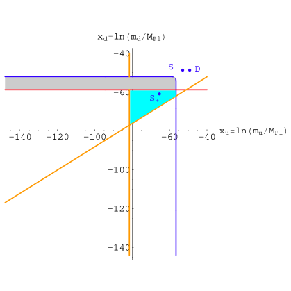
Figure 7: The $\mu^{2}>0$ region (approximately $v_{u},v_{d}<f_{\pi}$) is below and to the left of the blue curve. The arguments of section 2.4 rule out all but the shaded blue region.

Suppose that Eq. (5) implies that at $S_{+}$ the cosmological constant has to satisfy $\rho_{\Lambda}(S_{+})<p_{structure}\;\rho_{\Lambda 0}$, where $\rho_{\Lambda 0}$ is the value observed in our domain, i.e. that $\rho_{\Lambda}$ must be fine-tuned at $S_{+}$ to be less than it is in our domain by a factor smaller than $p_{structure}$. On the other hand, the Higgs mass parameters are equally fine-tuned at $S_{+}$ and in our domain, by definition of $S_{\pm}$. So the conditional probability density $P^{\prime}_{structure}$ at $S_{+}$ divided by the conditional probability density $P^{\prime}$ in our domain (where $\rho_{\Lambda}$ is tuned to $\rho_{\Lambda 0}$) is just given by $p_{structure}$. Therefore, if we define the shifted variables $\tilde{x_{u}}\equiv x_{u}-x_{u}(S_{+})$ and $\tilde{x_{d}}\equiv x_{d}-x_{d}(S_{+})$, we may write

$$\frac{P^{\prime}_{structure}(x_{u},x_{d})}{P^{\prime}(D)}<p_{structure}\;\frac{2^{5/2}e^{2\tilde{x_{u}}+5\tilde{x_{d}}}}{(e^{2\tilde{x_{u}}}+e^{2\tilde{x_{d}}})^{5/2}}.$$ (22)

Note that at $S_{+}$, where $\tilde{x_{u}}=\tilde{x_{d}}=0$, the right-hand side of the equation is just $p_{structure}$. In order to compute the coefficient $p_{structure}$, it is necessary to determine the value of $m_{e}(S_{+})$ and substitute it into Eq. (5).

At the point $D$, i.e. in our domain, one has $v_{u}=v_{u0}\simeq 174$ GeV, $v_{d}=v_{d0}\simeq 4$ GeV (if we assume $Y_{b}\simeq Y_{t}\simeq 1$), and $m_{e}=m_{e0}=Y_{e}v_{d0}\simeq Y_{e}$ (4 GeV). Since $P(S_{+})=P(S_{-})$, Eq. (16) implies that $v_{u}(S_{-})=v_{d}(S_{-})\simeq\sqrt{2}v_{d0}\simeq 4\sqrt{2}$ GeV, and therefore $v(S_{-})\simeq 8$ GeV; so that $m_{e}(S_{-})=(Y_{e}/\sqrt{2})v(S_{-})\simeq Y_{e}(4\sqrt{2}$ GeV) $\simeq\sqrt{2}m_{e0}=0.7$ MeV. On the other hand, at the point $S_{+}$, the electron mass is given by $m_{e}(S_{+})=(Y_{e}/\sqrt{2})\;(f_{\pi}^{3}/\mu^{2}(S_{+}))$. But by definition, $\mu^{2}(S_{+})=\mu^{2}(S_{-})$ and therefore $\sqrt{\mu^{2}(S_{+})/\lambda}=\sqrt{\mu^{2}(S_{-})/\lambda}=v(S_{-})\simeq 8$ GeV. Taking $\lambda\simeq 1$ we have $m_{e}(S_{+})\simeq m_{e}(S_{-})(f_{\pi}/(8{\rm GeV}))^{3}\simeq 1$ eV. Substituting this into Eq. (5), one has $\rho_{\Lambda}(S_{+})<10^{-7}\rho_{\Lambda 0}$. In other words,

$$p_{structure}\cong 10^{-7}.$$ (23)

The constraint on $\rho_{\Lambda}$ coming from Eq. (5) only applies if $m_{e}>20$ eV. The region with $m_{e}>20$ eV lies above the horizontal straight red line in Fig. 7. The region of positive $\mu^{2}$ corresponds to the area below and to the left of the blue curve in Fig. 7. (This curve arises from the fact that for very small positive $\mu^{2}$, the value of $\langle H_{<}\rangle$ is set by the competition between the quartic term $(\lambda/4)H_{<}^{4}$ and the linear term for $H_{<}$ coming from the QCD condensates of $\overline{q}q$. This gives a maximum value for $\sqrt{v_{u}^{2}+v_{d}^{2}}=\langle H_{<}\rangle\simeq f_{\pi}$ in the positive-$\mu^{2}$ region.) It is easy to see from Eqs. (22) and (23) that the entire region satisfying both $\mu^{2}>0$ and $m_{e}>20$ eV (shaded gray in Fig. 7) is much more fine-tuned than our domain, i.e. $P^{\prime}_{structure}/P^{\prime}(D)\ll 1$.

Turning now to the condition that planets be able to form (Eq. (4)), the calculation is completely parallel to the one just done. To find $p_{planet}$ one substitutes $m_{e}(S_{+})$ into Eq. (4) and divides by $\rho_{\Lambda 0}$, which gives

$$\frac{P^{\prime}_{planet}(x_{u},x_{d})}{P^{\prime}(D)}<p_{planet}\;\frac{2^{5/2}e^{2\tilde{x_{u}}+5\tilde{x_{d}}}}{(e^{2\tilde{x_{u}}}+e^{2\tilde{x_{d}}})^{5/2}}.$$ (24)

and

$$p_{planet}\simeq 3\times 10^{13}\;A,$$ (25)

where $A$ is the average atomic weight of a nucleus in the planet. It is easy to see that the region to the left of the vertical orange line or below the slanted orange line are more fine-tuned than our domain, i.e. $P^{\prime}_{planet}/P^{\prime}(D)<1$. The shape of the orange line arises from the fact that when $\tilde{x_{d}}>\tilde{x_{u}}$, the expression in Eq. (24) is approximately proportional to simply $e^{2\tilde{x_{u}}}$, whereas when $\tilde{x_{u}}>\tilde{x_{d}}$, the expression in Eq. (24) is approximately proportional to $e^{-3\tilde{x_{u}}+5\tilde{x_{d}}}$.

The two arguments given in section 2.4 have excluded (as being more fine-tuned than our domain) the whole of the positive-$\mu^{2}$ region except for the region shaded light blue in Fig. 7. However, that is not good enough. It is necessary to exclude the entire positive-$\mu^{2}$ region either as not viable or as more improbable than our domain, if the anthropic explanation of the observed values of $m_{u}$ and $m_{d}$ is to be tenable. Other arguments that were suggested in [1] hold some promise of being able to do this. For example, as noted there, it might be that the peculiarities of nuclear physics in the positive-$\mu^{2}$ region may lead to runaway nucleosynthesis. However, the situation for $\mu^{2}>0$ has many unclear aspects, and more thought must be given to it.

5 Conclusions

We have investigated the possibility that the entire mass matrix of the Higgs fields in a two-Higgs-doublet model varies among domains of a “multiverse”. This means that both the weak scale $v\equiv\sqrt{v_{u}^{2}+v_{d}^{2}}$ and $\tan\beta\equiv v_{u}/v_{d}$ vary among domains. Making plausible assumptions about probability distributions of parameters in the “landscape” and about the requirements for life, we have found that almost all of the $\ln m_{u}-\ln m_{d}$ space is either anthropically non-viable or much more fine-tuned (and therefore more rare in the multiverse) than our domain. The potentially viable regions are islands in parameter space. One of these islands is ours, and it is a very small island indeed, as seen in Figs. 3 and 4. If this is the only island of viability, there is the possibility of accounting for two otherwise not easily understood facts about the world we observe, namely that the weak scale is comparable to the strong scale, and that $m_{u}/m_{d}\sim 1$.

Whether this is in fact the only island of viability is not yet clear. There are possible islands of viability in the “light-$c$-quark” and “light-$s$-quark” regions. However, even if islands of viability do exist in those parts of parameter space they are less probable in the landscape than the island of viability in which our domain is located, according to the analysis of section 3. More significant is the possibility of an island of viability in the $\mu^{2}>0$ region of parameter space.

An interesting new twist has been given to the discussion of the positive-$\mu^{2}$ case by the discovery of dark matter/cosmological constant. This discovery ties together the anthropic analysis of the Higgs mass given in [1] and [8] and the anthropic analysis of the cosmological constant given in [10]. We have seen that some of the $\mu^{2}>0$ constraints are invalidated by the existence of dark energy, but other and equally strong constraints that depend on the existence of dark energy come into play. However, the constraints we have discussed are not by themselves enough to rule out the entire $\mu^{2}>0$ region as non-viable. This seems to be the main loophole at present in the attempt to explain $m_{u}\sim m_{d}$ and the value of the weak scale anthropically. However, it seems probable that much stronger arguments exist for the case of $\mu^{2}>0$, and that the entire positive-$\mu^{2}$ region of parameter space is non-viable.

We have assumed that only the dimensionful parameters of the Lagrangian “scan”, i.e. vary in the multiverse, and that only they are anthropically tuned. This seems like a comparatively conservative assumption, since the dimensionful parameters of our current theories are the least well understood, are the most (apparently) fine-tuned, and are the most amenable to anthropic explanation. However, obviously, other assumptions are possible. The question for us is whether there exists at least some set of plausible assumptions under which the observed relation $m_{u}\sim m_{d}$ can be anthropically explained.

References

- [1] V. Agrawal, S.M. Barr, J.F. Donoghue and D. Seckel, Phys.Rev. D57, 5480 (1998); ibid., Phys. Rev. Lett. 80, 1822 (1998).
- [2] C. Hogan, Rev. Mod. Phys. 72, 1149 (2000); S. Weinberg, hep-ph-0511037, Opening Talk at the symposium “Expectations of a Final Theory”, published in Universe or Multiuniverse?, ed. B. Carr, Cambridge University Press, 2006.
- [3] R.D. Peccei and H.R. Quinn, Phys. Rev. Lett. 38, 1440 (1977).
- [4] M.A.B. Beg and H.-S. Tsao, Phys. Rev. Lett. 41, 278 (1978); R.N. Mohapatra and G. Senjanovic, Phys. Lett. 79B, 283 (1978); H. Georgi, Had. J. 1, 155 (1978);
- [5] S.L. Glashow and S. Weinberg, Phys. Rev. D15, 1966 (1977).
- [6] S.M. Barr and I. Dorsner, Phys. Lett. B566, 125 (2003).
- [7] K.S. Babu and S.M. Barr, Phys. Lett. B381, 202 (1996).
- [8] C. Hogan, Rev. Mod. Phys. 72, 1149 (2000); Phys.Rev. D74, 123514 (2006).
- [9] F.J. Dyson, Scientific American, 225 (Sept.), 51 (1971); C. Hogan, Rev. Mod. Phys. 72, 1149 (2000)
- [10] S. Weinberg, Phys. Rev. Lett. 59, 2607 (1987).